Constraining parameters of low mass merging compact binary systems with Einstein Telescope alonePreprint: APS/123-QED
Abstract
The Einstein Telescope (ET), a future third-generation gravitational wave detector will have detection sensitivity for gravitational wave signals down to 1 Hz. This improved low-frequency sensitivity of the ET will allow the observation of low mass binaries for a longer period of time in the detection band before their merger. Because of an improved sensitivity as compared to current and advanced 2G detectors, the detection rate will also be greatly improved. Given the high detection rate of merging compact binaries with the ET, it will be a useful instrument to conduct population studies. In this paper we present an algorithm to estimate the parameters of the low mass merging compact binary systems such as localization, chirp mass, redshift, mass ratios and total mass of the source which are crucial in order to estimate the capability of the ET to study various compact binary populations. For the compact binary population distributed uniformly in comoving volume we find that with single ET, of binaries can be localized within 800 square degrees. The values of chirp mass and total mass can be constrained within error, while and can be estimated with an error of for effective SNR using single ET.
Keywords:
Gravitational waves; Methods: data analysis; Stars: neutron starsI Introduction
The second-generation gravitational wave (GW) detectors initiated GW astronomy with the first detection of merging compact objects GW150914 Abbott et al. 2016, which was the direct detection of a binary black hole (BBH). Numerous BBH detections in the next run since then have shown the existence of a population of stellar-mass black holes (BHs) undetected in previous observations which is much heavier than those detected through the observation of x-ray binaries Abbott et al. 2021; Abbott et al. 2019; Abbott et al. 2020a; Abbott et al. 2020b. The first detection of a binary neutron star (BNS) inspiral Abbott et al. 2017 with simultaneous gamma-ray burst observation and the subsequent detection of the electromagnetic counterpart provided a better understanding of the origin of short gamma-ray bursts Goldstein et al. 2017; Savchenko et al. 2017; Abbott et al. 2017a; Coulter et al. 2017; Troja et al. 2017; Hallinan et al. 2017; Abbott et al. 2017b. The observations of the associated kilonova proved that the BNS mergers source the formation of the heaviest metals through r-process nucleosynthesis. The joint detection of GWs and gamma-ray bursts proved the speed of GW and the speed of light to be equal with an accuracy of 1 in Abbott et al. 2017a.
Detailed studies of GW sources in the Universe will be continued with the 3G detectors such as ET Hild et al. 2011; Punturo et al. 2010 or Cosmic Explorer (CE) Dwyer et al. 2015; Abbott et al. 2017; Reitze et al. 2019. ET is planned to have a detection sensitivity down to 1 Hz Hild et al. 2008; Hild 2012. This is required so as to have the ability to detect BBHs with components of higher mass such as Huerta and Gair 2011a; Huerta and Gair 2011b; Gair et al. 2011; Amaro-Seoane and Santamaría 2010 which are yet to be detected.
Given the improvement in sensitivity by a factor of 10 in the intermediate frequency range, and several orders of magnitude improvement in the low-frequency band, as compared to 2G detectors, ET will be able to detect systems such as BBH and neutron star - black hole (NSBH) binaries of total mass in the range of , up to redshift ; high mass BHs with masses of the order up to ; BNS binaries of total masses up to Sathyaprakash et al. 2019; Maggiore et al. 2020. The detection rate will also be greatly improved as compared to the current and advanced 2G detectors. The expected detection rates based on the ET-D Hild et al. 2011 design sensitivity are BBH detections and BNS detections in one year Regimbau et al. 2012; Regimbau et al. 2014; Belgacem et al. 2019.
Because of an improved low-frequency sensitivity, ET will observe low mass binaries for a longer period of time in the detection band before their merger. With the lowest frequency detection sensitivity for ET-D being down to 1Hz, the BNS signals can stay in the detectable band from a few minutes to several days. Thus, it is necessary to take into account the effect of rotation of Earth on the response function. Zhao and Wen 2018 and Chan et al. 2018 have done such an analysis using a Fisher information matrix to study the effects of the time-dependent detector response due to Earth’s rotation on long-duration signals from systems such as BNS and NSBH for estimating the uncertainties in the measurement of signal parameters using 3G detectors such as ET and CE. In the previous work Singh and Bulik 2021, we presented an algorithm to localize and constrain the parameters of BBH coalescences such as the chirp mass and redshift or luminosity distance using single ET. In this work, we continue to explore the capability of ET as a single instrument to study longer-duration signals from coalescing low mass compact binary systems and present a simplified approach to estimate the parameters of low mass merging compact binary systems. Given the high detection rate of merging compact binaries with ET, it will be a useful instrument for conducting population studies. We present an algorithm to estimate the angles describing the location of the source, the inclination, and polarization of an inspiralling compact binary system using the ratios of the signal to noise ratios (SNRs) generated in each of the three detectors in single ET. We also demonstrate that single ET can break the chirp mass - redshift degeneracy and, thus, provide estimates of the chirp mass, redshift, mass ratios, and total mass of the source. These estimates are crucial in order to estimate the capability of ET to study various compact binary populations Bulik et al. 2004.
II ET as a single instrument
The ET will comprise of three coplanar detectors of equal arm length of 10 km, aligned in the form of an equilateral triangle so that the opening angle will be and it will use Michelson interferometry. Multiple design configurations have been studied over time. The first basic design considered was ET-B Hild et al. 2008. It was based on a single cryogenic interferometer and covered the full frequency range of interest. It was then updated to a xylophone design resulting in the ET-C sensitivity Hild 2012 in which each detector consisted of two interferometers, each with an opening angle of , with one optimized for low frequencies and the other optimizsed for high frequencies. ET-D Hild et al. 2011 is a realistic version of ET-C since it considers an improved noise model. Each ET detector will have two interferometers, one each for the low and high frequencies. The final triangular design of the ET will have three such detectors and so six interferometers in total.
While observing a GW signal which stays in the detection band of the detector for a long duration one has to take into account the change in the antenna response with the rotation of Earth. Following the detailed treatment given in Jaranowski et al. 1998, which takes into account the motion of Earth, the time-dependent antenna response function for a single detector in the reference frame of the celestial sphere at time is given as
| (1a) |
| (1b) |
where,
| (2a) | |||
| and | |||
| (2b) |
where is the right ascension, is the declination of the GW source, is the polarization angle, and is the latitude for the detector location. is Earth’s rotational angular velocity and is the phase defining the position of Earth in its diurnal motion at . The quantity is the local sidereal time at the detector site, measured in radians, while determines the orientation of the detector arms and is measured counter-clockwise from East to the bisector of the interferometer arms. Finally, is the angle between the interferometer arms. In the case of ET, .
Using Eq. (1), the antenna response functions can be calculated for any given instant of time . We use the currently planned design of ET-D Hild et al. 2011, consisting of three overlapping detectors, arranged in an equilateral configuration with arm-opening angles of . The location of ET detector for our analysis is chosen to be at the Virgo site Accadia et al. 2012; Acernese et al. 2015.
III Signal characteristics of coalescing compact binary systems
We consider ET as a single instrument rather than a part of network to detect the gravitational radiation from an inspiralling compact binary system in this work. Inspiralling compact binary systems are also known as chirping binaries. The two polarizations of the GW signal from such a system have a monotonically increasing frequency and amplitude with the orbital motion radiating away GW energy. If is the time of the termination of the waveform, then the two polarizations and , of the waveform at time for a binary with the chirp mass , merging at a distance (described in Sec 3 in Ref. Allen et al. 2012) are given as
| (3a) |
| (3b) |
where is the speed of light, is the gravitational constant and is the angle of inclination of the orbital plane of the binary system with respect to the observer. is the reduced mass of the binary system. The angle gives the orbital phase of the binary system. The chirp mass for a binary system composed of component masses and is defined as , where , is the total mass and is the phase of the termination of the waveform Allen et al. 2012. The strain in the detector is given as
| (4) |
where and are the antenna response function of one of the three detectors in ET, as defined in Eq. (1), is the time of coalescence in the detector frame and is the travel of time from the source to the detector. Substituting the values of the two polarizations from Eq. (3) in Eq. (4) gives the value of strain
| (5) |
where
| (6) |
and
| (7) |
with .
In a given duration, for which it can be assumed that the time of the signal in the detector bandwidth is short enough to ignore the change in the antenna response functions of the detector due to rotation of Earth, the Fourier transform of the GW signal amplitude in terms of frequency is Sathyaprakash and Dhurandhar 1991; Taylor and Gair 2012; O’Shaughnessy et al. 2010
| (8) |
The SNR for for each of the three ET detectors, obtained using match-filtering assuming that they have identical noise is given as Taylor and Gair 2012; Finn 1996
| (9) |
where is the redshifted chirp mass. is the chirp mass of an equal mass binary with each component mass being , while
| (10) |
where is the power spectral density (PSD) for ET-D configuration for the ET-D noise curve Hild et al. 2011 and
| (11) |
The characteristic distance sensitivity is
| (12) |
The frequency at the end of the inspiral phase , is given as
| (13) |
where is the total mass of an equal mass binary with each component mass of . We can define the combined effective SNR for the combined signal from three detectors as:
| (14) |
where the effective antenna response function is
| (15) |
IV The plan of the analysis
We use the response functions given by Eq. (1), as defined in Sec. II, in the Celestial sphere frame of reference Jaranowski et al. 1998, for this long-duration signal analysis. Assuming that the response functions do not change much during 5 min, we divide the inspiral signal into 5 minutes segments from the time it enters the detection band at 1 Hz. The duration of the last segment will be 5 min, since it is limited by , the frequency at the end of the inspiral, given by Eq. (13).
We assume that in the case of detection of a coalescing low mass binary system, the observables are as follows: (a) The three SNRs defined by Eq. (9) for each segment of the signal. (b) The phase of the strain for corresponding to three detectors, defined in Eq. (7) for each segment of the signal. The quantity is the best match phase obtained by maximizing the matched-filter output over the phase of the strain . The details are given in Ref. Allen et al. 2012. (c) The GW frequency at the start and end of each segment of the detected signal. (d) The redshifted chirp mass . (e) The frequency at the end of the inspiral, corresponding to the innermost stable circular orbit, .
The observed GW frequency can be calculated using Eq. (4.195) in Maggiore 2007
| (16) |
where is the time to coalescence measured in the observer’s frame. The minimum frequency for the detection sensitivity of the detector and the frequency sets the limit on spent in the detection band.
If and are the start and end values of respectively, for the segment then the corresponding values of will be
| (17) |
and
| (18) |
In order to constrain the angles defining the strain in the detector, we use the ratios of SNR in each segment. The SNR for segment in detector can be written using Eq. (9) as:
| (19) |
where,
| (20) |
and
| (21) |
where and are the antenna response functions for the detector in segment. The effective SNR for the segment is
| (22) |
where
| (25) |
The antenna response function for the detector is dependent on () as seen from Eq. (1) where is the declination, is the right ascension for the location of the binary on the celestial sphere, and is the polarization angle. Thus the quantity depends on the four angles (), as seen from Eq. (6) where is the inclination angle of the binary with respect to the direction of observation. We choose , , and to be uncorrelated and distributed uniformly over the range .
We use the SNRs in each segment for each of the three detectors in the triangular configuration of ET, to constrain the value of the effective antenna pattern. The value of the ratios of the SNRs are denoted as: , and in the segment. We note that using Eq. (19) for each segment, these ratios are
| (26) |
The difference of the phase using Eq. (7) for the three detectors in the segment is
| (27) |
The quantities and depend only on the position on the sky, polarization and inclination angle of the binary system. Thus we have constraints on these four angles from Eqs. (26) and (27) for each segment. In this analysis we assume that the measurement errors on the SNRs is Gaussian with the standard deviations for and being , and , respectively. Note that this is a conservative assumption in comparison to the errors on the SNRs of the recent GW detections, mentioned in GWTC-2 Abbott et al. 2021; The LIGO Scientific Collaboration et al. 2021.
The probability densities of the measured SNR ratios and difference between the orbital phase between the and detector for the segment are
| (28) |
and
| (29) |
We start the analysis of the inspiral signal by constraining the angles in each of the segment of the signal. In order to do so, we consider the first set of data for the segment to be . We use Bayes theorem in each segment to obtain the constraints on the position in the sky and on the polarization and inclination angles. For , , we have
| (30) |
where . Since the prior probability is uniform on both the source and the detector sphere we can write the prior probability as
| (31) |
and the likelihood as
| (32) |
Given the information on the sky localization and source angles in the segment we constrain by marginalizing over as
| (33) |
We assume that,
| (34) |
where . This is so because, for each of the three detectors in the ET, the angle between the interferometer arms is . We can thus rewrite Eq. (33) as
| (35) |
Substituting Eq. (30) in Eq. (35) gives the probability density for . Moving further, by rearranging Eq. (22), we notice that
| (36) |
It is seen that, while the quantities , , and on the lhs of Eq. (36) are individually measured depending on the segment characteristic for each segment, the rhs is characterized by the source. So we can define this as a source-dependent quantity . Then, for each segment,
| (37) |
Here, and ; therefore, .
In order constrain this quantity , we now take into account the second set of observed data for the segment, . Then the distribution of probability for in the segment can be written as
| (38) |
The integrand can be expanded as
| (39) |
where the probability is obtained in Eq. (35) and
| (40) |
where,
| (41) |
Equations (30) and (38), give the probability distributions using information from the segment. Combining the information for all n segments we can write
| (42) |
and
| (43) |
where and are normalization constants and , for all the n segments.
We can now impose constraints on the chirp mass and redshift of the source. We use the measured value of the redshifted chirp mass , and we assume that the measured probability density of the quantity is Gaussian with the width of . Note that the justification of this assumption can be understood from Fig. 1 in Singh and Bulik 2021. We assume the error on to be small enough to neglect it. In addition to Eqs. (13) and (19), we use the constraint implied by the definition of the chirp mass:
| (44) |
The last inequality in the above equation comes from the condition that . Then the joint probability of and given this information is
| (45) |
where
| (46) |
where is the Heaviside function.
We assume a flat cosmology with , , Aubourg et al. 2015. The relation between the luminosity distance and redshift is obtained from the analytic approximation given by Adachi and Kasai 2012. The variation of comoving volume with redshift for this cosmology is
| (47a) | |||
| where, | |||
| (47b) | |||
We assume flat priors on chirp mass while the prior on redshift comes from Eq. (47a) assuming that the rate density of mergers per unit comoving volume per unit time is constant in the Universe. Therefore, we have
| (48) |
and
| (49) |
We can now include the information on the measurement of the redshifted chirp mass, and constraint on the quantity to impose further constraint on and . Taking into account the next observable , we can write

| (50) |
where we have used the form of from Eq. (37) expressed in terms of and , given as
| (51) |
Substituting the prior required in the above Eq. (50) from Eq. (45) as mentioned above, we obtain the joint probability of , and .
Taking and , the marginalized distribution for and using Eq. (50) is given as
| (52) |
and
| (53) |
The probability distribution for luminosity distance is obtained from the redshift using the cosmological assumptions described in Sec. IV
| (54) |
Then we constrain the mass ratio using Eqs. (13) and (44) to express the mass ratio as a function of and :
| (55) |
where
| (56) |
Now we can write
| (57) |
We assume a flat prior on the mass ratio , so
| (58) |
Substituting Eq. (50) in Eq. (58) gives the probability density for mass ratio . The total mass of the binary is a obtained by using the observed value of the frequency and the probability distribution of redshift . We can get the probability density of as
| (59) |
Thus, using the observed SNRs, phases, redshifted chirp mass, and , we have constrained the astrophysical parameters : chirp mass, redshift and the luminosity distance as well as total mass and mass ratio for a compact binary system.
| () | () | (Gpc) | ||||||||
|---|---|---|---|---|---|---|---|---|---|---|
| Case 1 | 8.94 | 5.30 | 7.11 | 12.59 | 1.16 | 2.71 | 0.44 | 2.53 | 0.71 | (-0.76, 3.72, -0.73, 5.90) |
| Case 2 | 18.16 | 24.70 | 41.56 | 51.64 | 1.68 | 3.91 | 0.1 | 0.47 | 0.74 | (0.07, 1.29, -0.59, 4.35) |
| Area for localization () | ||||||
|---|---|---|---|---|---|---|
| () | () | (Gpc) | (sq deg) | |||
| Case 1 | 0.35 | 0.69 | 0.36 | 2.49 | 0.55 | |
| Case 2 | 0.13 | 0.16 | 0.04 | 0.20 | 0.37 | 38.41 |
| Site for ET | Latitude | Longitude | Orientation | Arm angle |
|---|---|---|---|---|
| L | ||||
| Virgo | 43.68 ° | 10.49 ° | 84.84 ° | 60 ° |
| Sardinia | 40.12 ° | 9.01 ° | 0 ° | 60 ° |
| Maastricht | 50.85 ° | 5.69 ° | 0 ° | 60 ° |
V Mock Source Catalog
We generate a mock population of low mass compact binaries for this analysis assuming that the distributions of masses, distances, locations in the sky, and polarizations are independent. The cosmological assumption are as explained in the previous section. We assume that the mass distribution is the same for all distances.
Such a population of compact binary sources, distributed uniformly in comoving volume, is not a realistic one since it does not take into account the dependence of the star formation rate on redshift and also neglects the delays between formation and coalescence. The calculation using this assumption of sources distributed uniformly in comoving volume, is done for illustrative purposes so as to access the quality of the method employed for data analysis. We choose this simplified assumption for creating the mock population of low mass compact binary sources to study the biases if any, seen in the recovery of the parameters and to get an estimate of the accuracy of the recovered parameters. We discuss the analysis of more realistic populations in the next paper in this series Singh et al. 2022.
The probability distributions of angular distribution , and are assumed to be uncorrelated and are distributed uniformly over the range . We generate sources spread in redshift range , assuming that the rate density of mergers per unit comoving volume per unit time is constant in the Universe.
ET will be able to detect BNS binaries of total masses up to Sathyaprakash et al. 2019, but we restrict the sources to redshift so as to have substantial number of sources crossing the detection threshold we set for the analysis.
The SNR for a given binary source in the mock population is calculated using the PSD , for the ET-D noise curve Hild et al. 2011 obtained from the ET web-page http://www.et-gw.eu/index.php/etsensitivities. We choose the following criterion to define a detection: a threshold value of accumulated effective SNR and the SNR for segment in the detector in at least one segment, for corresponding to the three ET detectors comprising single ET. The justification of choosing only the segments with and a comparison of detection thresholds is described in the Appendix.
To get a mass distribution for the low mass binary mock population, we use a summed Gaussian fit to the masses in the catalog Lattimer 2012 to get the distribution of primary mass . The fitting function is
| (60) |
where denotes the normal distribution with the mean and standard deviation . The fit is shown in Fig. 1a. The minimum and maximum mass limits for the binary components are restricted to and in agreement with the values in the catalog. The mass ratio is chosen uniformly from the range [,1]. The values of and then give the distribution of chirp mass of the mock population. This distribution of in this population is shown in Fig. 1b.


VI Results
In our analysis, we consider only the inspiral part of the signal from coalescing low mass binaries. The sources which cross the detection threshold are taken up for the analysis. These are referred to as the detected sources in the discussion hereafter, and their parameters are denoted by subscript ’s’. The signal from each detection is split into 5-min segments as described in §IV, assuming that the change in the antenna response functions is negligible during that period. For each segment, we generate a four-dimensional space of , and , randomly distributed uniformly over the range . This 4D grid is constrained using Eqs. (26) and (27) to get a distribution of from Eq. (30). This gives us the sky localization of declination and right ascension on the celestial sphere, and constraint on the source angles . Since we assumed that the antenna response functions remain unchanged during 5 min, this introduces a systematic error in the location which is smaller than . In order to avoid dealing with this potential contribution to the localization error we keep the bin size of the sphere to be square degrees.
We get the posterior distribution of from Eq. (35) for each segment using the information obtained for . Since we assume that the effective SNR is known for each segment in the three ET detectors, we use this information about the measured values of and the distribution of obtained in each segment to provide a constraint on , given by Eq. (38). The function varies for each segment as the antenna response function changes with the rotation of Earth. varies due to change in the limit of integration as specified in Eq. (20). From Eq. (37), we see that , is a source-dependent quantity. This process is repeated for all the segments and the final distribution for and is obtained by combining information obtained from all the segments as given by Eqs. (42) and (43).
In order to estimate the other parameters of the binary system, we construct a 2D grid for redshift and chirp mass , with ranges from and . The limits of these ranges extend beyond the limits of the mock sources so that the sources at the edge of the mock population can be recovered correctly. The prior on is given by Eq. (49) with details given in Sec. IV. The prior on is assumed to be flat, given by Eq. 48).
Since we assume that the redshifted chirp mass is known from match filtering, we use this information to select the appropriate values from the 2D () grid. The observed value of , the frequency at the end of the inspiral, gives the information about the mass ratio which further limits the valid grid points. Last, since we have a distribution of , obtained by combining information from all the detected segments, we use this distribution to get the joint probability of using Eq. (50). The distributions for luminosity distance and mass ratio are obtained from Eqs. (54) and (58), respectively, and the distribution for total mass is obtained using Eq. (59). The subscript ’median’ represents the median value of these distributions obtained for the parameters of the binary system.


VI.1 Analysis of particular cases
To demonstrate the method described above, we discuss two cases. The details of the two cases are mentioned in Table 1. In case 1, we consider a low mass compact binary system with chirp mass , total mass located at redshift . The inspiral signal from this binary enters the ET band at 1Hz but is detected only at the start of segment. In this segment, Hz. The SNR values in this segment cross the detection threshold with . Since this is the last segment of the inspiral signal for this binary, we have the information from this one segment only which is 1.38 min long. The distributions for declination, right ascension and inclination, polarization angle are shown in Fig. 2. In the distribution for , we see the degeneracy in the recovered angles coming from the nature of dependence of function on the angles. In particular, there is the symmetry about the equatorial plane i.e (), and also with respect to the rotation by about the longitude i.e (), where are the sky coordinates in the detector frame (see Fig. 2 in Ref. Singh and Bulik 2021 for a better understanding). This results in eight images of possible locations of the source. The plot shown in Fig. 2a shows the localization of is fairly well constrained while the constraint on as seen in Fig. 2b is much weaker. The area of probability () about the peak for declination and right ascension in this case is square degrees.
Case 2 is a detected source with , total mass located at redshift . After entering the ET band at 1Hz, the signal is detected in the segment. In this first detected segment in the three ET detectors and Hz. For this case, the inspiral signal stays for 30.63 minutes in the detectable range of ET, with a total of seven segments. In the last segment Hz. The plots in Fig 3 show first, third, fifth and the final seventh segment from the time the signal crosses the threshold of detection. Moving from 3a 3b 3c 3d, we can see the reduction in the area of localization in each segment with an increase in for each segment. We combine the probabilities from all these segments to get the final probability shown in Fig. 4. The main advantage of combining the information from all the segments in this manner is the breaking of the angular degeneracy. Now, instead of a large spread of possible localization of the source, we have a much smaller region left, spread over only four images. The area of probability about the peak for declination and right ascension in this case is 38.41 square degrees.
We use the observed value of redshifted chirp mass to limit the initial 2D grid of redshift and chirp mass to those which satisfy this observed value within the error of measurement . The observable , the frequency at the end of the inspiral, gives the information about the mass ratio restricting the grid even more using Eq. (45). We get the final distribution for the joint probability distribution for and , using the distribution for from Eq. (50).
The distributions obtained for and for case 1 and case 2 are shown in left and right panels of Fig. 5 respectively. Figures 5a and 5b are the joint probabilities for and obtained using equation (50). The Figures 5c and 5d show the marginalized probability distribution recovered for the redshift . The 90% error about the median of the recovered redshift decreases from 0.36 for case 1 to 0.04 for case 2. Figures 5e and 5f show the marginalized probability distribution for for which the error about the median reduces from to . Figure 6 shows the corresponding distributions of luminosity distance and mass ratio and total mass for case 1 and case 2. The values of the error estimates for all the parameters are mentioned in Table 2.


VI.2 Analysis of mock population
We generate a 2D grid of 80 000 points for () using Eq. (60) and choosing the mass ratio to be uniformly distributed in the range [,1]. We then apply the limits on as discussed in Sec. V. After applying these cuts, we are left with 42 514 binary sources which are then randomly distributed in redshift using Eq. (49). Each compact binary system is then assigned a set of random values of the four angles: angle of declination , right ascension , polarization angle and inclination angle , of the binary with respect to the direction of observation.
Out of these 42 514 sources, 17 994 compact binary systems cross the detection threshold and are taken up for the analysis. We discuss the localization and constraints on the binary parameters in the following sections.

VI.2.1 Localization capability
The distribution of sky localization using a single ET is shown in Fig. 7. The sources are assumed to be distributed uniformly in comoving volume. It shows the cumulative distribution of area of probability, of the sky localization. The two dashed lines in this figure denote the 50% and 90% cumulative probability. 100% of the analyzed sources distributed uniformly in comoving volume, are localized within square degrees which is of the whole sky. 90% of the analyzed sources are localized within square degrees and 50% are within square degrees. For the best case, we see that using this method of analyzing the long-duration signal, single ET in triangular configuration can constrain the localization area for 90% probability region of to a minimum value of 7.68 square degrees, for , but only of binaries can be localized within 800 square degrees.
The dependence of sky localization on the effective SNR is shown in Fig. 8a. It shows that for the sources which have inclination or , the area of sky localization decreases exponentially with the effective SNR, while only a small fraction of sources having are detectable. We investigated different cutoffs in the inclination angle and found that given the low SNR values, the sources with have much poorer localization. No such dependence of sky localization on angle of declination, right ascension, or angle of polarization was seen. Figure 8b and 8c show that in the mass range of the detected population, irrespective of value of the inclination angle and the chirp mass, only the sources located at can be localized within a 90% credible region of 1000 square degrees.


VI.2.2 Mass and distance estimates
In this analysis, we recover the probability distributions for chirp mass , redshift , luminosity distance , and mass ratio for 17 994 detected sources in addition to their angular distributions. The relative error on the parameters are estimated from the spread of probability about the median of the recovered distributions for the respective parameters.
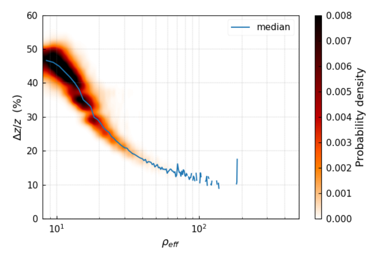
Figure 9 shows the distribution of relative error on the parameters of the detected compact binary system with the accumulated effective SNR. We see that the relative error drops with increasing . For it reduces from at to at . Figure 9b shows that the relative error redshift goes down from at to at . The respective errors for total mass , luminosity distance , and mass ratio are shown in Figs. 9c, 9d, 9e respectively.



VI.2.3 The effect of inclination on the recovery of parameters
The discussion in the previous section showed that sky localization has a dependence on the inclination angle of the detected compact binary system. It was shown in Fig. 8 that, for the detected compact binary sources located at , the sources with have a poor localization given the low SNR value. In addition to this, Fig. 10 shows the distribution of relative errors on and for all the detected sources with the sky localization. The left panels in Figs. 10a and 10b show the sources with or , and the right panels show the sources with . It can be seen that although only a few sources with generate enough SNR to be detected, the accuracy of recovered values of and for these low SNR cases, i.e square degrees, is better than for those with or . Most of the sources detectable with higher SNR and having better localization are the sources with the inclination angles or .


VI.2.4 The effect of choice of site on the localization capability of ET
We now proceed to test the localization capability of the ET for different orientations and at different sites. In order to see the affect of orientation of the detector on the sky localization, we assume that the ET is located at the Virgo site and repeat the analysis using the ET detector with three different orientations. The orientation is measured counterclockwise from East to the bisector of the interferometer arms. We assume the initial orientation to be and then analyze the same set of detected sources with the ET detector orientated at, and . Figure 11a shows the cumulative distribution of sky localization for these three different cases of orientation of the detector at the Virgo site. It can be concluded that the change in orientation does not have much effect on the sky localization.
We also investigate the change in the sky localization for different site locations of ET. We assume the locations to be in Maastricht and Sardinia in addition to the Virgo site. The coordinates of the sites are mentioned in Table 3. The site locations are chosen keeping in mind that these are the official candidate sites for the ET. The cumulative distributions of sky localization for these locations are shown in Fig. 11b and show no change in the effective sky localization.


VI.2.5 Biases in recovery of the parameters of the binary
In order to check the accuracy of the algorithm in recovering the distributions of the binary parameters, we show the recovered median values of the distributions with respect to source values for chirp mass , redshift , and total mass in Fig. 12. The blue contour in the plots encloses the 90% probability region.
Figure 12a shows the distribution of recovered median values of the intrinsic chirp mass with respect to the actual source value values. It is seen that the chirp masses are recovered correctly over the whole range of source values.
In the case of the median values of the redshift distribution, shown in Fig. 12b, we see that all cases detected with are slightly underestimated. This can be explained due to the low SNR generated by these sources and, hence, the larger error associated with the SNR as per our prior assumption. A more detailed explanation of the origin of this bias is given in the Appendix.
Figure 12c shows the recovered median vs source value for the total mass . We see that the recovered median values are overestimated over the whole range of source values. As mentioned earlier, we assume that , which gives the value of redshifted total mass, is measured accurately. Since redshift is underestimated, we see the overestimation in the recovered total mass values.
VII Conclusion
In this analysis, we studied the ability of ET as a single instrument to study longer-duration signals from coalescing low mass compact binary systems. We assume the detector to be located at the Virgo site and analyze the signal every 5 min, assuming that the response functions for the three ET detectors do not change much within that period.
We show that, although one cannot use time of flight delays to constrain the position in the sky of a given source in case of three co-located detectors in single ET, combining information from different antenna patterns for each of the three detectors in each time segment provides good constraints on the parameters of a merging binary system.
We analyzed a mock population of compact binary sources for which the signal will stay for a long duration in the ET detection band. Assuming that the change in the response functions is negligible within 5 min, we divided the inspiral signal into 5 min segments from the time it enters the detection band of ET at 1Hz with the duration of the last segment limited by , the frequency at the end of the inspiral.
We assumed the threshold of detection to be for the segment in the detector in at least one segment, for corresponding to the three ET detectors comprising single ET and the accumulated effective SNR .
The angles describing the location of the source, its inclination and polarization are constrained using the ratios of the SNRs generated in each signal segment of the three detectors of the equilateral triangle configuration of ET. This, in turn, provide constraints on the antenna response function in the segment.
We then use the information about , and initial and final GW frequency in segment to estimate the parameter . Combining the information about the angles from each segment increases the accuracy of the estimate of the angles and also gives a stricter constraint on . We then use the constraint on to estimate intrinsic chirp mass , redshift , total mass , luminosity distance , and mass ratio of the merging binary system.
We conclude that the ET as a single instrument can localize the low mass compact binary sources and break the chirp mass - redshift degeneracy. The analysis presented here allows us to estimate source frame masses and redshifts of the coalescing compact binaries which facilitates the population study of compact object binaries Singh et al. 2022.
We find that the accuracy of determination of the redshift and the source frame chirp mass with ET as a single instrument, is typically 40% and 20% , respectively for and it is and for . In the best case we see that using this method for analyzing a long-duration signal, single ET in triangular configuration can constrain the localization area for 90% probability region of to a minimum value of 7.68 square degrees, for , although only of binaries can be localized with 90% credibility, within 800 square degrees. It should be noted that the dominant error in the analysis is the one on the SNRs and our assumption of is a conservative one.
We also studied the effect of orientation of the detector on the sky localization with three different orientations of ET detector assumed to be located at the Virgo site and found that the change in orientation has no effect on the sky localization. In addition to this we also investigated the change in the sky localization for different site locations of ET. We assumed the location of ET to be in Maastricht and Sardinia in addition to Virgo, and found no change in the effective sky localization due to change in the ET site for these sites.
Acknowledgements.
We acknowledge the support from the Foundation for Polish Science Grant No. TEAM/2016-3/19 and NCN Grant No. UMO-2017/26/M/ST9/00978. N.S. is supported by the ”Agence Nationale de la Recherche”, Grant No. ANR-19-CE31-0005-01 (PI: F. Calore). We thank the anonymous reviewer for all the valuable comments and suggestions which helped us to improve the manuscript. This document has been assigned Virgo document number VIR-0785A-21.Appendix A Appendixes
In Fig. 12a, we see the deviation of the median value of the parameter from the true value of that parameter. This origin of this bias can be understood from the Fig. 13 which shows the distribution of defined in Eq. (6), assuming that the probability distributions of angular distribution , and , are uncorrelated and are distributed uniformly over the range . We see that this distribution of is inherently biased toward lower values. Therefore, for a given , defined in Eq. (9), the smaller has to be compensated by larger chirp mass and smaller redshift . Thus there is an inherent bias toward lower redshift and larger chirp mass.

One of the main building blocks of our analysis is that we use the ratios of SNRs in each segment for each of the three detectors in the triangular configuration of ET, to constrain the value of the effective antenna pattern. This is expressed in Eq. (26), assuming that the measurement error on the SNRs is Gaussian with the standard deviations for being . In Fig. 14, we show the absolute value of bias as the function of the ratio of the SNRs. We see that the estimate of parameters is likely to be biased for and . The reason for this can be understood by Fig. 13. We see that the distributions for , and are the same. So in the case of and , there is a much larger number of lower values of in the probability distribution constrained by these ratios of the SNRs. This results in smaller redshift and higher chirp mass in the respective distributions recovered for these parameters as explained above.

In order to see the variation in this bias due to the inclusion of segments of lower SNRs, we repeated the analysis for the following different detection criteria for 5-min segments.
- •
Criterion 1: A threshold value of accumulated effective SNR and the SNR for the segment in the detector in at least one segment. This is the criteria which we have used in our main analysis in this paper.
- •
Criterion 2: A threshold value of accumulated effective SNR and the SNR for the segment in the detector in at least one segment.
- •
Criterion 3: A threshold value of accumulated effective SNR and the SNR for the segment in the detector in at least one segment.
The recovered median values vs the actual source values of chirp mass and redshift, using these three detection criteria, are shown in Fig. 15. The left panel shows the comparison for the chirp mass, and the right panel shows the comparison for the redshift. The top panel shows the comparison of the estimated median value with respect to the actual value for criterion 1. When we repeat the analysis while including segments with , shown in the middle panel, we see that a few more sources cross the detection threshold and are shown in blue. The red points are the sources which were detectable with criterion 1, but their analysis now includes the additional low SNR segments. The bottom row shows the subsequent inclusion of segments of , thus detecting a few more sources, shown in blue. While lowering the detection threshold detects a few more sources, there is also a slight worsening of the bias as we include segments of lower SNRs in the analysis. This can be clearly seen from the red points as we go from the top panel to the bottom panel. The underestimation of redshift and the overestimate of chirp, are both slightly worsened.
Although the inclusion of segments of lower SNR worsens the bias, the error on the estimated parameters is lowered due to the additional information from these segments. The distribution of relative errors on chirp mass and redshift estimated using criterion 2 and criterion 3 are shown in Figure 16. Comparing these with the error estimates obtained using Criterion 1 shown in Fig. 9, we see that the additional segments contribute in reducing the relative errors, mainly for sources generating lower SNRs.


References
- Abbott et al. (2016) B. P. Abbott, R. Abbott, T. D. Abbott, M. R. Abernathy, F. Acernese, K. Ackley, C. Adams, T. Adams, P. Addesso, R. X. Adhikari, et al., Phys. Rev. Lett. 116, 061102 (2016), eprint 1602.03837.
- Abbott et al. (2021) R. Abbott, T. D. Abbott, S. Abraham, F. Acernese, K. Ackley, A. Adams, C. Adams, R. X. Adhikari, V. B. Adya, C. Affeldt, et al., Physical Review X 11, 021053 (2021), eprint 2010.14527.
- Abbott et al. (2019) B. P. Abbott, R. Abbott, T. D. Abbott, S. Abraham, F. Acernese, K. Ackley, C. Adams, R. X. Adhikari, V. B. Adya, C. Affeldt, et al. (LIGO Scientific Collaboration and Virgo Collaboration), Phys. Rev. X 9, 031040 (2019), URL https://link.aps.org/doi/10.1103/PhysRevX.9.031040.
- Abbott et al. (2020a) R. Abbott, T. D. Abbott, S. Abraham, F. Acernese, K. Ackley, C. Adams, R. X. Adhikari, V. B. Adya, C. Affeldt, M. Agathos, et al. (LIGO Scientific Collaboration and Virgo Collaboration), Phys. Rev. D 102, 043015 (2020a), URL https://link.aps.org/doi/10.1103/PhysRevD.102.043015.
- Abbott et al. (2020b) R. Abbott, T. D. Abbott, S. Abraham, F. Acernese, K. Ackley, C. Adams, R. X. Adhikari, V. B. Adya, C. Affeldt, M. Agathos, et al. (LIGO Scientific Collaboration and Virgo Collaboration), Phys. Rev. Lett. 125, 101102 (2020b), URL https://link.aps.org/doi/10.1103/PhysRevLett.125.101102.
- Abbott et al. (2017) B. P. Abbott, R. Abbott, T. D. Abbott, F. Acernese, K. Ackley, C. Adams, T. Adams, P. Addesso, R. X. Adhikari, V. B. Adya, et al. (LIGO Scientific Collaboration and Virgo Collaboration), Phys. Rev. Lett. 119, 161101 (2017), URL https://link.aps.org/doi/10.1103/PhysRevLett.119.161101.
- Goldstein et al. (2017) A. Goldstein, P. Veres, E. Burns, M. S. Briggs, R. Hamburg, D. Kocevski, C. A. Wilson-Hodge, R. D. Preece, S. Poolakkil, O. J. Roberts, et al., Astrophys. J. Lett. 848, L14 (2017), eprint 1710.05446.
- Savchenko et al. (2017) V. Savchenko, C. Ferrigno, E. Kuulkers, A. Bazzano, E. Bozzo, S. Brandt, J. Chenevez, T. J. L. Courvoisier, R. Diehl, A. Domingo, et al., Astrophys. J. Lett. 848, L15 (2017), eprint 1710.05449.
- Abbott et al. (2017a) B. P. Abbott, R. Abbott, T. D. Abbott, F. Acernese, K. Ackley, C. Adams, T. Adams, P. Addesso, R. X. Adhikari, V. B. Adya, et al., Astrophys. J. Lett. 848, L13 (2017a), eprint 1710.05834.
- Coulter et al. (2017) D. A. Coulter, R. J. Foley, C. D. Kilpatrick, M. R. Drout, A. L. Piro, B. J. Shappee, M. R. Siebert, J. D. Simon, N. Ulloa, D. Kasen, et al., Science 358, 1556 (2017), eprint 1710.05452.
- Troja et al. (2017) E. Troja, L. Piro, H. van Eerten, R. T. Wollaeger, M. Im, O. D. Fox, N. R. Butler, S. B. Cenko, T. Sakamoto, C. L. Fryer, et al., Nature 551, 71 (2017), eprint 1710.05433.
- Hallinan et al. (2017) G. Hallinan, A. Corsi, K. P. Mooley, K. Hotokezaka, E. Nakar, M. M. Kasliwal, D. L. Kaplan, D. A. Frail, S. T. Myers, T. Murphy, et al., Science 358, 1579 (2017), eprint 1710.05435.
- Abbott et al. (2017b) B. P. Abbott, R. Abbott, T. D. Abbott, F. Acernese, K. Ackley, C. Adams, T. Adams, P. Addesso, R. X. Adhikari, V. B. Adya, et al., Astrophys. J. Lett. 848, L12 (2017b), eprint 1710.05833.
- Hild et al. (2011) S. Hild, M. Abernathy, F. Acernese, P. Amaro-Seoane, N. Andersson, K. Arun, F. Barone, B. Barr, M. Barsuglia, M. Beker, et al., Classical and Quantum Gravity 28, 094013 (2011), eprint 1012.0908.
- Punturo et al. (2010) M. Punturo, M. Abernathy, F. Acernese, B. Allen, N. Andersson, K. Arun, F. Barone, B. Barr, M. Barsuglia, M. Beker, et al., Classical and Quantum Gravity 27, 194002 (2010).
- Dwyer et al. (2015) S. Dwyer, D. Sigg, S. W. Ballmer, L. Barsotti, N. Mavalvala, and M. Evans, Phys. Rev. D 91, 082001 (2015), URL https://link.aps.org/doi/10.1103/PhysRevD.91.082001.
- Abbott et al. (2017) B. P. Abbott, R. Abbott, T. D. Abbott, M. R. Abernathy, K. Ackley, C. Adams, P. Addesso, R. X. Adhikari, V. B. Adya, C. Affeldt, et al., Classical and Quantum Gravity 34, 044001 (2017), URL https://doi.org/10.1088%2F1361-6382%2Faa51f4.
- Reitze et al. (2019) D. Reitze, R. X. Adhikari, S. Ballmer, B. Barish, L. Barsotti, G. Billingsley, D. A. Brown, Y. Chen, D. Coyne, R. Eisenstein, et al., in Bulletin of the American Astronomical Society (2019), vol. 51, p. 35, eprint 1907.04833.
- Hild et al. (2008) S. Hild, S. Chelkowski, and A. Freise, arXiv e-prints arXiv:0810.0604 (2008), eprint 0810.0604.
- Hild (2012) S. Hild, Classical and Quantum Gravity 29, 124006 (2012), eprint 1111.6277.
- Huerta and Gair (2011a) E. A. Huerta and J. R. Gair, Phys. Rev. D. 83, 044020 (2011a), eprint 1009.1985.
- Huerta and Gair (2011b) E. A. Huerta and J. R. Gair, Phys. Rev. D. 83, 044021 (2011b), eprint 1011.0421.
- Gair et al. (2011) J. R. Gair, I. Mandel, M. C. Miller, and M. Volonteri, General Relativity and Gravitation 43, 485 (2011), eprint 0907.5450.
- Amaro-Seoane and Santamaría (2010) P. Amaro-Seoane and L. Santamaría, Astrophys. J. 722, 1197 (2010), eprint 0910.0254.
- Sathyaprakash et al. (2019) B. S. Sathyaprakash et al. (2019), eprint 1903.09260.
- Maggiore et al. (2020) M. Maggiore, C. Van Den Broeck, N. Bartolo, E. Belgacem, D. Bertacca, M. A. Bizouard, M. Branchesi, S. Clesse, S. Foffa, J. García-Bellido, et al., Journal of Cosmology and Astroparticle Physics 2020, 050 (2020), eprint 1912.02622.
- Regimbau et al. (2012) T. Regimbau, T. Dent, W. Del Pozzo, S. Giampanis, T. G. F. Li, C. Robinson, C. Van Den Broeck, D. Meacher, C. Rodriguez, B. S. Sathyaprakash, et al., Phys. Rev. D. 86, 122001 (2012), eprint 1201.3563.
- Regimbau et al. (2014) T. Regimbau, D. Meacher, and M. Coughlin, Phys. Rev. D. 89, 084046 (2014), eprint 1404.1134.
- Belgacem et al. (2019) E. Belgacem, Y. Dirian, S. Foffa, E. J. Howell, M. Maggiore, and T. Regimbau, Journal of Cosmology and Astroparticle Physics 2019, 015 (2019), eprint 1907.01487.
- Zhao and Wen (2018) W. Zhao and L. Wen, Phys. Rev. D. 97, 064031 (2018), eprint 1710.05325.
- Chan et al. (2018) M. L. Chan, C. Messenger, I. S. Heng, and M. Hendry, Phys. Rev. D. 97, 123014 (2018), eprint 1803.09680.
- Singh and Bulik (2021) N. Singh and T. Bulik, Phys. Rev. D. 104, 043014 (2021), eprint 2011.06336.
- Bulik et al. (2004) T. Bulik, K. Belczyński, and B. Rudak, Astron. Astrophys. 415, 407 (2004), eprint astro-ph/0307237.
- Jaranowski et al. (1998) P. Jaranowski, A. Królak, and B. F. Schutz, Phys. Rev. D 58, 063001 (1998), URL https://link.aps.org/doi/10.1103/PhysRevD.58.063001.
- Accadia et al. (2012) T. Accadia, F. Acernese, M. Alshourbagy, P. Amico, F. Antonucci, S. Aoudia, N. Arnaud, C. Arnault, K. G. Arun, P. Astone, et al., Journal of Instrumentation 7, 3012 (2012).
- Acernese et al. (2015) F. Acernese, M. Agathos, K. Agatsuma, D. Aisa, N. Allemandou, A. Allocca, J. Amarni, P. Astone, G. Balestri, G. Ballardin, et al., Classical and Quantum Gravity 32, 024001 (2015), eprint 1408.3978.
- Allen et al. (2012) B. Allen, W. G. Anderson, P. R. Brady, D. A. Brown, and J. D. E. Creighton, Phys. Rev. D. 85, 122006 (2012), eprint gr-qc/0509116.
- Sathyaprakash and Dhurandhar (1991) B. S. Sathyaprakash and S. V. Dhurandhar, Phys. Rev. D 44, 3819 (1991), URL https://link.aps.org/doi/10.1103/PhysRevD.44.3819.
- Taylor and Gair (2012) S. R. Taylor and J. R. Gair, Phys. Rev. D. 86, 023502 (2012), eprint 1204.6739.
- O’Shaughnessy et al. (2010) R. O’Shaughnessy, V. Kalogera, and K. Belczynski, Astrophys. J. 716, 615 (2010), eprint 0908.3635.
- Finn (1996) L. S. Finn, Phys. Rev. D. 53, 2878 (1996), eprint gr-qc/9601048.
- Maggiore (2007) M. Maggiore, Gravitational Waves. Vol. 1: Theory and Experiments, Oxford Master Series in Physics (Oxford University Press, 2007), ISBN 978-0-19-857074-5, 978-0-19-852074-0.
- The LIGO Scientific Collaboration et al. (2021) The LIGO Scientific Collaboration, the Virgo Collaboration, the KAGRA Collaboration, R. Abbott, T. D. Abbott, F. Acernese, K. Ackley, C. Adams, N. Adhikari, R. X. Adhikari, et al., arXiv e-prints arXiv:2111.03606 (2021), eprint 2111.03606.
- Aubourg et al. (2015) É. Aubourg, S. Bailey, J. E. Bautista, F. Beutler, V. Bhardwaj, D. Bizyaev, M. Blanton, M. Blomqvist, A. S. Bolton, J. Bovy, et al., Phys. Rev. D. 92, 123516 (2015), eprint 1411.1074.
- Adachi and Kasai (2012) M. Adachi and M. Kasai, Progress of Theoretical Physics 127, 145 (2012), eprint 1111.6396.
- Singh et al. (2022) N. Singh, T. Bulik, K. Belczynski, and A. Askar, Astron. Astrophys. 667, A2 (2022), eprint 2112.04058.
- Lattimer (2012) J. M. Lattimer, Annual Review of Nuclear and Particle Science 62, 485 (2012), eprint 1305.3510.