Generating Large-scale Dynamic Optimization Problem Instances Using the Generalized Moving Peaks Benchmark
Abstract
This document describes the generalized moving peaks benchmark (GMPB) [1] and how it can be used to generate problem instances for continuous large-scale dynamic optimization problems. It presents a set 15 benchmark problems, the relevant source code, and a performance indicator, designed for comparative studies and competitions in large-scale dynamic optimization. Although its primary purpose is to provide a coherent basis for running competitions, its generality allows the interested reader to use this document as a guide to design customized problem instances to investigate issues beyond the scope of the presented benchmark suite. To this end, we explain the modular structure of the GMPB and how its constituents can be assembled to form problem instances with a variety of controllable characteristics ranging from unimodal to highly multimodal, symmetric to highly asymmetric, smooth to highly irregular, and various degrees of variable interaction and ill-conditioning.
keywords
evolutionary dynamic optimization, tracking moving optimum, large-scale dynamic optimization problems, generalized moving peaks benchmark.1 Introduction
Change is an inescapable aspect of natural and artificial systems, and adaptation is central to their resilience. Optimization problems are no exception to this maxim. Indeed, viability of businesses and their operational success depend heavily on their effectiveness in responding to a change in the myriad of optimization problems they entail. For an optimization problem, this boils down to the efficiency of an algorithm to find and maintain a sequence of quality solutions to an ever changing problem.
Ubiquity of dynamic optimization problems (DOPs) [2] demands extensive research into design and development of algorithms capable of dealing with various types of change [3]. These are often attributed to a change in the objective function, its number of decision variables, or constraints. Despite the large body of literature on dynamic optimization problems and algorithms, little attention has been given to their scalability [4, 5]. Indeed, the number of dimensions of a typical DOP studied in the literature rarely exceeds twenty.
Motivated by rapid technological advancements, large-scale optimization has gained popularity in recent years [6]. However, the exponential growth in the size of the search space, with respect to an increase in the number of decision variables, has made large-scale optimization a challenging task. For DOPs, however, the challenge is twofold. For such problems, not only should an algorithm be capable of finding the global optimum in the vastness of the search space but it should also be able to track it over time. For multi-modal DOPs, where several optima have the potential to turn into the global optimum after environmental changes, the cost of tracking multiple moving optima also adds to the complexity.
Real-world large-scale optimization problems often exhibit a modular structure with nonuniform imbalance among the contribution of its constituent parts to the objective value [7, 8]. The modularity is caused by the interaction structure of the decision variables resulting in a wide range of structures from fully separable functions to fully nonseparable ones. Most problems exhibit some degree of sparsity in their interaction structure, which can be exploited by optimization algorithms. The imbalance property can be caused as a by-product of modularity or due to the heterogeneous nature of the input variables and their domains.
Generalized moving peaks benchmark (GMPB) [1] is capable of generating problem instances with a variety of characteristics that can range from fully non-separable to fully separable structure, from homogeneous to highly heterogeneous sub-functions, and from balanced to highly imbalanced sub-functions. Each sub-function generated by GMPB is constructed by assembling several components. In most benchmark generators in the filed of DOPs, these components are unimodal, smooth, symmetric, fully separable, and easy-to-optimize peaks. However, GMPB is capable of generating components with a variety of properties that can range from unimodal to highly multimodal, from symmetric to highly asymmetric, from smooth/regular to highly irregular, with different variable interaction degrees, and from low condition number to highly ill-conditioned.
2 Generalized Moving Peaks Benchmark [1, 9]
GMPB’s main function is constructed by assembling several sub-functions as follows:
| (1) |
where shows the current environment number, is the th sub-function in the th environment, is the number of sub-functions, is the dimension of the main function, is the dimension of the sub-function , and controls the contribution of sub-function for generating imbalance property. The baseline function that generates each sub-function in GMPB is:
| (2) |
where is calculated as [10]:
| (3) |
where is a subset of decision variables (-dimensional) of the solution , which belongs to the th sub-function, is the number of components in , is the rotation matrix of the th component of the th sub-function in the th environment, is a diagonal matrix whose elements determine the width of the th component in different dimensions, is th element of , and and are irregularity parameters of the th component of the th sub-function.
For each component of the th sub-function, the rotation matrix is obtained by rotating the projection of onto all - planes by a given angle . The total number of unique planes which will be rotated is . For rotating each - plane by a certain angle (), a Givens rotation matrix, , must be constructed. To do this, is first initialized to an identity matrix ; then, four elements of are altered as follows:
| (4) |
Thus, the rotation matrix, , in the th environment is calculated as follows:
| (5) |
where contains all unique pairs of dimensions defining all possible planes in a -dimensional space. The order of the multiplications of the Givens rotation matrices is random. The reason behind using (5) for calculating is that we aim to have control on the rotation matrix based on an angle severity . Note that the initial for problem instances with rotation property is obtained by using the Gram-Schmidt orthogonalization method on a matrix with normally distributed entries.
For each component in the th sub-function, the height, width vector, center, angle, and irregularity parameters change from one environment to the next according to the following update rules:
| (6) | ||||
| (7) | ||||
| (8) | ||||
| (9) | ||||
| (10) | ||||
| (11) |
where is a random number drawn from a Gaussian distribution with mean 0 and variance 1, shows the vector of center position of the th components of the th sub-function, is a -dimensional vector of random numbers generated by , is the Euclidean length (i.e., -norm) of , generates a unit vector with a random direction, , , , , and are height, width, shift, angle, and irregularity parameters’ change severity values of components in the h sub-function, respectively, 11 1 Not to be confused with that controls the components’ imbalance. shows the width of the th component in the th dimension of the th sub-function, and and show the height and angle of the th component in the th sub-function, respectively.
Outputs of equations (6) to (11) are bounded as follows: , , , , , and , where and are maximum and minimum problem space bounds in the th sub-function. For keeping the above mentioned values in their bounds, a Reflect method is utilized. Assume represents one of the equations (6) to (11). The output based on the reflect method is:
| (12) |
2.1 Characteristics of the components, sub-functions, and problem instances
In this section, we describe the main characteristics of the components, sub-functions, and problem instances generated by GMPB.
2.1.1 Component characteristics
In the simplest form, (2) generates a symmetric, unimodal, smooth/regular, and easy-to-optimize conical peak (see Figure 1). By setting different values to and , a component generated by GMPB becomes irregular and multimodal. Figure 2 shows two irregular and multimodal components generated by GMPB with different parameter settings for and . The illustrated component in Figure 2(a) is easier to optimize in comparison to the one shown in Figure 2(c). As can be seen in Figure 2(d), the local optima on the basin of attraction of the component are very vast which results in premature convergences. The results shown in the supplementary document of [1] indicate that the performance of the optimization algorithms such as the particle swarm optimization (PSO) [11] and differential evolution (DE) [12] deteriorates significantly in such components. A component is symmetric when all values are identical, and components whose values are set to different values are asymmetric (see Figure 3).


GMPB is capable of generating components with various condition numbers. A component generated by GMPB has a width value in each dimension. When the width values of a component are identical in all dimensions, the condition number of the component will be one, i.e., it is not ill-conditioned. The condition number of a component is the ratio of its largest width value to its smallest value [1]. If a component’s width value is stretched in one axis’s direction more than the other axes, then, the component is ill-conditioned. Figure 4 depicts three components with different condition numbers.


In GMPB, each component is rotated using . If , then the component is not rotated (See Figure 5(a)). Figure 5(c) shows the component from Figure 5(a) which has been rotated by . In GMPB, by changing over time using (9), the variable interaction degrees of the th component change over time.


2.1.2 Sub-function characteristics
In GMPB, a sub-function is constructed by assembling several components using a function in (2), which determines the basin of attraction of each component. As shown in [4], the landscape made by several components (i.e., ) by the function is fully non-separable. Figure 6 shows a landscape with three components.
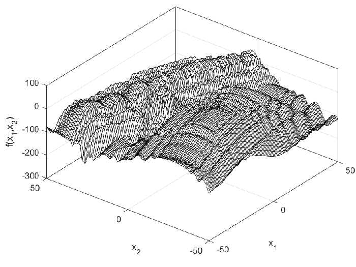

2.1.3 Problem characteristics
A problem instance generated by GMPB is modular and constructed by assembling several sub-functions using (1). These problems can be heterogeneous since the sub-functions can have different characteristics, such as different number of components, dimension, global optimum position, and change intensity. Besides, by assigning different weight values to each sub-function (), the problems can exhibit imbalance among its components. In an imbalanced problem, the contributions of sub-functions on the overall fitness value are different. Consequently, some sub-functions become more important for the optimization algorithms [13].
A consequence of GMPB’s design is the exponential growth in the total number of promising regions that can contain the global optimum in a future environment. In each GMPB’s sub-function, the total number of such promising regions can be up to the number of components whose center position can become the global optimum after environmental changes. However, by assembling several sub-functions using (1), the number of such promising regions in the problem becomes:
| (13) |
where is the number of components in the th sub-function. It should be noted that is the maximum number of promising regions that can exist in the landscape, which may change over time due to coverage of smaller components by larger ones. For the sake of clarity, we provide an illustrative example. In Figure 7(a) and Figure 7(b), two 1-dimensional sub-functions with two and three components (in the simplest form, i.e., conical peaks) are shown. The 2-dimensional function constructed based on (1) with results in a total of promising regions.


3 Problem instances
We present 15 GMPB large-scale scenarios with five different variable interaction structures in 50-, 100-, and 200-dimensional spaces, which are shown in Table 1. Note that in dynamic environments, the curse of dimensionality happens in much lower dimensions in comparison to static optimization problems [4]. In fact, the very limited available computational resources (i.e., the number of fitness evaluations) in each environment of DOPs results in a significant deterioration in the performance of locating and tracking the moving global optimum even in problems with 50-dimensional search space.
In the presented 15 GMPB large-scale scenarios in Table 1, the number of dimensions of the main function () in (1) and all sub-functions (), and also the variable interaction structures of the main function are fixed and do not change over time. The order of components in the actual benchmarks is taken from a random permutation; however, in Table 1 we present them in sorted order for better readability. Every fitness evaluations, the center position, height, width vector, angle, and irregularity parameters of each component in each sub-function change using the dynamics presented in (6) to (11). The parameter settings of each sub-function (2) including their change severity values (in (6) to (11)) and their ranges are listed in Table 2. Besides, the temporal parameter settings are shown in Table 3. Finally, Table 4 shows the initial values of the components’ parameters.
The problem instances can become more difficult by setting some parameters to what we call challenging settings. These challenging settings are characterized as follows. By increasing the shift severity values, optima relocate more severely and tracking them will become more time-consuming. Increasing the number of components results in a larger number of promising regions that may contain the global optimum after environmental changes. Therefore, dynamic optimization algorithms (DOAs) that try to locate and track multiple moving promising regions [14] will face difficulties in tackling such problems. In fact, covering larger numbers of promising regions is more computational resource consuming which is challenging due to the limited available computational resources in each environment. Another factor to increase the difficulty of each sub-function is to set all irregularity parameters’ boundaries to the challenging settings. This parameter setting results in larger plateau (See Figure 2), which significantly increases the probability of premature convergence. Finally, by decreasing the value of , we can increase the change frequency (see Table 3). In problem instances with higher change frequencies, the available computational resources in each environment (i.e., the number of fitness evaluations in each environment) are more limited which results in increased difficulty.
| Function | Dimensionality of Nonseparable Components | # Separable Vars | |
|---|---|---|---|
| 50 | 10 | ||
| 50 | 35 | ||
| 50 | 0 | ||
| 50 | — | 50 | |
| 50 | 0 | ||
| 100 | 20 | ||
| 100 | 70 | ||
| 100 | 0 | ||
| 100 | — | 100 | |
| 100 | 0 | ||
| 200 | 50 | ||
| 200 | 130 | ||
| 200 | 0 | ||
| 200 | — | 200 | |
| 200 | 0 |
| Parameter | Symbol | Default setting | Challenging setting |
|---|---|---|---|
| Shift severity | |||
| Numbers of components | |||
| Angle severity | - | ||
| Height severity | - | ||
| Width severity | - | ||
| Irregularity parameter severity | - | ||
| Irregularity parameter severity | - | ||
| Weight of sub-function | - | ||
| Search range | - | ||
| Height range | - | ||
| Width range | - | ||
| Angle range | - | ||
| Irregularity parameter range | - | ||
| Irregularity parameter range | - |
| Parameter | Symbol | Default setting | Challenging setting |
|---|---|---|---|
| Change frequency | |||
| Number of Environments | 30 | - |
| Parameter | Symbol | Initial value |
|---|---|---|
| Center position | ||
| Height | ||
| Width | ||
| Angle | ||
| Irregularity parameter | ||
| Irregularity parameter | ||
| Rotation matrix |
-
is initialized by performing the Gram-Schmidt orthogonalization method on a matrix with normally distributed entries.
4 Performance indicator
To measure the performance of DOAs in solving the problem instances generated by GMPB, the average error of the best found solutions at the end of all environments (i.e., the best before change error ()) is used as the performance indicator [15]:
| (14) |
where is the best found position in the th environment which is fetched at the end of the environment, is (1), is the maximum height value among the components of the th sub-function in the th environment, and calculates the global optimum fitness value in the th environment.
5 Source code
The MATLAB22 2 Version R2019a source code of the large-scale scenarios generated by the GMPB can be downloaded from [16]. As a sample optimization algorithm, we have added to this code as the optimizer. is a cooperative coevolutionary algorithm, which has been designed to tackle large-scale DOPs [4]. This algorithm uses the DG2 [8] for decomposing the problem and identifying the variable interaction structure of the problem. Thereafter, each sub-function is assigned to a multi-population PSO algorithm which work cooperatively via a context vector [17].
References
- [1] D. Yazdani, M. N. Omidvar, R. Cheng, J. Branke, T. T. Nguyen, and X. Yao, “Benchmarking continuous dynamic optimization: Survey and generalized test suite,” IEEE Transactions on Cybernetics, pp. 1 – 14, 2020.
- [2] D. Yazdani, R. Cheng, D. Yazdani, J. Branke, , Y. Jin, and X. Yao, “A survey of evolutionary continuous dynamic optimization over two decades – part A,” IEEE Transactions on Evolutionary Computation, 2021.
- [3] T. T. Nguyen, S. Yang, and J. Branke, “Evolutionary dynamic optimization: A survey of the state of the art,” Swarm and Evolutionary Computation, vol. 6, pp. 1 – 24, 2012.
- [4] D. Yazdani, M. N. Omidvar, J. Branke, T. T. Nguyen, and X. Yao, “Scaling up dynamic optimization problems: A divide-and-conquer approach,” IEEE Transaction on Evolutionary Computation, 2019.
- [5] D. Yazdani, R. Cheng, D. Yazdani, J. Branke, , Y. Jin, and X. Yao, “A survey of evolutionary continuous dynamic optimization over two decades – part B,” IEEE Transactions on Evolutionary Computation, 2021.
- [6] S. Mahdavi, M. E. Shiri, and S. Rahnamayan, “Metaheuristics in large-scale global continues optimization: A survey,” Information Sciences, vol. 295, pp. 407–428, 2015.
- [7] M. N. Omidvar, X. Li, and K. Tang, “Designing benchmark problems for large-scale continuous optimization,” Information Sciences, vol. 316, pp. 419–436, 2015.
- [8] M. N. Omidvar, M. Yang, Y. Mei, X. Li, and X. Yao, “DG2: A faster and more accurate differential grouping for large-scale black-box optimization,” IEEE Transactions on Evolutionary Computation, vol. 21, no. 6, pp. 929–942, 2017.
- [9] D. Yazdani, J. Branke, M. N. Omidvar, C. Li, M. Mavrovouniotis, T. T. Nguyen, S. Yang, and X. Yao, “Generalized moving peaks benchmark,” arXiv preprint arXiv:2106.06174, 2021.
- [10] N. Hansen, S. Finck, R. Ros, and A. Auger, “Real-parameter black-box optimization benchmarking 2009: Noiseless functions definitions,” INRIA, Tech. Rep. RR-6829, 2010.
- [11] J. Kennedy and R. Eberhart, “Particle swarm optimization,” in Proceedings of ICNN’95-International Conference on Neural Networks, vol. 4. IEEE, 1995, pp. 1942–1948.
- [12] J. Brest, S. Greiner, B. Boskovic, M. Mernik, and V. Zumer, “Self-adapting control parameters in differential evolution: A comparative study on numerical benchmark problems,” IEEE Transactions on Evolutionary Computation, vol. 10, no. 6, pp. 646–657, 2006.
- [13] D. Yazdani, “Particle swarm optimization for dynamically changing environments with particular focus on scalability and switching cost,” Ph.D. dissertation, Liverpool John Moores University, Liverpool, UK, 2018.
- [14] D. Yazdani, R. Cheng, C. He, and J. Branke, “Adaptive control of sub-populations in evolutionary dynamic optimization,” IEEE Transactions on Cybernetics, pp. 1 – 14, 2020.
- [15] K. Trojanowski and Z. Michalewicz, “Searching for optima in non-stationary environments,” in Congress on Evolutionary Computation, vol. 3, 1999, pp. 1843–1850.
- [16] D. Yazdani, Using PSO-CTR for Solving Large-Scale Generalized Moving Peaks Benchmark (MATLAB Source Code), 2021 (accessed June 11, 2021). [Online]. Available: https://bitbucket.org/public-codes-danial-yazdani/pso_ctr-for-large-scale-gmpb/src/main/
- [17] F. van den Bergh and A. P. Engelbrecht, “A cooperative approach to particle swarm optimization,” IEEE Transactions on Evolutionary Computation, vol. 8, no. 3, pp. 225–239, 2004.