AJB-21-4
BARI-TH/21-729
The charm of 331
Andrzej J. Burasa, Pietro Colangelob, Fulvia De Faziob and
Francesco Loparcob,c
aTUM Institute for Advanced Study, Lichtenbergstr. 2a, D-85747 Garching, Germany
bIstituto Nazionale di Fisica Nucleare, Sezione di Bari, Via Orabona 4,
I-70126 Bari, Italy
cDipartimento Interateneo di Fisica ”Michelangelo Merlin”, Università degli Studi di Bari, via Orabona 4, 70126 Bari, Italy
Abstract
We perform a detailed analysis of flavour changing neutral current processes in the charm sector in the context of 331 models. As pointed out recently, in the case of contributions in these models there are no new free parameters beyond those already present in the and meson systems analyzed in the past. As a result, definite ranges for new Physics (NP) effects in various charm observables could be obtained. While generally NP effects turn out to be small, in a number of observables they are much larger than the tiny effects predicted within the Standard Model. In particular we find that the branching ratio of the mode , despite remaining tiny, can be enhanced by 6 orders of magnitude with respect to the SM. We work out correlations between this mode and rare and decays. We also discuss neutral charm meson oscillations and CP violation in the charm system. In particular, we point out that 331 models provide new weak phases that are a necessary condition to have non-vanishing CP asymmetries. In the case of , the difference between the CP asymmetries in and , we find that agreement with experiment can be obtained provided that two conditions are verified: the phases in the ranges predicted in 331 models and large hadronic matrix elements.
1 Introduction
The role of charm in particle physics can hardly be overemphasized[1]. Not only historically the discovery of , and hence of the charm quark, was so important to be ascribed the name of November revolution, but even in much more recent times, the observation of charmed states with properties not expected in the quark model requires the development of a new hadron spectroscopy, to incorporate all hints of exotic states in a predictive framework.
However, the peculiar role of charm brings in also difficulties from the theory point of view. The first reason lies in the fact that the charm quark is not as heavy as the beauty quark to allow a completely reliable use of the heavy quark techniques efficiently developed for beauty hadrons. On the other hand, it cannot either be considered a light quark, so that the theoretical predictions are very often affected by uncertainties difficult to control because of long distance dynamics.
Among the observables in the charm sector showing this kind of problems there are the neutral meson mixing, i.e. oscillation, and CP violation, as well as rare charm decays governed by penguin diagrams [2]. Two facts make the Standard Model (SM) treatment of these processes rather challenging. The first one is that loop-induced processes in the charm case get contributions from internal down-type quarks. Since the loop functions depend on the ratios , the smallness of these ratios for makes them all very close to zero and therefore almost equal, resulting in almost perfect GIM cancellation. Another point is that the CKM elements involving charm have tiny imaginary parts, which is a challenge for CP violation studies if the SM was the whole story. Yet, we know that the SM is not the whole story. Hence, the strong suppression of some processes within SM, namely lepton flavour violating decays and the electric dipole moments, can even be an advantage in the search for new physics (NP) because of the small SM background. In the case of rare flavour changing neutral current (FCNC) processes induced by the transition the effectiveness of the GIM mechanism results in so tiny branching ratios in the SM that one can consider them as null tests: their observation with a less severe degree of suppression with respect to SM would be a signal of NP.
Deviations from the SM predictions in the flavour sector have been observed in several cases: they are usually referred to as flavour anomalies. Such tensions deal with loop-induced processes, as in the ratios and in the so-called distribution in processes, and very recently in . They also affect tree-level charged current processes, as in the ratios in semileptonic decay and in the analogous ratios involving corresponding decays of other beauty hadrons [3, 4]. In view of this, it is natural to look for deviations in other processes, and the purpose of this paper is to explore possible deviations from the SM expectations in the charm sector. A SM extension that could be promising from this point of view is the 331 model, whose main features we briefly describe in the next Section. The reason is the presence in this model of a new neutral gauge boson that can mediate tree-level FCNC. A few new parameters are introduced, affecting the interaction Lagrangian of SM fermions with . As observed in [5], it is remarkable that the parameters governing the flavour violating coupling , which enter in FCNC charm transitions, up to CKM factors are the same parameters describing the and couplings. This is a rather powerful feature: it allows us to exploit the experimental constraints in the kaon and in the beauty systems to place bounds on rare charm transitions and to establish correlations among observables in the three sectors.
The plan of the paper is the following. In Section 2 we present the basic features of the 331 model and of its variants. Section 3 is devoted to mixing, CP violation and rare charm decays in the SM and in 331 models. The numerical results and the correlations with kaon and observables are presented in Section 4. In the last Section we summarize our findings.
2 331 model
The extension of the SM gauge group to , proposed in [6, 7], defines a class of models generically referred to as 331 models. In these models two spontaneous symmetry breakings occur: first to the SM group and then to . The larger group leads to the introduction of 5 additional gauge bosons, as well as new fermions. Indeed, with the enlargement the left-handed SM fermions are components of triplets or antitriplets rather than doublets. As a consequence, a third partner is usually needed, in general a new heavy fermion.
A very appealing feature of 331 models is that the requirement of anomaly cancelation together with that of asymptotic freedom of QCD constrains the number of generations to be equal to the number of colours, making the 331 able to predict the existence of just three generations of ordinary quarks11 1 This is not possible within the SM unless other constraints like the width of Higgs are taken into account.. Moreover, quark generations should transform differently under the action of . In particular, two quark generations should transform as triplets, one as an antitriplet. The common choice is that the latter is the third generation. The different role of the third generation with respect to the others could possibly be at the origin of the large top quark mass.
The relation
| (1) |
between the electric charge and and , two of the generators, and , the generator of , introduces a parameter . This is a key parameter that defines the specific variant of the model. Among the new gauge bosons, four of them and have properties that depend on the value of : they have integer charges when is multiple of and of . On the other hand, in all the model variants a new neutral gauge boson is present. A very appealing feature of the 331 models is that mediates tree-level flavour changing neutral currents in the quark sector, while its couplings to leptons are diagonal and universal. An extended Higgs sector also comprises three triplets and one sextet. Finally, a relation exists between the gauge coupling and the coupling :
| (2) |
where is the Weinberg angle.
In analogy to the SM, quark mass eigenstates are obtained through rotation of flavour eigenstates by means of two unitary matrices (for up-type quarks) and (for down-type ones) that satisfy the relation , as in the SM case. However, while in the SM appears only in charged current interactions and and never appear individually, in the 331 models it is possible to get rid of only one matrix, or , by expressing it in terms of and the other one; the remaining rotation matrix enters in the couplings to quarks. Choosing as the surviving rotation matrix, one can parametrize it as [8]
| (3) |
In the 331 Lagrangian density the term describing the interaction with ordinary fermions reads:
| (4) | |||||
where , denotes an up (down)-type quark ( are generation indices), and , are the elements of the and matrices, respectively.
Using the parametrization in Eq. (3) and the Feynman rules for couplings to quarks from Eq. (4) [8, 9], one finds that the system involves only the parameters and , while the system involves only and . Kaon physics depends on , and , so that stringent correlations between observables in sectors and in the kaon sector can be established.
Exploiting this feature, correlations among several quark flavour observables in , and decays have been studied in [8, 9, 10, 11, 12]. Moreover, the relation
| (5) |
produces additional correlations between decays and the transitions induced by up-type quark FCNC decays mediated by , which occur in 331 models. In particular, as it follows from Eq. (4), correlations exist between observables in the charm sector and observables for , and . This observation has been exploited to relate the processes, such as , to processes induced by and [5]. Here we focus on other important processes in the charm sector.
As shown in Ref.[9], the variants of the model with and , with the fermions in the third generation transforming as antitriplets, satisfy a number of phenomenological constraints, such as those from observables in the systems, as well as the electroweak precision observables, provided that the mass of is not smaller than about TeV. Among such variants, the one with (denoted as M8 in [11]) predicts relevant contributions to the ratio [11].
Another remark concerns the mixing in this model [10]. The mixing can be neglected in the case of transitions and in decays like , where they are suppressed by the small vectorial coupling of to charged leptons. However, the contributions of tree-level exchanges to decays sensitive to axial-vector couplings, namely , and those with neutrinos in the final state, cannot be neglected, in general. The mixing angle can be written as [10]:
| (6) |
where
| (7) |
The parameter introduced in Eq. (6) is defined in terms of the vacuum expectation values of two Higgs triplets and , as follows:
| (8) |
| (9) |
With the same notation of the two Higgs doublet models, is expressed in terms of the parameter as 22 2 The overline distinguishes from the parameter characterizing the 331 models.:
| (10) |
A detailed analysis of the impact of the mixing in several 331 models distinguished by different values of , including the constraints from electroweak precision observables, is presented in [10]. Here, we analyze the impact on the charm sector, in particular on mixing, on CP violation in system and on rare transitions 33 3 The mass difference in the neutral D system has been studied in 331 models with considering the contribution to FCNC of the mixing between ordinary and exotic quarks [13]. The effects of new scalars have been investigated in [14], while FCNC processes in 331 models with right-handed neutrinos have been considered in [15]. .
3 Charm observables in the SM and in 331 model
3.1 mixing and
Neutral charmed mesons provide the only system where flavour oscillation of up-type quarks can occur. The time evolution of the system is governed by a Schrödinger equation:
| (11) |
Due to off-diagonal terms in , mass eigenstates do not coincide with the flavour eigenstates , but are given by
| (12) | |||||
| (13) |
with
| (14) |
CP parity transforms into each other modulo a phase that can be chosen in such a way that
| (15) |
Mass and width differences are usually normalized to the average width of the two mass eigenstates:
| (16) |
with
| (17) | |||||
| (18) |
In the 2021 online report the HFLAV group quoted the summary of the charm-mixing data obtained from global fits in which CP violation is allowed [16]:
| (19) | |||||
| (20) |
New measurements have been provided by the LHCb collaboration allowing for CP violation in mixing and in the interference between mixing and decay. The best fit point is [17]:
| (21) | |||||
| (22) |
It appears then that in the system or , whereas in the system . For future prospects see [18, 19]. In the limit of (approximate) CP symmetry , implies that the CP even state () is slightly heavier and shorter lived than the CP odd one () (unlike for neutral kaons).
In the SM the mixing originates in the box diagrams with exchange and internal down-type quarks, as opposed to and mixings where the up-type quarks are exchanged, in particular the top-quark. As a result, the mass differences predicted by the SM turn out to be in the ballpark of their experimental values. This also holds for , although in this case sizable long-distance contributions are present which are still not fully under control [19].
As in the case of and mixings, the short-distance contribution to mixing in the SM is governed by a single operator , so that this contribution can be easily evaluated. One finds that, due to strong GIM suppression, and are by at least one order of magnitude below the experimental values in (19), so that either long-distance or new physics contributions are responsible for their measured values.
Many predictions for in the SM have been worked out, which however are affected by large uncertainties, as discussed in Section 3 of [19]. As in the SM, corresponds to the dispersive part and to the absorptive part of the box diagrams, which are both strongly suppressed by the GIM mechanism. The short-distance SM contributions to them are both real to a very good approximation, and this is also the case of the long-distance contributions. This implies that, unless NP contributions to and in a given model are in the ballpark of their values in (19), the best chance to search for NP in mixing is through CP violation, represented by the departure of from unity and the non-vanishing phase in the measured range in (20).
If NP is taken into account, other operators beyond can contribute. The experimental values in (19) and (20) provide strong constraints to the extensions of the SM in which left-right, scalar and tensor operators are present [20, 21, 22, 23]. Indeed, such operators have large hadronic matrix elements and strongly enhanced Wilson coefficients through QCD renormalization group effects,
In the 331 model only the operator is involved, as in the SM, but this time its Wilson coefficient receives the contribution from tree-level exchange. However, even such tree-level contributions are below the experimental values of and when the contraints from the other quark sectors are included. As a matter of fact in the 331 model, if all other contributions to the mixing are ignored, at the scale is given by:
| (23) |
where is the decay constant and parametrizes the deviation of the matrix element of the four quark operator from the vacuum saturation approximation. The coupling reads:
| (24) |
The elements can be obtained using Eqs. (3) and (5):
| (25) | |||||
| (26) |
Hence, depends on the four parameters and which govern and decays, respectively, and which altogether govern the decays.
When evolved down to , the RG running gives [24, 25]:
| (27) |
with
| (28) |
The evolution can be performed including NLO QCD corrections by means of the results in [26], but here we restrict the analysis to the leading order. The reason is that, as discussed in Section 4, the numerical value of resulting from (23),(27) is below the experimental measurement in (19) by about one order of magnitude when the constraints on , , and are considered.
The small value of leads us to conjecture that both SM long-distance and 331 contributions are responsible for the measured values of and . The 331 term is pivotal in providing the complex phases producing a deviation of from unity and a non-vanishing mixing phase . This is at the basis of the analysis strategy in Section 4: We use the measured values of and in Eq. (19), interpreting them as resulting from the contributions of both LD in the SM and of 331. Then, we predict observables and correlations, as those involving and .
3.2 CP asymmetries
CP violation in the charm system can be tested in various ways. Here we consider the time-dependent CP asymmetries
| (29) |
where is a CP eigenstate
| (30) |
Denoting , we define
| (31) |
The phase is phase-convention independent since it depends only on the relative phase between and :
| (32) |
where if and if .
In the case of a non-negligible CP phase in the decay amplitude , but , simplifies to
| (33) |
In this case, as , it is appropriate to consider the CP asymmetry in the limit of a small [27]:
| (34) |
where .
On the other hand, when the phase is negligible, as happens in the SM and, as we shall see, also in the 331 models, one has
| (35) |
and
| (36) |
with
| (37) |
is analogous to and in the and system, respectively. However, in the system and , so that the above result simplifies considerably, leaving only the second term and allowing the measurement of the phase .
Finally, we consider the semileptonic asymmetry to wrong sign leptons
| (38) |
with , which represents CP violation in mixing in transitions. The last expression comes from the condition .
3.3 Correlations
Two interesting correlations have been derived in [28], which read with our conventions [27]:
| (39) |
In the limit , , the relation (39) simplifies to [28]
| (40) |
Inserting this result in (37) and (38) one finds for :
| (41) |
It should be emphasized that this relation is only valid if in our convention independently of , that is no CP phase in decay amplitudes. The experimental violation of the relation (41) would then imply the occurrence of CP violation in the decay (direct CP violation) [28]. In the case of a significant phase one finds:
| (42) |
As is phase convention dependent, the presence of direct CP violation would be signalled by finding for two different final states and .
We shall analyze all these relations within 331 models in Section 4, but we want to have first a look at time-independent CP-asymmetries.
3.4
The first observation of CP violation in the decays of neutral charm mesons was presented by the LHCb collaboration. For the difference between the CP asymmetries in and ,
| (43) |
the measurement is [29]
| (44) |
With an excellent approximation this difference measures direct CP violation. Within the SM this result has been explained invoking non perturbative effects enhancing the penguin contributions [30, 31, 32, 33, 34, 35, 36, 37, 38, 39, 40]. Other studies envisage the possibility that some NP could be responsible for this result [41, 42, 43, 44, 45, 46, 47, 48] (also supported by the analysis in [49]). A discussion of the LHCb data and of the future prospects can be found in [2]. Here we analyze the asymmetry in 331 models.
The modes and are single Cabibbo suppressed. These are of the kind with a CP eigenstate that can be produced both in and decays. Denoting , and CP (), the CP asymmetry is defined as
| (45) |
Note that in contrast to (29) this asymmetry is time-independent.
When two amplitudes (at least) contribute to each decay, one can write [31]
| (46) |
where and , are the difference between strong and weak phases, respectively. If one of the amplitudes dominates, i.e. , one finds:
| (47) |
When NP is present the previous relations can be generalized by adding a new amplitude to (46):
| (48) |
with and , . Consequently we have:
| (49) |
In the SM both and have a tree-level contribution , proportional to for and to for . Penguin contributions are also present with internal down-type quark exchange and hence proportional to with . We denote such contributions as . Exploiting the CKM unitarity relation , the general structure of the SM amplitude reads:
| (50) | |||||
| (51) |
In 331 models new contributions from tree-level exchanges are present. Except for different hadronic matrix elements and the change of the coupling to given in Eq. (24), the structure of the contribution to the effective Hamiltonian at is as in the case of the ratio [10]. While flavour-changing couplings involve only left-handed quarks, flavour conserving ones involve both left and right-handed ones. Flavour conserving couplings to left-handed quarks are
| (52) | |||||
| (53) |
with given in (7). Numerically, the second term in Eqs. (52)-(53) is a factor of smaller than the first one and can be neglected, so that we are left with the universal coupling
| (54) |
Moreover the couplings to right-handed quarks read
| (55) | |||||
| (56) |
Calculating the tree-level exchange diagrams we find for both and decays the effective Hamiltonian at :
| (57) |
with the penguin operators and also present in the SM and defined in Appendix A. The new operator
| (58) |
arises from the different couplings of to the third generation of quarks; however, its contribution, only through RG effects, is negligible because and quarks do not appear in the low energy effective theory relevant for decays. The coefficients , and are expressed in terms of the couplings in (54), (55) and (56):
| (59) | |||||
| (60) | |||||
| (61) |
The RG evolution to the scale generates other operators. In particular, the full set of operators with the structure of QCD () and of the EW penguins () is generated, as described in Appendix A. Using short-hand notation for the various hadronic matrix elements
| (62) |
the 331 contributions to the decay amplitudes read:
| (63) | |||||
| (64) |
where . The values of the coefficients are collected in Appendix A. We use such expressions in the numerical analysis in Section 4.
3.5 transition: Wilson coefficients in the effective Hamiltonian and
In 331 models the tree level mediated FCNC involve only left-handed quarks, while flavour conserving currents involve fermions of both helicities. Hence, as in the SM the effective Hamiltonian for transition consists of two current-current operators:
| (65) |
with
| (66) |
Neglecting SM contributions, we find for the coefficients in 331:
| (67) |
with
| (68) | |||||
| (69) |
and
| (70) |
Using (67) the branching fraction reads:
| (71) |
In the SM we find, in agreement with [50]:
| (72) |
where is the one-loop function that in appears like [51]. Since , we have to an excellent approximation:
| (73) |
The SM prediction is then
| (74) |
in correspondence of the central values for the input parameters. The present experimental upper bound is at 90 C.L.[52]. 44 4 LD contributions to this decay in the SM include the process , which is however affected by uncertainties, e.g. the rate [53].
4 Numerical results in 331
A strategy for the numerical analysis of flavour observables in 331 model has been outlined in [11]. The model parameters are bound imposing that and lie in their experimental ranges within . In the kaon sector we require and varying between : using in Table 1 this corresponds to ps-1. We refer to [8] for the formulae for the various observables in the SM and in 331 models. We collect in Table 1 the theory and experimental input parameters used in the present study. In the case of the CKM matrix, Table 1 displays the four entries that we set as independent parameters; all the other CKM parameters are derived from these ones. In particular, is fixed at the central value in the Table, while and are chosen within the range quoted in [52]. Among the other CKM parameters, we obtain for , and relevant for our study: , and .
| [52] | [52] |
|---|---|
| [52] | [52] |
| [52] | [54] |
| [52] | [54] |
| [52] | [54] |
| [55, 52] | [54] |
| [56, 52] | [54] |
| [52] | [54] |
| [52] | [57, 58] |
| [52] | [52] |
| [52] | [52] |
| [54] | [52] |
| [54] | [54] |
| [52] | [52] |
| [52] | [52] |
| [52] | [52] |
| [52] | [52] |
| [52] | [52] |
| [54] | [52] |
| [52] | |
| [59, 60] |
The allowed ranges for the parameters , are shown in Fig. 1 for TeV. The regions in the parameter plane are obtained imposing the constraints on and whose measurements are in Table 1, the regions for are obtained using the measured and in the same Table.

All panels in Fig. 1 show two ranges for the phases which are independent of the value of ; the ranges for the parameters depend on .
The observables analyzed in the following are computed varying , in their allowed ranges, and selecting only the values for which the constraints from observables in the kaon sector are also satisfied.
4.1 mixing
In Section 3 the mixing parameters and have been introduced together with the present status of their measurements. These quantities depend on and . As already stated, in the SM and are real to a very good approximation, hence and .
The data in Eq. (19) are compatible with these values for and , and it is possible to find the real values of and (the superscript is omitted) reproducing the central values of and :
| (75) |
The 331 model provides a new contribution to with both real and imaginary part. Therefore, we can write the contribution of SM and 331 in the form:
| (76) | |||||
| (77) |
The 331 contribution shifts the SM terms from , . To investigate the impact of the 331 model we vary and in a range centered at the values . We select the set of parameters , , for which the computed is in the experimental range within and . In correspondence to such sets of values we determine and , providing an interesting correlation between and the function which measures the deviation of from unity. The result is depicted in Fig. 2, with the magenta (light blue) regions corresponding to the set of parameters for which the sum LD SM + 331 reproduce within (). Without any additional contribution, the 331 would not be able to reproduce the experimental : indeed, the expressions (23),(27) result in a value for in the range .
It is interesting to consider the correlation between the asymmetry (for ) and the semileptonic asymmetry in Eqs. (37),(38). It is depicted in Fig. 3 for . The result does not change if the phase obtained in correspondence to the parameters fixed in the analysis of described below, are included in the expression (42). A semileptonic asymmetry at the per-cent level is permitted, while does not exceed .


4.2
The 331 model produces a new contribution to the CP asymmetry (47) for and ,
| (78) |
where
| (79) | |||||
| (80) |
and in (63),(64). In our analysis we assume a maximal difference for the strong phases. The tree-level SM contributions to the amplitudes read:
| (81) | |||
| (82) |
where and .
The main uncertainty in the amplitudes (81),(82) and (63),(64) is related to the value of the hadronic matrix elements and . The simplest approach to evaluate such quantities, the naive factorization (NF) prescription, allows to express the matrix elements of the relevant operators in terms of :
| (83) |
with the number of colors. In (83) the chiral factors are and . The 331 contribution to can be worked out using these relations and varying the 331 parameters in the allowed oases. The largest value is obtained for : The prediction for the sign cannot be provided without an information on the strong phases.
However, the accuracy of naive factorization is doubtful, in particular for charm. On the other hand, no information on the hadronic matrix elements is available from QCD methods as lattice QCD. For this reason, we follow a different approach. We consider the ratios
| (84) |
as additional quantities to be constrained using data. In the numerical analysis, together with the 331 parameters , we scan the space of around the values corresponding to (83), in large intervals. For example, is scanned in the range , in a range of width , in a range of width , in a range of width , allowing large values of the hadronic matrix elements. The scans are constrained by the experimental and CP asymmetries [16] 55 5 The two individual asymmetries in (85), (86) are affected by sizable uncertainties, however their difference (44) is measured with higher accuracy.:
| (85) | |||||
| (86) |
which are imposed to be reproduced within around the central value. The resulting ratios and phases in Eq. (78), (79), (80), are in Figs. 4 and 5. The phases are different from zero, the ratios span a range up to fractions of .


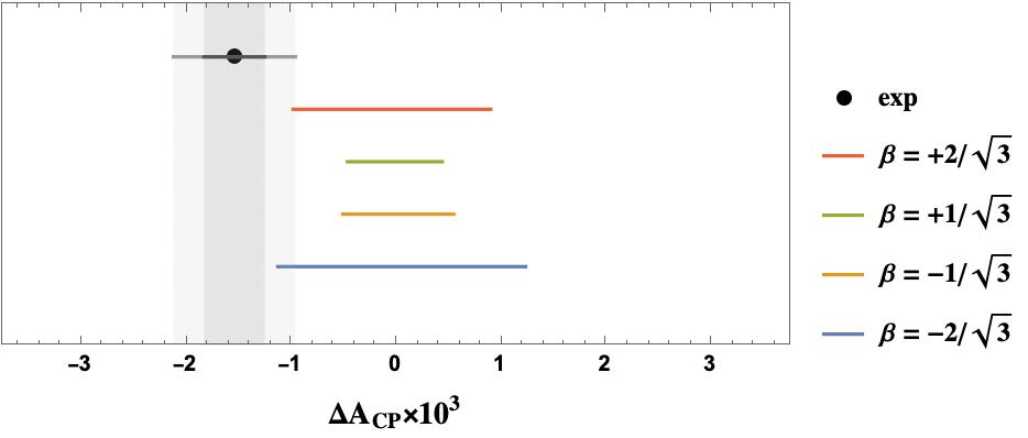
Large values of correspond to large values of the hadronic matrix elements, a statement that can be made more precise if the difference is considered, as in Fig. 6. When the ratios are varied in the ranges quoted above, for the variants with it is possible to find a set of parameters (the 331 parameters plus ratios of hadronic matrix elements) giving in agreement with data. For larger values of the also for can be obtained. An insight into the required size of the ratios of the hadronic matrix elements can be gained considering for which, as shown in Fig. 6, the 331 result for has an overlap with the experimental range. The largest value of is obtained in correspondence of the ratios :
| (87) |
and of the ratios :
| (88) |
The conclusion is that large individual CP asymmetries and can be obtained provided that two conditions are verified: the phases are in the ranges obtained in 331 models and the ratios of the hadronic matrix elements are large, close to the values in (87) and (88). This last condition can be verified by future explicit calculations, namely using lattice QCD.
4.3 , correlations with and observables
We shall next investigate correlations of charm observables with those in the and systems, a striking possibility within the 331 models.
In Fig. 7 we show the correlation between the asymmetry in (37) and the mixing-induced CP asymmetries and in the and systems. The message from these plots is clear. CP violation in the charm system is by orders of magnitude smaller than in the and systems. Even in the system is roughly by two orders of magnitude smaller than .

In Fig. 8 we show the correlation between and in 331 for the four variants with considered in this paper and TeV. The SM contribution is set to zero in both observables. We note that can reach values of order , that is by roughly six orders of magnitude larger than the result (74) obtained within the SM but still much smaller than the experimental bound.
It is worth considering the impact on these results of the measurement
| (89) |
where is the average time integrated branching ratio [61]:
| (90) |
with and [52]. is analogous to in Eq. (31) for , is the mean lifetime and the width difference of the heavy and light mass eigenstates. In Fig. 8, imposing that lies in the experimental range in Eq. (89) within we find the blue regions which show that this constraint allows only for values of below . The reason for this further suppression is evident from Fig. 9 where we show the correlation between and in 331 models with parameters as in Fig.8. Indeed, to suppress the SM branching ratio for to achieve a better agreement with the experimental measurement (89), a smaller is implied. This would not be the case if the data for was above the SM expectation.
In Figs. 10 and 11 we show the correlations of with the branching ratios for and , respectively. We observe that the largest values of are found for the smallest 331 contributions to both kaon decays. The largest contributions to these decays in 331 models amount to roughly of the SM value and these modest effects could be tested one day, in particular if the future data turned out to depart significantly from the SM predictions within the SM central value represented by black dots in these figures.
The pattern turns out to be different in Figs. 12 and 13, where we show the correlations of with branching ratios for and , respectively. Without the constraint the largest 331 contributions to and are accompanied by largest contributions to . This is in particular seen in the case of in Fig. 12. However, when the data on are imposed, 331 effects in are dwarfed as already seen in Fig. 9.


5 Conclusions
We have performed a detailed analysis of FCNC processes in the charm sector in the context four variants of 331 models. The motivation for this analysis arose from the observation [5] that in the case of contributions there are no new free parameters beyond those present already in the and meson systems. As a result definite ranges for NP effects in various charm observables could be obtained.
In the SM FCNC in the charm system are very strongly GIM suppressed so that a contribution of that appears already at tree-level could in principle imply NP effects in the charm sector by orders of magnitude larger than it is possible within the SM. In fact if we performed our analysis first for the charm system, ignoring correlations with and meson systems, very large effects would be possible. However, as our analysis demonstrates most of these effects would be subsequently dwarfed by imposing the contraints from and meson systems that were analyzed in the past [8, 9, 10, 11, 12].
In particular we find very small effects in mixing although the effects are still larger than short-distance contributions within the SM.
Our results are presented in the plots in Section 4 and in the accompanying comments. Here we list the most remarkable results.
- •
As seen in Fig. 3 the semileptonic asymmetry can be as large as and therefore much larger than in the SM.
- •
As seen in Fig. 9, the correlation between and implies the suppression of the latter branching ratio if a better agreement with the experimental data for is to be achieved. Yet, despite this suppression the branching ratio can reach values of a few which is by six orders larger than its SM value.
- •
The correlations between and the branching ratios for , and show patterns that depend on the specific 331 model considered. However, if future data on theoretically clean decays and and also short distance part in will show deviations from SM expectations by more than the 331 models will not be able to explain them.
- •
We are looking forward to the improved experimental data on all observables discussed by us to see whether 331 models will survive these tests.
Acknowledgements
We thank S. Fajfer and S. Schacht for discussions. This study has been carried out within the INFN project (Iniziativa Specifica) QFT-HEP. A.J.B acknowledges financial support from the Excellence Cluster ORIGINS, funded by the Deutsche Forschungsgemeinschaft (DFG, German Research Foundation) under Germany´s Excellence Strategy – EXC-2094 – 390783311.


Appendix A effective Hamiltonian and RG evolution of the coefficients
The most general effective Hamiltonian governing the decays , can be written as
| (91) | |||||
where , , and . The operators are classified according to the standard nomenclature:
- •
current-current operators:
(92) - •
QCD penguins
(93) (94) - •
QED penguins
(95) (96) - •
chromomagnetic operator
(97) - •
scalar and tensor operators
(98) (99)
The operators are obtained exchanging . In the SM only is present at tree level; the operators , the QCD penguins and are generated at ; the QED penguins are negligible because of their small coefficients, and the scalar and tensor operators are absent. In 331 models, at the scale the tree-level exchange produces the operators and . When evolved at the low scale other operators are generated. Neglecting the scalar and tensor operators (absent in SM and in 331 model), the RG evolution can be done separately for the 10 operators in Eqs. (92), (93)-(94), (95)-(96) and for . The anomalous dimension matrix (ADM) for the set of 10 operators is:
| (100) |
where is the number of colors, , and are the number of active quark flavors, active up- and active down-type quarks, respectively. For the chromomagnetic operator , the LO anomalous dimension reads
| (101) |
The result of the evolution of the 331 operators leads to the generation of the operators having the structure of , with coefficients given by:
| (102) | |||||
| (103) | |||||
| (104) | |||||
| (105) | |||||
| (106) | |||||
| (107) |
References
- [1] G. Wilkinson, Charming synergies: the role of charm-threshold studies in the search for physics beyond the Standard Model, arXiv:2107.08414.
- [2] A. Lenz and G. Wilkinson, Mixing and violation in the charm system, arXiv:2011.04443.
- [3] W. Altmannshofer and P. Stangl, New Physics in Rare B Decays after Moriond 2021, arXiv:2103.13370.
- [4] M. Algueró, B. Capdevila, S. Descotes-Genon, J. Matias, and M. Novoa-Brunet, global fits after Moriond 2021 results, in 55th Rencontres de Moriond on QCD and High Energy Interactions, 4, 2021. arXiv:2104.08921.
- [5] P. Colangelo, F. De Fazio, and F. Loparco, transitions of mesons: 331 model facing Standard Model null tests, arXiv:2107.07291.
- [6] F. Pisano and V. Pleitez, An model for electroweak interactions, Phys. Rev. D 46 (1992) 410–417, [hep-ph/9206242].
- [7] P. H. Frampton, Chiral dilepton model and the flavor question, Phys. Rev. Lett. 69 (1992) 2889–2891.
- [8] A. J. Buras, F. De Fazio, J. Girrbach, and M. V. Carlucci, The Anatomy of Quark Flavour Observables in 331 Models in the Flavour Precision Era, JHEP 02 (2013) 023, [arXiv:1211.1237].
- [9] A. J. Buras, F. De Fazio, and J. Girrbach, 331 models facing new data, JHEP 02 (2014) 112, [arXiv:1311.6729].
- [10] A. J. Buras, F. De Fazio, and J. Girrbach-Noe, - mixing and -mediated FCNCs in models, JHEP 08 (2014) 039, [arXiv:1405.3850].
- [11] A. J. Buras and F. De Fazio, in 331 Models, JHEP 03 (2016) 010, [arXiv:1512.02869].
- [12] A. J. Buras and F. De Fazio, 331 Models Facing the Tensions in Processes with the Impact on , and , JHEP 08 (2016) 115, [arXiv:1604.02344].
- [13] J. M. Cabarcas, D. Gomez Dumm, and R. Martinez, Flavor changing neutral currents in 331 models, J. Phys. G 37 (2010) 045001, [arXiv:0910.5700].
- [14] A. C. B. Machado, J. C. Montero, and V. Pleitez, Flavor-changing neutral currents in the minimal 3-3-1 model revisited, Phys. Rev. D 88 (2013), no. 11 113002, [arXiv:1305.1921].
- [15] D. Cogollo, A. V. de Andrade, F. S. Queiroz, and P. Rebello Teles, Novel sources of Flavor Changed Neutral Currents in the model, Eur. Phys. J. C 72 (2012) 2029, [arXiv:1201.1268].
- [16] HFLAV Collaboration, Y. S. Amhis et al., Averages of b-hadron, c-hadron, and -lepton properties as of 2018, Eur. Phys. J. C 81 (2021), no. 3 226, [arXiv:1909.12524].
- [17] LHCb Collaboration, R. Aaij et al., Observation of the mass difference between neutral charm-meson eigenstates, arXiv:2106.03744.
- [18] V. Bhardwaj, M. Dorigo, and F.-S. Yu, Summary of WG7 at CKM 2018: ”Mixing and violation in the system: , , , , and direct violation in decays”, 2019. arXiv:1901.08131.
- [19] A. Cerri, V. V. Gligorov, S. Malvezzi, J. Martin Camalich, and J. Zupan, Opportunities in Flavour Physics at the HL-LHC and HE-LHC, arXiv:1812.07638.
- [20] F. Gabbiani, E. Gabrielli, A. Masiero, and L. Silvestrini, A Complete analysis of FCNC and CP constraints in general SUSY extensions of the standard model, Nucl. Phys. B477 (1996) 321–352, [hep-ph/9604387].
- [21] UTfit Collaboration, M. Bona et al., Model-independent constraints on operators and the scale of new physics, JHEP 0803 (2008) 049, [arXiv:0707.0636]. Updates available on http://www.utfit.org.
- [22] G. Isidori, Y. Nir, and G. Perez, Flavor Physics Constraints for Physics Beyond the Standard Model, Ann.Rev.Nucl.Part.Sci. 60 (2010) 355, [arXiv:1002.0900].
- [23] J. Charles, S. Descotes-Genon, Z. Ligeti, S. Monteil, M. Papucci, et al., Future sensitivity to new physics in , and mixings, Phys. Rev. D89 (2014) 033016, [arXiv:1309.2293].
- [24] E. Golowich, J. Hewett, S. Pakvasa, and A. A. Petrov, Implications of - Mixing for New Physics, Phys. Rev. D 76 (2007) 095009, [arXiv:0705.3650].
- [25] E. Golowich, J. Hewett, S. Pakvasa, and A. A. Petrov, Relating Mixing and with New Physics, Phys. Rev. D 79 (2009) 114030, [arXiv:0903.2830].
- [26] A. J. Buras, M. Misiak, and J. Urban, Two loop QCD anomalous dimensions of flavor changing four quark operators within and beyond the standard model, Nucl. Phys. B 586 (2000) 397–426, [hep-ph/0005183].
- [27] I. I. Bigi, M. Blanke, A. J. Buras, and S. Recksiegel, CP Violation in Oscillations: General Considerations and Applications to the Littlest Higgs Model with T-Parity, JHEP 07 (2009) 097, [arXiv:0904.1545].
- [28] Y. Grossman, Y. Nir, and G. Perez, Testing New Indirect CP Violation, Phys. Rev. Lett. 103 (2009) 071602, [arXiv:0904.0305].
- [29] LHCb Collaboration, R. Aaij et al., Observation of CP Violation in Charm Decays, Phys. Rev. Lett. 122 (2019), no. 21 211803, [arXiv:1903.08726].
- [30] M. Golden and B. Grinstein, Enhanced CP Violations in Hadronic Charm Decays, Phys. Lett. B 222 (1989) 501–506.
- [31] Y. Grossman, A. L. Kagan, and Y. Nir, New physics and CP violation in singly Cabibbo suppressed D decays, Phys. Rev. D 75 (2007) 036008, [hep-ph/0609178].
- [32] J. Brod, A. L. Kagan, and J. Zupan, Size of direct CP violation in singly Cabibbo-suppressed D decays, Phys. Rev. D 86 (2012) 014023, [arXiv:1111.5000].
- [33] D. Pirtskhalava and P. Uttayarat, CP Violation and Flavor SU(3) Breaking in D-meson Decays, Phys. Lett. B 712 (2012) 81–86, [arXiv:1112.5451].
- [34] B. Bhattacharya, M. Gronau, and J. L. Rosner, CP asymmetries in singly-Cabibbo-suppressed decays to two pseudoscalar mesons, Phys. Rev. D 85 (2012) 054014, [arXiv:1201.2351].
- [35] T. Feldmann, S. Nandi, and A. Soni, Repercussions of Flavour Symmetry Breaking on CP Violation in D-Meson Decays, JHEP 06 (2012) 007, [arXiv:1202.3795].
- [36] H.-Y. Cheng and C.-W. Chiang, Direct CP violation in two-body hadronic charmed meson decays, Phys. Rev. D 85 (2012) 034036, [arXiv:1201.0785]. [Erratum: Phys.Rev.D 85, 079903 (2012)].
- [37] E. Franco, S. Mishima, and L. Silvestrini, The Standard Model confronts CP violation in and , JHEP 05 (2012) 140, [arXiv:1203.3131].
- [38] H.-Y. Cheng and C.-W. Chiang, symmetry breaking and CP violation in decays, Phys. Rev. D 86 (2012) 014014, [arXiv:1205.0580].
- [39] H.-Y. Cheng and C.-W. Chiang, Revisiting CP violation in and decays, Phys. Rev. D 100 (2019), no. 9 093002, [arXiv:1909.03063].
- [40] J. Brod, Y. Grossman, A. L. Kagan, and J. Zupan, A Consistent Picture for Large Penguins in , JHEP 10 (2012) 161, [arXiv:1203.6659].
- [41] G. Isidori, J. F. Kamenik, Z. Ligeti, and G. Perez, Implications of the LHCb Evidence for Charm CP Violation, Phys. Lett. B 711 (2012) 46–51, [arXiv:1111.4987].
- [42] G. F. Giudice, G. Isidori, and P. Paradisi, Direct CP violation in charm and flavor mixing beyond the SM, JHEP 04 (2012) 060, [arXiv:1201.6204].
- [43] W. Altmannshofer, R. Primulando, C.-T. Yu, and F. Yu, New Physics Models of Direct CP Violation in Charm Decays, JHEP 04 (2012) 049, [arXiv:1202.2866].
- [44] G. Hiller, Y. Hochberg, and Y. Nir, Supersymmetric , Phys. Rev. D 85 (2012) 116008, [arXiv:1204.1046].
- [45] M. Chala, A. Lenz, A. V. Rusov, and J. Scholtz, within the Standard Model and beyond, JHEP 07 (2019) 161, [arXiv:1903.10490].
- [46] H.-N. Li, C.-D. Lü, and F.-S. Yu, Implications on the first observation of charm CPV at LHCb, arXiv:1903.10638.
- [47] Y. Grossman and S. Schacht, The emergence of the rule in charm physics, JHEP 07 (2019) 020, [arXiv:1903.10952].
- [48] A. Dery and Y. Nir, Implications of the LHCb discovery of CP violation in charm decays, JHEP 12 (2019) 104, [arXiv:1909.11242].
- [49] A. Khodjamirian and A. A. Petrov, Direct CP asymmetry in and in QCD-based approach, Phys. Lett. B 774 (2017) 235–242, [arXiv:1706.07780].
- [50] S. Fajfer and N. Košnik, Prospects of discovering new physics in rare charm decays, Eur. Phys. J. C 75 (2015), no. 12 567, [arXiv:1510.00965].
- [51] A. Buras, Gauge Theory of Weak Decays. Cambridge University Press, 6, 2020.
- [52] Particle Data Group Collaboration, P. Zyla et al., Review of Particle Physics, PTEP 2020 (2020), no. 8 083C01.
- [53] G. Burdman, E. Golowich, J. L. Hewett, and S. Pakvasa, Rare charm decays in the standard model and beyond, Phys. Rev. D 66 (2002) 014009, [hep-ph/0112235].
- [54] Flavour Lattice Averaging Group Collaboration, S. Aoki et al., FLAG Review 2019: Flavour Lattice Averaging Group (FLAG), Eur. Phys. J. C 80 (2020), no. 2 113, [arXiv:1902.08191].
- [55] K. G. Chetyrkin, J. H. Kuhn, A. Maier, P. Maierhofer, P. Marquard, M. Steinhauser, and C. Sturm, Addendum to “Charm and bottom quark masses: An update”, arXiv:1710.04249. [Addendum: Phys.Rev.D 96, 116007 (2017)].
- [56] K. G. Chetyrkin, J. H. Kuhn, A. Maier, P. Maierhofer, P. Marquard, M. Steinhauser, and C. Sturm, Charm and Bottom Quark Masses: An Update, Phys. Rev. D 80 (2009) 074010, [arXiv:0907.2110].
- [57] A. J. Buras, M. Jamin, and P. H. Weisz, Leading and Next-to-leading QCD Corrections to Parameter and Mixing in the Presence of a Heavy Top Quark, Nucl. Phys. B 347 (1990) 491–536.
- [58] J. Urban, F. Krauss, U. Jentschura, and G. Soff, Next-to-leading order QCD corrections for the mixing with an extended Higgs sector, Nucl. Phys. B 523 (1998) 40–58, [hep-ph/9710245].
- [59] R. Gupta, T. Bhattacharya, and S. R. Sharpe, Matrix elements of four fermion operators with quenched Wilson fermions, Phys. Rev. D 55 (1997) 4036–4054, [hep-lat/9611023].
- [60] H.-W. Lin, S. Ohta, A. Soni, and N. Yamada, Charm as a domain wall fermion in quenched lattice QCD, Phys. Rev. D 74 (2006) 114506, [hep-lat/0607035].
- [61] K. De Bruyn, R. Fleischer, R. Knegjens, P. Koppenburg, M. Merk, A. Pellegrino, and N. Tuning, Probing New Physics via the Effective Lifetime, Phys. Rev. Lett. 109 (2012) 041801, [arXiv:1204.1737].