跳到论文正文
W Papers独立论文阅读器 arXiv:2107.10727 论文正文 计算阅读时间 · 0%
引用这篇论文根据当前论文元数据生成,正式投稿前建议核对。


License: arXiv.org perpetual non-exclusive license
arXiv:2107.10727v1 [quant-ph] 22 Jul 2021

Differential Equation Based Path Integral for System-Bath DynamicsThanks: Zhenning Cai’s work was supported by the Academic Research Fund of the Ministry of Education of Singapore under grant R-146-000-291-114.

Geshuo Wang Geshuo WangDepartment of Mathematics, National University of Singapore, Level 4, Block S17, 10 Lower Kent Ridge Road, Singapore 119076 Email address: geshuowang@u.nus.edu and Zhenning Cai Zhenning CaiDepartment of Mathematics, National University of Singapore, Level 4, Block S17, 10 Lower Kent Ridge Road, Singapore 119076 Email address: matcz@nus.edu.sg
Abstract.

We propose the differential equation based path integral (DEBPI) method to simulate the real-time evolution of open quantum systems. In this method, a system of partial differential equations is derived based on the continuation of a classical numerical method called iterative quasi-adiabatic propagator path integral (i-QuAPI). While the resulting system has infinite equations, we introduce a reasonable closure to obtain a series of finite systems. New numerical schemes can be derived by discretizing these differential equations. It is numerically verified that in certain cases, by selecting appropriate systems and applying suitable numerical schemes, the memory cost required in the i-QuAPI method can be significantly reduced.

Key words and phrases: 
Open quantum system, DEBPI, i-QuAPI

1. Introduction

In physics, an open quantum system refers to a quantum system coupled with an external environment (bath). In reality, no quantum system can be absolutely isolated, and therefore the study of open quantum system is of great importance and nowadays has wide applications in the fields including quantum optics [3], chemical physics [27, 9], quantum information [21] and even social sciences [8]. In general, for an open quantum system, the large number of degrees of freedom in the bath prevents us from directly computing the density matrix of the coupled system. To carry out simulations, the bath is usually assumed to be some analytically solvable models such as harmonic oscillators so that one can represent the quantum dynamics using path integrals, and the influence of the bath on the system of interest can be reduced to an influence functional [5].

Despite such simplification, the difficulty introduced by the system-bath coupling still exists because the influence functional couples the states of the system at any two time points, leading to a non-Markovian process. Such process is often formulated using an integro-differential equation (known as Nakajima-Zwanzig equation), where the effect of the bath is expressed as a memory kernel, represented by the Nakajima-Zwanzig operator [20, 30]. The numerical methods based on the computation of path integrals, such as quasi-adiabatic propagator path integral (QuAPI) [12] and hierarchical equations of motion (HEOM) [25, 24] methods, require significant memory cost to store the contributions from different paths. To reduce the storage requirement, one idea is to make use of the decaying property of the influence functional to develop iterative schemes. One typical method is the iterative QuAPI (i-QuAPI) method [13, 14], which truncates the influence functional to achieve finite memory length, so that partial summation can be carried out in the path integral. Other approaches based on this idea include the blip-summed method [16, 17], small matrix decomposition of the path integral (SMatPI) method [18], and important path sampling [23] design algorithms, which explore extra the numerical sparsity of the problem to further reduce the memory cost. Some stochastic methods, such as diagrammatic quantum Monte Carlo (dQMC) method [28] and inchworm Monte Carlo method [4, 1, 29, 2], apply stochastic approaches to estimate path integrals. These methods no longer suffer from the curse of memory cost. However, numerical sign problem may appear for long-time simulations [11, 2]. There are also some modeling techniques to simplify the Nakajima-Zwanzig equation, among which the Lindblad equation [10, 6] considers the weak coupling limit, so that the memory effect can be ignored and the master equation becomes Markovian. Other approaches based on computable master equations include the post-Markovian master equation [22] and the generalized quantum master equation [7].

Despite the fast progress in the numerical computation of open quantum systems, the i-QuAPI method remains as one of the fundamental and reliable methods, and is often used to compute reference solutions in the development of other methods. Since the strongest limitation of i-QuAPI is its memory cost, which grows exponentially with 1/Δ​t1/\Delta t, the present paper follows the basic idea of the i-QuAPI method and tries to break such exponential relationship by developing the differential equation based path integral (DEBPI) method. The DEBPI method formulates a system of differential equations such that i-QuAPI can be considered as its numerical scheme. Afterwards, we can re-design the numerical scheme by discretizing the PDE system. It is numerically verified that in certain cases, the memory cost can be significantly reduced.

Throughout this paper, we will mainly focus on a simple open quantum system consisting of a flipping spin and a thermal bath. Despite the simple setting of the system, it contains all the difficulties related to the system-bath coupling in general open quantum systems. We refer the authors to [26] for some detailed discussion on this model.

For the rest of this paper, we present the derivation of DEBPI method and some numerical tests. Section 2 is a brief introduction to the spin-boson model and the i-QuAPI method. In order to derive the continuous formulation for i-QuAPI method, we give a representation of the continuation of path segments and introduce notations for the relative quantities in Section 3. With all the preparation in Sections 2 and 3, we derive a governing partial differential equation system and discuss the required boundary condition in Section 4. In addition, as the partial differential equation system includes infinite equations, we also provide the idea of dimensional truncation and the closure of the system in Section 4. In Section 5, we carry out some numerical experiments based on finite difference discretization method for DEBPI method and compare our results with i-QuAPI method. In Section 6, we outline the application of the idea in other finite state models and give a simple conclusion. The derivation of i-QuAPI method is given in the appendix for reference.

2. Spin-boson model and iterative QuAPI method

In a quantum system with Hamiltonian HH, the density matrix ρ⁡(t)\rho(t) satisfies the von Neumann equation

i​ℏ​dd​t​ρ​(t)=H​ρ​(t)−ρ⁡(t)​H,\mathrm{i}\hbar\frac{\mathrm{d}}{\mathrm{d}t}\rho(t)=H\rho(t)-\rho(t)H,

where i\mathrm{i} is the imaginary unit, and ℏ\hbar is the reduced Planck’s constant. For simplicity, ℏ\hbar is set to be 1 in this paper. The solution to the von Neumann equation can be formally written as ρ⁡(t)=e−i​H​t​ρ​(0)​ei​H​t\rho(t)=\mathrm{e}^{-\mathrm{i}Ht}\rho(0)\mathrm{e}^{\mathrm{i}Ht}.

For an open quantum system, the operators are defined on the tensor product space ℋs⊗ℋb\mathcal{H}_{s}\otimes\mathcal{H}_{b}, where ℋs\mathcal{H}_{s} and ℋb\mathcal{H}_{b} represent the Hilbert spaces for the system and the bath, respectively. In general, the Hamiltonian HH has the form

(1) H=Hs⊗idb+ids⊗Hb+Hs​bH=H_{s}\otimes\mathrm{id}_{b}+\mathrm{id}_{s}\otimes H_{b}+H_{sb}

where ids,idb\mathrm{id}_{s},\mathrm{id}_{b} are the identity operators on ℋs\mathcal{H}_{s} and ℋb\mathcal{H}_{b}, respectively. The operators HsH_{s} and HbH_{b} are the Hamiltonian operators for the system and the bath without coupling, and the last term Hs​bH_{sb} describes the system-bath interaction, which lead to entanglement between system and bath. For simplicity, below we focus on the study of a specific case of the open quantum system, where the system contains a single spin. The model and the iterative QuAPI method will be introduced in the following subsections.

2.1. Spin-boson model

A fundamental example of open quantum systems is the spin-boson model where the Hilbert spaces are

ℋs=span⁡{|−1⟩,|+1⟩},ℋb=⨂j(L2​(ℝ3))\mathcal{H}_{s}=\SPAN\{\ket{-1},\ket{+1}\},\quad\mathcal{H}_{b}=\bigotimes_{j}(L^{2}(\mathbb{R}^{3}))

with L2​(ℝ3)L^{2}(\mathbb{R}^{3}) being the L2L^{2} space over ℝ3\mathbb{R}^{3} and jj is the index of harmonic oscillators. In spin-boson system, there are two energy levels in the energy set 𝒮={−1,+1}\mathcal{S}=\{-1,+1\}. In such a system, the Hamiltonians in (1) can be represented by

(2) Hs=ϵ​σ^z+Δ​σ^x,Hb=∑j12​(p^j2+ωj2​q^j2),Hs​b=σ^z⊗(∑jcj​q^j)H_{s}=\epsilon\hat{\sigma}_{z}+\Delta\hat{\sigma}_{x},\quad H_{b}=\sum_{j}\frac{1}{2}(\hat{p}_{j}^{2}+\omega_{j}^{2}\hat{q}_{j}^{2}),\quad H_{sb}=\hat{\sigma}_{z}\otimes\left(\sum_{j}c_{j}\hat{q}_{j}\right)

where σ^x,σ^z\hat{\sigma}_{x},\hat{\sigma}_{z} are Pauli matrices, and p^j\hat{p}_{j} and q^j\hat{q}_{j} are momentum operator and position operator of the jj-th harmonic oscillator, respectively. ϵ\epsilon represents the energy difference between two spin states and Δ\Delta is the frequency of the spin flipping. The parameter ωj\omega_{j} is the frequency of the jj-th harmonic oscillator while cjc_{j} is the coupling intensity between the spin and the jj-th harmonic oscillator.

For convenience, it is supposed that the system and bath are not coupled initially, which can be expressed mathematically by

ρ⁡(0)=ρs​(0)⊗ρb​(0)\rho(0)=\rho_{s}(0)\otimes\rho_{b}(0)

with ρs\rho_{s} and ρb\rho_{b} representing the density matrices of the system and the bath, respectively. The reduced density matrix, which is the density matrix of the system, can be represented by the partial trace of the whole density matrix:

ρs​(t)=trb⁡ρ⁡(t),\rho_{s}(t)=\tr_{b}\rho(t),

where trb\tr_{b} is the partial trace operator with respect to ℋb\mathcal{H}_{b}. In the spin-boson model, this reduced density matrix ρs\rho_{s} is essentially a 2×22\times 2 matrix. The algorithm discussed in this paper can be generalized to more complicated model. However, in this paper, only spin-boson model is involved and there is a simple discussion about other finite state models in Section 6.

2.2. Iterative QuAPI method

To compute the reduced density matrix in a spin-boson model, the iterative quasi-adiabatic propagator path integral (i-QuAPI) method is developed in [13, 14]. It is assumed that the density matrix has a finite memory length TT although it is non-Markovian. Then we choose the time step Δ​t\Delta t such that Δ​k:=T/Δ​t\Delta k:=T/\Delta t is an integer. The density matrix can be obtained through computing the maps Al:𝒮2​Δ​k→ℂA_{l}:\mathcal{S}^{2\Delta k}\rightarrow\mathbb{C} iteratively:

(3) A0​(SΔ​k−1,⋯,S0):=∏k1=0Δ​k−1∏k2=0k1I⁡(Sk1,Sk2)​⟨s0+|ρs​(0)|s0−⟩;\displaystyle A_{0}(S_{\Delta k-1},\cdots,S_{0}):=\prod_{k_{1}=0}^{\Delta k-1}\prod_{k_{2}=0}^{k_{1}}I(S_{k_{1}},S_{k_{2}})\matrixelement{s_0^+}{\rho_s(0)}{s_0^-};
(4) Λ⁡(Sk,⋯,Sk−Δ​k):=∏m=0Δ​kI⁡(Sk,Sk−m);\displaystyle\Lambda(S_{k},\cdots,S_{k-\Delta k}):=\prod_{m=0}^{\Delta k}I(S_{k},S_{k-m});
(5) Ak−Δ​k+1​(Sk,⋯,Sk−Δ​k+1):=∑Sk−Δ​k∈𝒮2Λ⁡(Sk,⋯,Sk−Δ​k)​Ak−Δ​k​(Sk−1,⋯,Sk−Δ​k)\displaystyle A_{k-\Delta k+1}(S_{k},\cdots,S_{k-\Delta k+1}):=\sum_{S_{k-\Delta k}\in\mathcal{S}^{2}}\Lambda(S_{k},\cdots,S_{k-\Delta k})A_{k-\Delta k}(S_{k-1},\cdots,S_{k-\Delta k})
for ​k=Δ​k,⋯,N−1.\displaystyle\qquad\text{for }k=\Delta k,\cdots,N-1.

where Sj=(sj+,sj−)S_{j}=(s_{j}^{+},s_{j}^{-}) represents the states on both branches of the path and I⁡(Sj,Sj′)I(S_{j},S_{j^{\prime}}) is defined to be

(6) I⁡(Sj,Sj′)={e−(sj+−sj−)​(ηj,j′​sj′+−ηj,j′∗​sj′−),j−j′≠1⟨sj+|e−i​H0​Δ​t|sj−1+⟩​⟨sj−1−|ei​H0​Δ​t|sj−⟩​e−(sj+−sj−)​(ηj,j′​sj′+−ηj,j′∗​sj′−),j−j′=1I(S_{j},S_{j^{\prime}})=\begin{cases}\mathrm{e}^{-(s_{j}^{+}-s_{j}^{-})(\eta_{j,j^{\prime}}s_{j^{\prime}}^{+}-\eta_{j,j^{\prime}}^{*}s_{j^{\prime}}^{-})},\quad j-j^{\prime}\not=1\\ \matrixelement{s_j^+}{\e^{-\ii H_0 \dt}}{s_{j-1}^+}\matrixelement{s_{j-1}^-}{\e^{\ii H_0 \dt}}{s_j^-}\mathrm{e}^{-(s_{j}^{+}-s_{j}^{-})(\eta_{j,j^{\prime}}s_{j^{\prime}}^{+}-\eta_{j,j^{\prime}}^{*}s_{j^{\prime}}^{-})},\quad j-j^{\prime}=1\end{cases}

where η∗\eta^{*} is the complex conjugate of η\eta. The complex function η\eta has different forms for different jj and j′j^{\prime} [19]. For example, if only positive frequencies are considered, when 0<j′<j<N0<j^{\prime}<j<N,

(7) ηj,j′=4π​∫0∞d​ω​J⁡(ω)ω2​sin2⁡(ω​Δ​t2)​(coth⁡(β​ω2)​cos⁡(ω​Δ​t​(k−k′))−i​sin⁡(ω​Δ​t​(k−k′))).\eta_{j,j^{\prime}}=\frac{4}{\pi}\int_{0}^{\infty}\mathrm{d}\omega\frac{J(\omega)}{\omega^{2}}\sin^{2}\left(\frac{\omega\Delta t}{2}\right)\left(\coth\left(\frac{\beta\omega}{2}\right)\cos(\omega\dt(k-k'))-\mathrm{i}\sin(\omega\dt(k-k'))\right).

In the expression of η\eta,

J⁡(ω)=π2​∑jcj2mj​ωj​δ​(ω−ωj)J(\omega)=\frac{\pi}{2}\sum_{j}\frac{c_{j}^{2}}{m_{j}\omega_{j}}\delta(\omega-\omega_{j})

and δ\delta is the Dirac delta function. The derivation of the i-QuAPI method can be found in the appendix. With the values of Ak−Δ​k​(Sk,⋯,Sk−Δ​k)A_{k-\Delta k}(S_{k},\cdots,S_{k-\Delta k}), the entries in the reduced density matrix can be computed by

(8) ρs​(N​Δ​t)=∑SN−Δ​k+1,⋯,SN∈𝒮AN−Δ​k​(SN,⋯,SN−Δ​k+1)​|sN+⟩​⟨sN−|.\rho_{s}(N\Delta t)=\sum_{S_{N-\Delta k+1},\cdots,S_{N}\in\mathcal{S}}A_{N-\Delta k}(S_{N},\cdots,S_{N-\Delta k+1})\ket{s_N^+}\bra{s_N^-}.

The system-bath coupling leads to a non-Markovian process where the evolution of the system density matrix depends on the complete history, and the intensity of the dependence is determined by the discrete bath response function ηj,j′\eta_{j,j^{\prime}}. The method of iterative quasi-adiabatic propagator path integral (i-QuAPI), however, makes use of the decaying property of the discrete bath response function ηj,j′\eta_{j,j^{\prime}} and truncate the memory length to a fixed and finite time TT, so that the evolution is similar to the time-delay systems, making the simulation more feasible.

The major obstacle of this method is the memory constraint. In each step, there are in total 22​Δ​k2^{2\Delta k} different values of AlA_{l} to be stored in the memory. As Δ​k\Delta k is defined to be T/Δ​tT/\Delta t, and TT is fixed according to the problem itself, the restriction on Δ​k\Delta k directly results in a lower bound of Δ​t\Delta t. The contradiction is that for more accurate results, smaller Δ​t\Delta t should be chosen, which is prohibited by the memory. For example, if the truncation time TT is 1.5 and the time step Δ​t\Delta t is chosen to be 0.10.1, then Δ​k=15\Delta k=15 and the memory cost is approximately 22×15×(16​ bytes)=16​GB2^{2\times 15}\times(16\text{ bytes})=16\text{GB}, where “16 bytes” stands for the size of a double-precision complex number. However, if a smaller time step, for example, Δ​t=0.075\Delta t=0.075, is required, the memory cost will become 22×20×(16​ bytes)=16​TB2^{2\times 20}\times(16\text{ bytes})=16\text{TB}, which is beyond the capacity of most workstations.

3. Continuation of the Path Segments

In order to cut off the memory cost, the most straightforward idea is to reduce the number of path segments that need to be stored. Equation (6) shows that when the flipping rate Δ\Delta is small, the path segments with many spin flips may have little contribution to the density matrix, and therefore may be dropped in the path integrals without much loss of numerical accuracy. To achieve this, we will carry out the following:

  1. (1)

    Find the governing equations of i-QuAPI by taking the limit Δ​t→0\Delta t\rightarrow 0;

  2. (2)

    Truncate the small terms and provide a reasonable closure;

  3. (3)

    Discretize the resulting system partial differential equations to get a scheme with less memory cost.

In this section, we will focus only on the representation of the unknown function which stands for a path segment with memory time TT. The complete form of the governing equations will be derived in Section 4.

3.1. Representation of the paths

In the i-QuAPI method, each AlA_{l} has a set of parameters Sk−1,⋯,Sk−Δ​kS_{k-1},\cdots,S_{k-\Delta k}, representing a path segment in the path integral. While the sequence Sk−1,⋯,Sk−Δ​kS_{k-1},\cdots,S_{k-\Delta k} represents the discrete path segment, we can regard it as a piecewise constant path segment of the continuous time sΔ​t:[0,T)→𝒮2s_{\Delta t}:[0,T)\rightarrow\mathcal{S}^{2}, defined by

(9) sΔ​t(τ)=Sk−j,∀τ∈[(Δk−j)Δt,(Δk−j+1)Δt),j=1,⋯,Δk,s_{\Delta t}(\tau)=S_{k-j},\quad\forall\tau\in\Big[(\Delta k-j)\Delta t,~~(\Delta k-j+1)\Delta t\Big),\quad j=1,\cdots,\Delta k,

where Δ​t=T/Δ​k\Delta t=T/\Delta k. More generally, we would like to consider any path segment h:[0,T)→𝒮2h:[0,T)\rightarrow\mathcal{S}^{2} with finite discontinuities, where each discontinuity denotes a flip of the classical spin. We assume that there are DD spin flips in the path segment hh. To define hh, we introduce a DD-dimensional open simplex △t(D)\triangle_{t}^{(D)}:

(10) △t(D)={(τ1,⋯,τD)|τ1>0,⋯,τD>0;∑k=1Dτk<t}\triangle_{t}^{(D)}=\left\{(\tau_{1},\cdots,\tau_{D})\,\bigg|\,\tau_{1}>0,\cdots,\tau_{D}>0;~~\sum_{k=1}^{D}\tau_{k}<t\right\}

so that hh has the form

(11) h⁡(τ)={(r0+,r0−),if ​τ∈[0,τ1),(rd+,rd−),if τ∈[∑k=1dτk,∑k=1d+1τk),d=1,⋯,D−1,(rD+,rD−),if ​τ∈[∑k=1Dτk,T),h(\tau)=\left\{\begin{array}[]{ll}(r_{0}^{+},r_{0}^{-}),&\text{if }\tau\in[0,\tau_{1}),\\ (r_{d}^{+},r_{d}^{-}),&\text{if }\tau\in\left[\sum_{k=1}^{d}\tau_{k},\sum_{k=1}^{d+1}\tau_{k}\right),\quad d=1,\cdots,D-1,\\ (r_{D}^{+},r_{D}^{-}),&\text{if }\tau\in\left[\sum_{k=1}^{D}\tau_{k},T\right),\end{array}\right.

where (τ1,⋯,τD)∈△T(D)(\tau_{1},\cdots,\tau_{D})\in\triangle^{(D)}_{T}. In hh, we allow the locations of the jumps to be anywhere in (0,T)(0,T) instead of only being the multiples of Δ​t\Delta t. For the paths sΔ​ts_{\Delta t} and hh, we use sΔ​t+s_{\Delta t}^{+} (sΔ​t−s_{\Delta t}^{-}) and h+h^{+} (h−h^{-}) to denote their positive (negative) branches.

With these definitions, it is natural to express the quantity Ak−Δ​k​(Sk−1,⋯,Sk−Δ​k)A_{k-\Delta k}(S_{k-1},\cdots,S_{k-\Delta k}) as A⁡((k−Δ​k)​Δ​t,sΔ​t)A((k-\Delta k)\Delta t,s_{\Delta t}), where the first argument (k−Δ​k)​Δ​t(k-\Delta k)\Delta t plays the role of the subscript (k−Δ​k)(k-\Delta k), denoting the starting time of the path segment. This can then be further extended to continuous time by writing the quantity as A⁡(t,h)A(t,h) for any t⩾0t\geqslant 0 and hh holding the form (11). However, such a quantity A⁡(t,h)A(t,h) includes a non-classical argument hh, which is inconvenient for the formulation of differential equations and the design of numerical scheme. We would therefore like to find a more explicit form of A⁡(t,h)A(t,h) containing only real parameters. With the assumption that hh contains only finite discontinuities, the path segment can be fully determined by the following set of parameters:

  • •

    (r+,r−)(r^{+},r^{-}): the state of the path at time tt, i.e. the value of h⁡(0)=(h+​(0),h−​(0))=(r0+,r0−)h(0)=(h^{+}(0),h^{-}(0))=(r_{0}^{+},r_{0}^{-}).

  • •

    DD: the number of spin flips (discontinuous points) in hh.

  • •

    sgn\mathrm{sgn}: a list of DD signs representing the branch of each spin flip. Each sign is either “++” (representing the positive branch h+h^{+}) or “−-” (representing the negative branch h−h^{-}). In addition, we introduce an augmenting operation by adding a sign at the beginning of sgn\mathrm{sgn}. For example, if sgn=[+,−,+,+]\mathrm{sgn}=[+,-,+,+], then [+,sgn]:=[+,+,−,+,+][+,\mathrm{sgn}]:=[+,+,-,+,+].

  • •

    (τ1,⋯,τD)∈△(D)(\tau_{1},\cdots,\tau_{D})\in\triangle^{(D)}: a sequence of times with the following meaning:

    τk={time difference of the first spin flip and the starting time t, if ​k=1;time difference of the k-th flip and the (k−1)-th flip, if ​k=2,⋯,D.\tau_{k}=\begin{cases}\text{time difference of the first spin flip and the starting time $t$},\text{ if }k=1;\\ \text{time difference of the $k$-th flip and the $(k-1)$-th flip},\text{ if }k=2,\cdots,D.\end{cases}

For example, suppose the truncation time is T=4T=4 and the graph of the path segment hh is given in Figure 1. Then the corresponding parameters are

  • •

    (r+,r−)=(h+​(0),h−​(0))=(+1,−1)(r^{+},r^{-})=(h^{+}(0),h^{-}(0))=(+1,-1);

  • •

    D=5D=5 (total number of spin flips, 2 in positive branch and 3 in negative branch);

  • •

    sgn=[+,−,−,+,−]\mathrm{sgn}=[+,-,-,+,-] (branches of the spin flips);

  • •

    [τ1,τ2,τ3,τ4,τ5]=[1.0,0.5,0.5,0.5,1.0][\tau_{1},\tau_{2},\tau_{3},\tau_{4},\tau_{5}]=[1.0,0.5,0.5,0.5,1.0] (indicating the times of the spin flips are 1.01.0, 1.51.5, 2.02.0, 2.52.5, 3.53.5 from tt).

012.5T=4T=4tt+1-1h+h^{+}01.523.5T=4T=4tt-1+1h−h^{-}
Figure 1. An example of function hh.

Based on such notations, we write down the continuous version of AlA_{l} as

(12) A(r+,r−)D,sgn​(t,[τ1,⋯,τD]).A_{(r^{+},r^{-})}^{D,\mathrm{sgn}}(t,[\tau_{1},\cdots,\tau_{D}]).

In the example given in Figure 1, AA can be written as

(13) A(+1,−1)5,[+,−,−,+,−]​(t,[1.0,0.5,0.5,0.5,1.0]).A_{(+1,-1)}^{5,[+,-,-,+,-]}(t,[1.0,0.5,0.5,0.5,1.0]).

An advantage of the notation (12) is that we can define the value of (12) for (τ1,⋯,τD)∈∂△T(D)(\tau_{1},\cdots,\tau_{D})\in\partial\triangle_{T}^{(D)} by taking the limit. In other words, the domain of definition for (τ1,⋯,τD)(\tau_{1},\cdots,\tau_{D}) can be extended from △T(D)\triangle_{T}^{(D)} to △T(D)¯\overline{\triangle_{T}^{(D)}}, which is important for us to close the system and formulate the boundary conditions in future sections. Note that when (τ1,⋯,τD)(\tau_{1},\cdots,\tau_{D}) takes values on ∂△T(D)\partial\triangle_{T}^{(D)}, the path segment hh may have one or more spin flips at the same time, or have spin flips at the initial time or the final time. Nevertheless, both notations A⁡(t,h)A(t,h) and (12) will be used in our further discussions according to the context. The precise relation between A⁡(t,h)A(t,h) and Ak−Δ​kA_{k-\Delta k} will be detailed later in Section 3.3.

In i-QuAPI, another quantity Λ⁡(Sk,⋯,Sk−Δ​k)\Lambda(S_{k},\cdots,S_{k-\Delta k}) is also determined by a path segment, while it has one more argument than Ak−Δ​k​(Sk−1,⋯,Sk−Δ​k)A_{k-\Delta k}(S_{k-1},\cdots,S_{k-\Delta k}). In the continuous form, the length of this extra argument becomes infinitesimal so that the associated continuous quantity is also expected to be determined by hh. This will be discussed in detail in Section 3.2. The integral over the paths, which forms the density matrix, will be considered in Section 3.4.

In the following sections, our major task is to take the continuous limit Δ​t→0\Delta t\rightarrow 0 to define the quantities we need to formulate differential equations. While taking the limit of the discrete path, we assume that the memory length T=Δ​k​Δ​tT=\Delta k\Delta t is fixed, and Sk−jS_{k-j} takes the value of a fixed path segment h⁡(τ)h(\tau) with τ∈[0,T)\tau\in[0,T) being the continuous time:

(14) Sk−j=h((Δk−j)Δt),j=1,⋯,Δk.S_{k-j}=h\big((\Delta k-j)\Delta t\big),\qquad j=1,\cdots,\Delta k.

With this assumption, it is clear that when Δ​t\Delta t decreases (or when Δ​k\Delta k increases), the function sΔ​ts_{\Delta t} defined in (9) converges to the path segment h⁡(τ)h(\tau). Thereby, we would like to provide proper definitions for the functions with continuous times.

3.2. Continuous limit of the propagator

According to (4) and (6), the discrete propagator Λ\Lambda can be expressed by

(15) Λ⁡(Sk,⋯,Sk−Δ​k)=exp(−∑m=0Δ​k(sk+−sk−)(ηk,k−msk−m+−ηk,k−m∗sk−m−))⟨sk+|e−i​H0​Δ​t|sk−1+⟩​⟨sk−1−|ei​H0​Δ​t|sk−⟩.\begin{split}\Lambda(S_{k},\cdots,S_{k-\Delta k})=&\exp\left(-\sum_{m=0}^{\Delta k}(s_{k}^{+}-s_{k}^{-})(\eta_{k,k-m}s_{k-m}^{+}-\eta_{k,k-m}^{*}s_{k-m}^{-})\right)\\ &\matrixelement{s_k^+}{\e^{-\ii H_0 \dt}}{s_{k-1}^+}\matrixelement{s_{k-1}^-}{\e^{\ii H_0 \dt}}{s_k^-}.\end{split}

In the continuous limit, all the arguments of Λ\Lambda become a path segment hh, and ηk,k′\eta_{k,k^{\prime}} needs to be replaced by the bath response function [19] defined by11 1 Compared with the expression in [19], we have omitted the term with (s+)2−(s−)2(s^{+})^{2}-(s^{-})^{2} since both s+s^{+} and s−s^{-} only take values ±1\pm 1. Also, the integral domain [0,+∞)[0,+\infty) comes from our assumption that all the harmonic oscillators have positive frequencies.

η~​(τ)=1π​∫0∞d​ω​J​(ω)​(coth⁡(β​ω2)​cos⁡(ω​τ)−i​sin⁡(ω​τ)).\tilde{\eta}(\tau)=\frac{1}{\pi}\int_{0}^{\infty}\mathrm{d}\omega J(\omega)\left(\coth\left(\frac{\beta\omega}{2}\right)\cos(\omega\tau)-\mathrm{i}\sin(\omega\tau)\right).

When τ=(k−k′)​Δ​t\tau=(k-k^{\prime})\Delta t, the relation between ηk,k′\eta_{k,k^{\prime}} and η~​(τ)\tilde{\eta}(\tau) is

(16) η~​(τ)=limΔ​t→0ηk,k′Δ​t2.\tilde{\eta}(\tau)=\lim_{\Delta t\rightarrow 0}\frac{\eta_{k,k^{\prime}}}{\Delta t^{2}}.

According to the correspondence between h⁡(⋅)h(\cdot) and SjS_{j} given by (14), the continuous limit of sk−1±s_{k-1}^{\pm} appearing in the bra-ket notations in (15) should be the left limit of h±​(t)h^{\pm}(t) at t=Tt=T. In the case where hh is left continuous at time TT, the following proposition holds.

Proposition 1.

Given a path segment hh, suppose that the discrete path is chosen according to (14) and Sk=Sk−1S_{k}=S_{k-1}. It holds that

limΔ​t→0Λ⁡(Sk,⋯,Sk−Δ​k)−1Δ​t=−W⁡(h)\lim_{\Delta t\rightarrow 0}\frac{\Lambda(S_{k},\cdots,S_{k-\Delta k})-1}{\Delta t}=-W(h)

with

(17) W⁡(h)=∫0T((h+​(T)−h−​(T))​(η~​(τ)​h+​(T−τ)−η~∗​(τ)​h−​(T−t))​𝑑τCLOSE+i⁡(⟨h+​(T)|H0|h+​(T)⟩−⟨h−​(T)|H0|h−​(T)⟩).\begin{split}W(h)&=\int_{0}^{T}\left((h^{+}(T)-h^{-}(T)\right)\left(\tilde{\eta}(\tau)h^{+}(T-\tau)-\tilde{\eta}^{*}(\tau)h^{-}(T-t)\right)\mathrm{d}\tau\\ &\quad+\mathrm{i}\left(\matrixelement{h^+(T)}{H_0}{h^+(T)}-\matrixelement{h^-(T)}{H_0}{h^-(T)}\right).\end{split}

where (h+​(T),h−​(T))=(sk+,sk−)(h^{+}(T),h^{-}(T))=(s_{k}^{+},s_{k}^{-}).

Proof.

By Taylor expansion of the operators e±i​H0​Δ​t=id±i​H0​Δ​t+𝒪⁡(Δ​t2)\mathrm{e}^{\pm\mathrm{i}H_{0}\Delta t}=\mathrm{id}\pm\mathrm{i}H_{0}\Delta t+\mathcal{O}(\Delta t^{2}), the limit of the bra-kets in (15) can be given by

limΔ​t→0⟨sk+|e−i​H0​Δ​t|sk−1+⟩​⟨sk−1−|ei​H0​Δ​t|sk−⟩−1Δ​t=−i⁡(⟨h+​(T)|H0|h+​(T)⟩−⟨h−​(T)|H0|h−​(T)⟩).\lim_{\Delta t\rightarrow 0}\frac{\matrixelement{s_k^+}{\e^{-\ii H_0\dt}}{s_{k-1}^+}\matrixelement{s_{k-1}^-}{\e^{\ii H_0\dt}}{s_k^-}-1}{\Delta t}=-\mathrm{i}\left(\matrixelement{h^+(T)}{H_0}{h^+(T)}-\matrixelement{h^-(T)}{H_0}{h^-(T)}\right).

Here due to the left continuity of hh, the limits of sk±s_{k}^{\pm} and sk−1±s_{k-1}^{\pm} are the same. According to the relation of discrete ηk,k′\eta_{k,k^{\prime}} and continuous η~\tilde{\eta} in (16), the following limit holds:

limΔ​t→0∑m=0Δ​k(sk+−sk−)​(ηk,k−m​sk−m+−ηk,k−m∗​sk−m−)Δ​t=∫0T(h+​(T)−h−​(T))​(η~​(τ)​h+​(T−τ)−η~∗​(τ)​h−​(T−τ))​dτ.\begin{split}&\lim_{\Delta t\rightarrow 0}\frac{\sum_{m=0}^{\Delta k}\left(s_{k}^{+}-s_{k}^{-}\right)\left(\eta_{k,k-m}s_{k-m}^{+}-\eta_{k,k-m}^{*}s_{k-m}^{-}\right)}{\Delta t}\\ =&\int_{0}^{T}(h^{+}(T)-h^{-}(T))\left(\tilde{\eta}(\tau)h^{+}(T-\tau)-\tilde{\eta}^{*}(\tau)h^{-}(T-\tau)\right)\mathrm{d}\tau.\end{split}

The proposition follows by combining the two limits and applying the Taylor expansion ex=1+x+𝒪⁡(x2)\mathrm{e}^{x}=1+x+\mathcal{O}(x^{2}). ∎

For a given path hh with (τ1,⋯,τD)∈△T(D)(\tau_{1},\cdots,\tau_{D})\in\triangle_{T}^{(D)}, one can always increase Δ​k\Delta k to satisfy the condition Sk=Sk−1S_{k}=S_{k-1}. For the case when Sk≠Sk−1S_{k}\not=S_{k-1}, more details will be discussed in Section 4.2.

According to this proposition, the path-dependent function W⁡(h)W(h) can be regarded as the continuous form of the propagator. As hh can be fully determined by the set of parameters described in Section 3.1, we can mimic the notation in (12) to write WW as

W(r+,r−)D,sgn​([τ1,⋯,τD]).W_{(r^{+},r^{-})}^{D,\mathrm{sgn}}\left([\tau_{1},\cdots,\tau_{D}]\right).

3.3. Continuous limit of AA’s

In this section, we would now like to explore the relation between the function A⁡(t,h)A(t,h) and the quantities Ak−Δ​k+1​(Sk,⋯,Sk−Δ​k+1)A_{k-\Delta k+1}(S_{k},\cdots,S_{k-\Delta k+1}). By the idea of the i-QuAPI method, the quantity Ak−Δ​k+1​(Sk,⋯,Sk−Δ​k+1)A_{k-\Delta k+1}(S_{k},\cdots,S_{k-\Delta k+1}) denotes the ensemble of all the discrete paths whose last segments of length TT are given by Sk−Δ​k+1,⋯,SkS_{k-\Delta k+1},\cdots,S_{k}. This can be observed by applying (5) recursively, resulting in

(18) Ak−Δ​k+1​(Sk,⋯,Sk−Δ​k+1)=∑Sk−Δ​k,⋯,S0∈𝒮2[⟨sk+|e−i​H0​Δ​t|sk−1+⟩⋯⟨s1+|e−i​H0​Δ​t|s0+⟩⟨s0+|ρ~s​(0)|s0−⟩⟨s0−|ei​H0​Δ​t|s1−⟩⋯⟨sk−1−|ei​H0​Δ​t|sk−⟩∏j1=0k∏j2=max⁡{0,k−Δ​k}j1exp(−(sj1+−sj1−)(ηj1,j2sj2+−ηj1,j2∗sj2−))],\begin{split}A_{k-\Delta k+1}(S_{k},\cdots,S_{k-\Delta k+1})=&\sum_{S_{k-\Delta k},\cdots,S_{0}\in\mathcal{S}^{2}}\Bigg[\matrixelement{s_k^+}{\e^{-\ii H_0 \dt}}{s_{k-1}^+}\cdots\matrixelement{s_1^+}{\e^{-\ii H_0 \dt}}{s_0^+}\matrixelement{s_0^+}{\tilde{\rho}_s(0)}{s_0^-}\\ &\matrixelement{s_0^-}{\e^{\ii H_0\dt}}{s_1^-}\cdots\matrixelement{s_{k-1}^-}{\e^{\ii H_0\dt}}{s_k^-}\\ &\prod_{j_{1}=0}^{k}\prod_{j_{2}=\max\{0,k-\Delta k\}}^{j_{1}}\exp\left(-(s_{j_{1}}^{+}-s_{j_{1}}^{-})(\eta_{j_{1},j_{2}}s_{j_{2}}^{+}-\eta_{j_{1},j_{2}}^{*}s_{j_{2}}^{-})\right)\Bigg],\end{split}

where the summation symbol takes into account all the possible paths before the segment specified in the arguments.

We first take the limit of the system part, represented by the product of several bra-kets in (18). Since the path segment hh is denoted by specifying the locations of spin flips, we choose to deal with the continuous segments of hh and the discontinuities in hh separately, requiring the following two lemmas:

Lemma 2.

Suppose in the time interval [𝒯1,𝒯2]=[k1​Δ​t,k2​Δ​t][\mathcal{T}_{1},\mathcal{T}_{2}]=[k_{1}\Delta t,k_{2}\Delta t], the state of the system remains unchanged, i.e.

Sk1=⋯=Sk2=S:=(r+,r−).S_{k_{1}}=\cdots=S_{k_{2}}=S:=(r^{+},r^{-}).

For fixed 𝒯1\mathcal{T}_{1} and 𝒯2\mathcal{T}_{2}, it holds that

limΔ​t→0⟨sk2+|e−i​H0​Δ​t|sk2−1+⟩⋯⟨sk1+1+|e−i​H0​Δ​t|sk1+⟩=e−i​⟨r+|H0|r+⟩​(𝒯2−𝒯1),\displaystyle\lim_{\Delta t\rightarrow 0}\matrixelement{s_{k_2}^+}{\e^{-\ii H_0\dt}}{s_{k_2-1}^+}\cdots\matrixelement{s_{k_1+1}^+}{\e^{-\ii H_0\dt}}{s_{k_1}^+}=\mathrm{e}^{-\mathrm{i}\expectationvalue{H_0}{r^+}(\mathcal{T}_{2}-\mathcal{T}_{1})},
limΔ​t→0⟨sk1−|ei​H0​Δ​t|sk1+1−⟩⋯⟨sk2−1−|ei​H0​Δ​t|sk2−⟩=ei​⟨r−|H0|r−⟩​(𝒯2−𝒯1).\displaystyle\lim_{\Delta t\rightarrow 0}\matrixelement{s_{k_1}^-}{\e^{\ii H_0\dt}}{s_{k_1+1}^-}\cdots\matrixelement{s_{k_2-1}^-}{\e^{\ii H_0\dt}}{s_{k_2}^-}=\mathrm{e}^{\mathrm{i}\expectationvalue{H_0}{r^-}(\mathcal{T}_{2}-\mathcal{T}_{1})}.
Proof.

By the limit e=limx→0(1+x)1/x\mathrm{e}=\lim_{x\rightarrow 0}\left(1+x\right)^{1/x} and Taylor expansion of the operator e−i​H0​Δ​t=id−i​H0​Δ​t+𝒪⁡(Δ​t2)\mathrm{e}^{-\mathrm{i}H_{0}\Delta t}=\mathrm{id}-\mathrm{i}H_{0}\Delta t+\mathcal{O}(\Delta t^{2}),

limΔ​t→0⟨sk2+|e−i​H0​Δ​t|sk2−1+⟩⋯⟨sk1+1+|e−i​H0​Δ​t|sk1+⟩=limΔ​t→0⟨r+|id−i​H0​Δ​t+𝒪⁡(Δ​t2)|r+⟩(𝒯2−𝒯1)/Δ​t=limΔ​t→0(1−i​Δ​t​⟨r+|H0|r+⟩+𝒪⁡(Δ​t2))(𝒯2−𝒯1)/Δ​t=e−i​⟨r+|H0|r+⟩​(𝒯2−𝒯1).\begin{split}&\lim_{\Delta t\rightarrow 0}\matrixelement{s_{k_2}^+}{\e^{-\ii H_0\dt}}{s_{k_2-1}^+}\cdots\matrixelement{s_{k_1+1}^+}{\e^{-\ii H_0\dt}}{s_{k_1}^+}\\ =&\lim_{\Delta t\rightarrow 0}\expectationvalue{\id-\ii H_0 \dt+ \mathcal{O}(\dt^2)}{r^+}^{(\mathcal{T}_{2}-\mathcal{T}_{1})/\Delta t}\\ =&\lim_{\Delta t\rightarrow 0}\left(1-\mathrm{i}\Delta t\expectationvalue{H_0}{r^+}+\mathcal{O}(\Delta t^{2})\right)^{(\mathcal{T}_{2}-\mathcal{T}_{1})/\Delta t}\\ =&\mathrm{e}^{-\mathrm{i}\expectationvalue{H_0}{r^+}(\mathcal{T}_{2}-\mathcal{T}_{1})}.\end{split}

The proof for the second limit is similar. ∎

Lemma 3.

When sk+≠sk+1+s_{k}^{+}\not=s_{k+1}^{+}, the following limit holds.

(19) limΔ​t→0⟨sk+1+|e−i​H0​Δ​t|sk+⟩Δ​t=−i​⟨sk+1+|H0|sk+⟩.\lim_{\Delta t\rightarrow 0}\frac{\matrixelement{s_{k+1}^+}{\e^{-\ii H_0\dt}}{s_k^+}}{\Delta t}=-\mathrm{i}\matrixelement{s_{k+1}^+}{H_0}{s_k^+}.

Similarly, when sk−≠sk−s_{k}^{-}\not=s_{k}^{-}, we have

(20) limΔ​t→0⟨sk−|ei​H0​Δ​t|sk+1−⟩Δ​t=i​⟨sk−|H0|sk+1−⟩.\lim_{\Delta t\rightarrow 0}\frac{\matrixelement{s_k^-}{\e^{\ii H_0 \dt}}{s_{k+1}^-}}{\Delta t}=\mathrm{i}\matrixelement{s_k^-}{H_0}{s_{k+1}^-}.
Proof.

By Taylor expansion of e−i​H0​Δ​t\mathrm{e}^{-\mathrm{i}H_{0}\Delta t},

limΔ​t→0⟨sk+1+|e−i​H0​Δ​t|sk+⟩Δ​t\displaystyle\lim_{\Delta t\rightarrow 0}\frac{\matrixelement{s_{k+1}^+}{\e^{-\ii H_0 \dt}}{s_k^+}}{\Delta t} =limΔ​t→0⟨sk+1+|id−i​H0​Δ​t+𝒪⁡(Δ​t2)|sk+⟩Δ​t\displaystyle=\lim_{\Delta t\rightarrow 0}\frac{\matrixelement{s_{k+1}^+}{\id-\ii H_0 \dt+ \mathcal{O}(\dt^2)}{s_k^+}}{\Delta t}
=limΔ​t→0−i​Δ​t​⟨sk+1+|H0|sk+⟩+𝒪⁡(Δ​t2)Δ​t=−i​⟨sk+1+|H0|sk+⟩.\displaystyle=\lim_{\Delta t\rightarrow 0}\frac{-\mathrm{i}\Delta t\matrixelement{s_{k+1}^+}{H_0}{s_k^+}+\mathcal{O}(\Delta t^{2})}{\Delta t}=-\mathrm{i}\matrixelement{s_{k+1}^+}{H_0}{s_k^+}.

The proof for (20) is similar. ∎

This lemma shows that the quantity Ak−Δ​k+1​(Sk,⋯,Sk−Δ​k+1)A_{k-\Delta k+1}(S_{k},\cdots,S_{k-\Delta k+1}) has magnitude Δ​tD\Delta t^{D} if sk±s_{k}^{\pm} changes values DD times. Thus, it is natural to let the function A⁡(t,h)A(t,h) demonstrated in Section 3.1 be the limit of Δ​t−D​Ak−Δ​k+1​(Sk,⋯,Sk−Δ​k+1)\Delta t^{-D}A_{k-\Delta k+1}(S_{k},\cdots,S_{k-\Delta k+1}). We write down the result of such a limit in the following definition:

Definition 4.

For a path hh given by (11), the quantity A⁡(t,h)A(t,h) or equivalently, A(r0+,r0−)D,sgn​(t,[τ1,⋯,τD])A_{(r_{0}^{+},r_{0}^{-})}^{D,\mathrm{sgn}}(t,[\tau_{1},\cdots,\tau_{D}]) is defined by

(21) A⁡(t,h)=∑D~=0∞∑(r~0+,r~0−)∈𝒮2∑sgn~∈{+,−}D~∫△t(D~)d​𝝉~​X​(g)​δr~D~+r0+​δr~D~−r0−​Y​(h)​eZ⁡(g,h).A(t,h)=\sum_{\tilde{D}=0}^{\infty}\sum_{(\tilde{r}_{0}^{+},\tilde{r}_{0}^{-})\in\mathcal{S}^{2}}\sum_{\widetilde{\mathrm{sgn}}\in\{+,-\}^{\tilde{D}}}\int_{\triangle_{t}^{(\tilde{D})}}\mathrm{d}\tilde{\boldsymbol{\tau}}X(g)\delta_{\tilde{r}_{\tilde{D}}^{+}}^{r_{0}^{+}}\delta_{\tilde{r}_{\tilde{D}}^{-}}^{r_{0}^{-}}Y(h)\mathrm{e}^{Z(g,h)}.

with

(22) X⁡(g)=⟨r~0+|ρs​(0)|r~0−⟩​e−i⁡(⟨r~0+|H0|r~0+⟩−⟨r~0−|H0|r~0−⟩)​τ~1∏j=1D~−1(e−i⁡(⟨r~j+|H0|r~j+⟩−⟨r~j−|H0|r~j−⟩)​τ~j+1​(−i​⟨r~j+|H0|r~j−1+⟩​δsgn~j++i​⟨r~j−1−|H0|r~j−⟩​δsgn~j−))e−i⁡(⟨r~D~+|H0|r~D~+⟩−⟨r~D~−|H0|r~D~−⟩)​(t−∑j=1D~τ~j)​(−i​⟨r~D~+|H0|r~D~−1+⟩​δsgn~D~++i​⟨r~D~−1−|H0|r~D~−⟩​δsgn~D~−);\displaystyle\begin{split}X(g)=&\matrixelement{\tilde{r}_0^+}{\rho_s(0)}{\tilde{r}_0^-}\mathrm{e}^{-\mathrm{i}\left(\matrixelement{\tilde{r}_0^+}{H_0}{\tilde{r}_0^+}-\matrixelement{\tilde{r}_0^-}{H_0}{\tilde{r}_0^-}\right)\tilde{\tau}_{1}}\\ &\prod_{j=1}^{\tilde{D}-1}\Bigg(\mathrm{e}^{-\mathrm{i}\big(\matrixelement{\tilde{r}_j^+}{H_0}{\tilde{r}_j^+}-\matrixelement{\tilde{r}_j^-}{H_0}{\tilde{r}_j^-}\big)\tilde{\tau}_{j+1}}\left(-\mathrm{i}\matrixelement{\tilde{r}_j^+}{H_0}{\tilde{r}_{j-1}^+}\delta_{\widetilde{\mathrm{sgn}}_{j}}^{+}+\mathrm{i}\matrixelement{\tilde{r}_{j-1}^-}{H_0}{\tilde{r}_j^-}\delta_{\widetilde{\mathrm{sgn}}_{j}}^{-}\right)\Bigg)\\ &\mathrm{e}^{-\mathrm{i}\big(\matrixelement{\tilde{r}_{\tilde{D}}^+}{H_0}{\tilde{r}_{\tilde{D}}^+}-\matrixelement{\tilde{r}_{\tilde{D}}^-}{H_0}{\tilde{r}_{\tilde{D}}^-}\big)\left(t-\sum_{j=1}^{\tilde{D}}\tilde{\tau}_{j}\right)}\left(-\mathrm{i}\matrixelement{\tilde{r}_{\tilde{D}}^+}{H_0}{\tilde{r}_{{\tilde{D}}-1}^+}\delta_{\widetilde{\mathrm{sgn}}_{\tilde{D}}}^{+}+\mathrm{i}\matrixelement{\tilde{r}_{{\tilde{D}}-1}^-}{H_0}{\tilde{r}_{\tilde{D}}^-}\delta_{\widetilde{\mathrm{sgn}}_{\tilde{D}}}^{-}\right);\end{split}
(23) Y⁡(h)=e−i⁡(⟨r0+|H0|r0+⟩−⟨r0−|H0|r0−⟩)​τ1∏j=1D−1(e−i⁡(⟨rj+|H0|rj+⟩−⟨rj−|H0|rj−⟩)​τj+1​(−i​⟨rj+|H0|rj−1+⟩​δsgnj++i​⟨rj−1−|H0|rj−⟩​δsgnj−))e−i⁡(⟨rD+|H0|rD+⟩−⟨rD−|H0|rD−⟩)​(T−∑j=1Dτj)​(−i​⟨rD+|H0|rD−1+⟩​δsgnj++i​⟨rD−1−|H0|rD−⟩​δsgnj−);\displaystyle\begin{split}Y(h)=&\mathrm{e}^{-\mathrm{i}\left(\matrixelement{{r}_0^+}{H_0}{{r}_0^+}-\matrixelement{{r}_0^-}{H_0}{{r}_0^-}\right){\tau}_{1}}\\ &\prod_{j=1}^{D-1}\Bigg(\mathrm{e}^{-\mathrm{i}\big(\matrixelement{r_j^+}{H_0}{r_j^+}-\matrixelement{r_j^-}{H_0}{r_j^-}\big)\tau_{j+1}}\left(-\mathrm{i}\matrixelement{r_j^+}{H_0}{r_{j-1}^+}\delta_{\mathrm{sgn}_{j}}^{+}+\mathrm{i}\matrixelement{r_{j-1}^-}{H_0}{r_j^-}\delta_{\mathrm{sgn}_{j}}^{-}\right)\Bigg)\\ &\mathrm{e}^{-\mathrm{i}\big(\matrixelement{r_D^+}{H_0}{r_D^+}-\matrixelement{r_D^-}{H_0}{r_D^-}\big)\left(T-\sum_{j=1}^{D}\tau_{j}\right)}\left(-\mathrm{i}\matrixelement{r_D^+}{H_0}{r_{D-1}^+}\delta_{\mathrm{sgn}_{j}}^{+}+\mathrm{i}\matrixelement{r_{D-1}^-}{H_0}{r_D^-}\delta_{\mathrm{sgn}_{j}}^{-}\right);\end{split}
(24) Z⁡(g,h)=−∫0tdx1∫max⁡{0,x1−T}x1dx2(g+(x1)−g−(x1))(g+(x2)η~(x1−x2)−g−(x2)η~∗(x1−x2))−∫tt+Tdx1∫max⁡{0,x1−T}tdx2(h+(x1−t)−h−(x1−t))(g+(x2)η~(x1−x2)−g−(x2)η~∗(x1−x2))−∫0Tdx1∫0x1dx2(h+(x1)−h−(x1))(h+(x2)η~(x1−x2)−h−(x2)η~∗(x1−x2))\displaystyle\begin{split}Z(g,h)=&-\int_{0}^{t}\mathrm{d}x_{1}\int_{\max\{0,x_{1}-T\}}^{x_{1}}\mathrm{d}x_{2}(g^{+}(x_{1})-g^{-}(x_{1}))(g^{+}(x_{2})\tilde{\eta}(x_{1}-x_{2})-g^{-}(x_{2})\tilde{\eta}^{*}(x_{1}-x_{2}))\\ &-\int_{t}^{t+T}\mathrm{d}x_{1}\int_{\max\{0,x_{1}-T\}}^{t}\mathrm{d}x_{2}(h^{+}(x_{1}-t)-h^{-}(x_{1}-t))(g^{+}(x_{2})\tilde{\eta}(x_{1}-x_{2})-g^{-}(x_{2})\tilde{\eta}^{*}(x_{1}-x_{2}))\\ &-\int_{0}^{T}\mathrm{d}x_{1}\int_{0}^{x_{1}}\mathrm{d}x_{2}(h^{+}(x_{1})-h^{-}(x_{1}))\left(h^{+}(x_{2})\tilde{\eta}(x_{1}-x_{2})-h^{-}(x_{2})\tilde{\eta}^{*}(x_{1}-x_{2})\right)\end{split}

and g:[0,t)→𝒮2g:[0,t)\rightarrow\mathcal{S}^{2} is defined by

(25) g⁡(τ)={(r~0+,r~0−),∀τ∈[0,τ~1)(r~k+,r~k−),∀τ∈[∑j=1kτ~j,∑j=1k+1τ~j),k=1,⋯,D−1~(r~D~+,r~D~−),∀τ∈[∑j=1D~τ~j,t)g(\tau)=\begin{cases}(\tilde{r}_{0}^{+},\tilde{r}_{0}^{-}),&\forall\tau\in[0,\tilde{\tau}_{1})\\ (\tilde{r}_{k}^{+},\tilde{r}_{k}^{-}),&\forall\tau\in[\sum_{j=1}^{k}\tilde{\tau}_{j},\sum_{j=1}^{k+1}\tilde{\tau}_{j}),\quad k=1,\cdots,\tilde{D-1}\\ (\tilde{r}_{\tilde{D}}^{+},\tilde{r}_{\tilde{D}}^{-}),&\forall\tau\in[\sum_{j=1}^{\tilde{D}}\tilde{\tau}_{j},t)\end{cases}

with 𝛕=(τ~1,⋯,τ~D)∈△t(D~)\boldsymbol{\tau}=(\tilde{\tau}_{1},\cdots,\tilde{\tau}_{D})\in\triangle_{t}^{(\tilde{D})}. In (21), δr~D~+r0+={1,if ​r~D~+=r0+0,if ​r~D~+≠r0+\delta_{\tilde{r}_{\tilde{D}}^{+}}^{r_{0}^{+}}=\begin{cases}1,&\text{if }\tilde{r}_{\tilde{D}}^{+}={r_{0}^{+}}\\ 0,&\text{if }\tilde{r}_{\tilde{D}}^{+}\not={r_{0}^{+}}\end{cases} and δr~D~−r0−={1,if ​r~D~−=r0−0,if ​r~D~−≠r0−\delta_{\tilde{r}_{\tilde{D}}^{-}}^{r_{0}^{-}}=\begin{cases}1,&\text{if }\tilde{r}_{\tilde{D}}^{-}={r_{0}^{-}}\\ 0,&\text{if }\tilde{r}_{\tilde{D}}^{-}\not={r_{0}^{-}}\end{cases}. In (22) and (23), sgnk\mathrm{sgn}_{k} represents the kk-th component of sgn\mathrm{sgn}, δsgnj+={1,if ​sgnj​ is +0,if ​sgnj​ is −\delta_{\mathrm{sgn}_{j}}^{+}=\begin{cases}1,&\text{if }\mathrm{sgn}_{j}\text{ is }+\\ 0,&\text{if }\mathrm{sgn}_{j}\text{ is }-\end{cases} and δsgnj−={1,if ​sgnj​ is −0,if ​sgnj​ is +\delta_{\mathrm{sgn}_{j}}^{-}=\begin{cases}1,&\text{if }\mathrm{sgn}_{j}\text{ is }-\\ 0,&\text{if }\mathrm{sgn}_{j}\text{ is }+\end{cases}.

One can observe from the above definition that the path is separated into two segments. The first segment, denoted by gg, covers the interval [0,t)[0,t), and all possibilities of gg have been considered and summed up on the right-hand side of (21). The second segment, denoted by hh, is specified in the arguments of AA. The two delta symbols in (21) indicate that the last state of gg agrees with the first state of hh, so that the two segments are connected without discontinuities. The contributions of gg and hh coming from the system evolution are summarized in X⁡(g)X(g) and Y⁡(h)Y(h), respectively, and the non-Markovian contribution coming from the system-bath interaction is provided in the term eZ⁡(g,h)\mathrm{e}^{Z(g,h)}, which couples both segments of the path. Note that when t=0t=0, the value of A⁡(0,h)A(0,h) is not necessarily zero. The only terms contributing to the final result are the terms with D~=0\tilde{D}=0 while other terms vanish as the integral domain △t(D)\triangle_{t}^{(D)} has measure zero. The formulation of A⁡(t,h)A(t,h) follows the same idea of its discrete counterpart Ak−Δ​k​(Sk−1,⋯,Sk−Δ​k)A_{k-\Delta k}(S_{k-1},\cdots,S_{k-\Delta k}), and the relation between these two quantities are given in the following theorem:

Theorem 5.

For any t⩾0t\geqslant 0 and given hh, the following limit holds:

A⁡(t,h)=limΔ​t→0Ak−Δ​k​(Sk−1,⋯,Sk−Δ​k)Δ​tDA(t,h)=\lim_{\Delta t\rightarrow 0}\frac{A_{k-\Delta k}(S_{k-1},\cdots,S_{k-\Delta k})}{\Delta t^{D}}

where Sk−Δ​k,⋯,Sk−1S_{k-\Delta k},\cdots,S_{k-1} is given by (14).

Proof.

For any given D~\tilde{D}, (r0+,r0−)∈𝒮2(r_{0}^{+},r_{0}^{-})\in\mathcal{S}^{2} and sgn~∈{+,−}D~\widetilde{\mathrm{sgn}}\in\{+,-\}^{\tilde{D}}, we first estimate X⁡(g),Y⁡(h)X(g),Y(h) and Z⁡(g,h)Z(g,h). Let C1=maxr,s∈𝒮⁡|⟨r|H0|s⟩|C_{1}=\max_{r,s\in\mathcal{S}}|\matrixelement{r}{H_0}{s}|. Then

|X⁡(g)|⩽C1D~,|Y⁡(h)|⩽C1D.|X(g)|\leqslant C_{1}^{\tilde{D}},\qquad|Y(h)|\leqslant C_{1}^{D}.

In addition, since η~​(⋅)\tilde{\eta}(\cdot) is a continuous function on [0,T][0,T], we have

|Z⁡(g,h)|⩽T2+2​T​t2⋅4​max⁡|η~|:=C2​(t).|Z(g,h)|\leqslant\frac{T^{2}+2Tt}{2}\cdot 4\max|\tilde{\eta}|:=C_{2}(t).

Therefore, we have

(26) R1:=|∑D~=D¯∞∑(r~0+,r~0−)∈𝒮2∑sgn~∈{+,−}D~∫△tD~d​𝝉~​X​(g)​δr~D~+r0+​δr~D~−r0−​Y​(h)​eZ⁡(g,h)|⩽∑D~=D¯∞∑(r~0+,r~0−)∈𝒮2∑sgn~∈{+,−}D~∫△tD~d​𝝉~​C1D~+D​C2​(t)⩽∑D~=D¯∞4⋅2D~​C1D~+D​C2​(t)​tD~D~!→0asD¯→∞.\begin{split}R_{1}:=&\left|\sum_{\tilde{D}=\overline{D}}^{\infty}\sum_{(\tilde{r}_{0}^{+},\tilde{r}_{0}^{-})\in\mathcal{S}^{2}}\sum_{\widetilde{\mathrm{sgn}}\in\{+,-\}^{\tilde{D}}}\int_{\triangle_{t}^{\tilde{D}}}\mathrm{d}\tilde{\boldsymbol{\tau}}X(g)\delta_{\tilde{r}_{\tilde{D}}^{+}}^{r_{0}^{+}}\delta_{\tilde{r}_{\tilde{D}}^{-}}^{r_{0}^{-}}Y(h)\mathrm{e}^{Z(g,h)}\right|\\ \leqslant&\sum_{\tilde{D}=\overline{D}}^{\infty}\sum_{(\tilde{r}_{0}^{+},\tilde{r}_{0}^{-})\in\mathcal{S}^{2}}\sum_{\widetilde{\mathrm{sgn}}\in\{+,-\}^{\tilde{D}}}\int_{\triangle_{t}^{\tilde{D}}}\mathrm{d}\tilde{\boldsymbol{\tau}}C_{1}^{\tilde{D}+D}C_{2}(t)\\ \leqslant&\sum_{\tilde{D}=\overline{D}}^{\infty}4\cdot 2^{\tilde{D}}C_{1}^{\tilde{D}+D}C_{2}(t)\frac{t^{\tilde{D}}}{\tilde{D}!}\rightarrow 0\quad\text{as}\quad\overline{D}\rightarrow\infty.\end{split}

Similarly, in (18), for given hh, Sk−Δ​k+1,⋯,SkS_{k-\Delta k+1},\cdots,S_{k} are determined by hh as in (14).

R2:=|∑Sk−Δ​k,⋯,S0∈𝒮2number of spin flips⩾D¯⟨sk+|e−i​H0​Δ​t|sk−1+⟩⋯⟨s1+|e−i​H0​Δ​t|s0+⟩⟨s0+|ρ~s​(0)|s0−⟩⟨s0−|ei​H0​Δ​t|s1−⟩⋯⟨sk−1−|ei​H0​Δ​t|sk−⟩∏j1=0k∏j2=max⁡{0,k−Δ​k}j1exp(−(sj1+−sj1−)(ηj1,j2sj2+−ηj1,j2∗sj2−))|⩽∑D~=D¯2​Δ​k−2∑Sk−Δ​k,⋯,S0∈𝒮2number of spin flips=D¯|⟨sk+|e−i​H0​Δ​t|sk−1+⟩⋯⟨s1+|e−i​H0​Δ​t|s0+⟩⟨s0+|ρ~s​(0)|s0−⟩⟨s0−|ei​H0​Δ​t|s1−⟩⋯⟨sk−1−|ei​H0​Δ​t|sk−⟩∏j1=0k∏j2=max⁡{0,k−Δ​k}j1exp(−(sj1+−sj1−)(ηj1,j2sj2+−ηj1,j2∗sj2−))|≲∑D~=D¯2​Δ​k−2(2​Δ​k−2D~)​Δ​tD~+D⩽∑D~=D¯∞(2​Δ​k−2)D~D~!​Δ​tD~+D⩽∑D~=D¯∞(2​T)D~D~!​Δ​tD.\begin{split}R_{2}:={}&\Bigg|\sum_{\begin{subarray}{c}S_{k-\Delta k},\cdots,S_{0}\in\mathcal{S}^{2}\\ \text{number of spin flips}\geqslant\overline{D}\end{subarray}}\matrixelement{s_k^+}{\e^{-\ii H_0 \dt}}{s_{k-1}^+}\cdots\matrixelement{s_1^+}{\e^{-\ii H_0 \dt}}{s_0^+}\matrixelement{s_0^+}{\tilde{\rho}_s(0)}{s_0^-}\\ &\qquad\matrixelement{s_0^-}{\e^{\ii H_0\dt}}{s_1^-}\cdots\matrixelement{s_{k-1}^-}{\e^{\ii H_0\dt}}{s_k^-}\prod_{j_{1}=0}^{k}\prod_{j_{2}=\max\{0,k-\Delta k\}}^{j_{1}}\exp\left(-(s_{j_{1}}^{+}-s_{j_{1}}^{-})(\eta_{j_{1},j_{2}}s_{j_{2}}^{+}-\eta_{j_{1},j_{2}}^{*}s_{j_{2}}^{-})\right)\Bigg|\\ \leqslant{}&\sum_{\tilde{D}=\overline{D}}^{2\Delta k-2}\sum_{\begin{subarray}{c}S_{k-\Delta k},\cdots,S_{0}\in\mathcal{S}^{2}\\ \text{number of spin flips}=\overline{D}\end{subarray}}\Bigg|\matrixelement{s_k^+}{\e^{-\ii H_0 \dt}}{s_{k-1}^+}\cdots\matrixelement{s_1^+}{\e^{-\ii H_0 \dt}}{s_0^+}\matrixelement{s_0^+}{\tilde{\rho}_s(0)}{s_0^-}\\ &\qquad\matrixelement{s_0^-}{\e^{\ii H_0\dt}}{s_1^-}\cdots\matrixelement{s_{k-1}^-}{\e^{\ii H_0\dt}}{s_k^-}\prod_{j_{1}=0}^{k}\prod_{j_{2}=\max\{0,k-\Delta k\}}^{j_{1}}\exp\left(-(s_{j_{1}}^{+}-s_{j_{1}}^{-})(\eta_{j_{1},j_{2}}s_{j_{2}}^{+}-\eta_{j_{1},j_{2}}^{*}s_{j_{2}}^{-})\right)\Bigg|\\ \lesssim&\sum_{\tilde{D}=\overline{D}}^{2\Delta k-2}{{2\Delta k-2}\choose{\tilde{D}}}\Delta t^{\tilde{D}+D}\leqslant\sum_{\tilde{D}=\overline{D}}^{\infty}\frac{(2\Delta k-2)^{\tilde{D}}}{\tilde{D}!}\Delta t^{\tilde{D}+D}\leqslant\sum_{\tilde{D}=\overline{D}}^{\infty}\frac{(2T)^{\tilde{D}}}{\tilde{D}!}\Delta t^{D}.\end{split}

Therefore, Δ​t−D​R2→0\Delta t^{-D}R_{2}\rightarrow 0 as D¯→∞\overline{D}\rightarrow\infty. For any ε>0\varepsilon>0, there exist a sufficiently large integer D¯\overline{D}, such that

R1<εandΔ​t−D​R2<ε.R_{1}<\varepsilon\quad\text{and}\quad\Delta t^{-D}R_{2}<\varepsilon.

For the integral over △tD~\triangle_{t}^{\tilde{D}}, according to definition of Riemann integral, for a large enough Δ​k\Delta k,

|∫△tD~d​𝝉~​X​(g)​δr~D~+r0+​δr~D~−r0−​Y​(h)​eZ⁡(g,h)−∑g∈𝒢(r~0+,r~0−)D~X⁡(g)​δr~D~+r0+​δr~D~−r0−​Y​(h)​eZ⁡(g,h)​Δ​tD~|<εD~!\left|\int_{\triangle_{t}^{\tilde{D}}}\mathrm{d}\tilde{\boldsymbol{\tau}}X(g)\delta_{\tilde{r}_{\tilde{D}}^{+}}^{r_{0}^{+}}\delta_{\tilde{r}_{\tilde{D}}^{-}}^{r_{0}^{-}}Y(h)\mathrm{e}^{Z(g,h)}-\sum_{g\in\mathcal{G}_{(\tilde{r}_{0}^{+},\tilde{r}_{0}^{-})}^{\tilde{D}}}X(g)\delta_{\tilde{r}_{\tilde{D}}^{+}}^{r_{0}^{+}}\delta_{\tilde{r}_{\tilde{D}}^{-}}^{r_{0}^{-}}Y(h)\mathrm{e}^{Z(g,h)}\Delta t^{\tilde{D}}\right|<\frac{\varepsilon}{\tilde{D}!}

with 𝒢(r~0+,r~0−)D~\mathcal{G}_{(\tilde{r}_{0}^{+},\tilde{r}_{0}^{-})}^{\tilde{D}} being the set of paths that have initial states (r~0+,r~0−)(\tilde{r}_{0}^{+},\tilde{r}_{0}^{-}) and D~\tilde{D} spin flips in the set of all possible time discrete paths Sk−Δ​k,⋯,Sk−1S_{k-\Delta k},\cdots,S_{k-1}.

In addition, for any given path g∈𝒢(r~0+,r~0−)D~g\in\mathcal{G}_{(\tilde{r}_{0}^{+},\tilde{r}_{0}^{-})}^{\tilde{D}} with D~\tilde{D} spin flips, according to Lemma 2, Lemma 3, (16) and the definition of Riemann integral, there exists a large enough Δ​k\Delta k, such that

|ΔtD~X(g)δr~D~+r0+δr~D~−r0−Y(h)eZ⁡(g,h)−Δt−D⟨sk+|e−i​H0​Δ​t|sk−1+⟩⋯⟨s1+|e−i​H0​Δ​t|s0+⟩⟨s0+|ρ~s​(0)|s0−⟩⟨s0−|ei​H0​Δ​t|s1−⟩⋯⟨sk−1−|ei​H0​Δ​t|sk−⟩∏j1=0k∏j2=max⁡{0,k−Δ​k}j1exp(−(sj1+−sj1−)(ηj1,j2sj2+−ηj1,j2∗sj2−))|<εΔtD~\begin{split}\Bigg|&\Delta t^{\tilde{D}}X(g)\delta_{\tilde{r}_{\tilde{D}}^{+}}^{r_{0}^{+}}\delta_{\tilde{r}_{\tilde{D}}^{-}}^{r_{0}^{-}}Y(h)\mathrm{e}^{Z(g,h)}-\Delta t^{-D}\matrixelement{s_k^+}{\e^{-\ii H_0 \dt}}{s_{k-1}^+}\cdots\matrixelement{s_1^+}{\e^{-\ii H_0 \dt}}{s_0^+}\matrixelement{s_0^+}{\tilde{\rho}_s(0)}{s_0^-}\\ &\matrixelement{s_0^-}{\e^{\ii H_0\dt}}{s_1^-}\cdots\matrixelement{s_{k-1}^-}{\e^{\ii H_0\dt}}{s_k^-}\prod_{j_{1}=0}^{k}\prod_{j_{2}=\max\{0,k-\Delta k\}}^{j_{1}}\exp\left(-(s_{j_{1}}^{+}-s_{j_{1}}^{-})(\eta_{j_{1},j_{2}}s_{j_{2}}^{+}-\eta_{j_{1},j_{2}}^{*}s_{j_{2}}^{-})\right)\Bigg|<\varepsilon\Delta t^{\tilde{D}}\end{split}

where Sj=g⁡(j​Δ​t)S_{j}=g(j\Delta t) for j=0,⋯,k−Δ​k−1j=0,\cdots,k-\Delta k-1.

Combine all the results, we have

|A⁡(t,h)−Ak−Δ​k​(Sk−1,⋯,Sk−Δ​k)Δ​tD|⩽R1+Δ​t−D​R2+∑D~=0D¯−14⋅2D~​(εD~!+(2​Δ​k−2D~)​ε​Δ​tD~)<(2+4​e2+4​e4​T)​ε\begin{split}&\left|A(t,h)-\frac{A_{k-\Delta k}(S_{k-1},\cdots,S_{k-\Delta k})}{\Delta t^{D}}\right|\\ \leqslant&R_{1}+\Delta t^{-D}R_{2}+\sum_{\tilde{D}=0}^{\overline{D}-1}4\cdot 2^{\tilde{D}}\left(\frac{\varepsilon}{\tilde{D}!}+{{2\Delta k-2}\choose{\tilde{D}}}\varepsilon\Delta t^{\tilde{D}}\right)\\ <&\left(2+4\mathrm{e}^{2}+4\mathrm{e}^{4T}\right)\varepsilon\end{split}

where 4⋅2D~4\cdot 2^{\tilde{D}} comes from the summation over (r~0+,r~0−)(\tilde{r}_{0}^{+},\tilde{r}_{0}^{-}) and sgn~\widetilde{\mathrm{sgn}}, the binomial coefficient is the cardinality of 𝒢(r~0+,r~0−)D~\mathcal{G}_{(\tilde{r}_{0}^{+},\tilde{r}_{0}^{-})}^{\tilde{D}}. The proof is completed as ε\varepsilon is arbitrary. ∎

According to the definition of A⁡(t,h)A(t,h) for (τ1,⋯,τD)∈△T(D)(\tau_{1},\cdots,\tau_{D})\in\triangle_{T}^{(D)} in Definition 4, we can extend the definition of A⁡(t,h)A(t,h) to (τ1,⋯,τD)∈∂△T(D)(\tau_{1},\cdots,\tau_{D})\in\partial\triangle_{T}^{(D)} by taking the limit. The following theorem guarantees that such extension is well defined.

Theorem 6.

For 𝛕′=(τ1′,⋯,τD′)∈∂△T(D)\boldsymbol{\tau}^{\prime}=(\tau_{1}^{\prime},\cdots,\tau_{D}^{\prime})\in\partial\triangle_{T}^{(D)}, the limit

lim(τ1,⋯,τD)→(τ1′,⋯,τD′)A(r+,r−)D,sgn​(t,[τ1,⋯,τD])\lim_{(\tau_{1},\cdots,\tau_{D})\rightarrow(\tau_{1}^{\prime},\cdots,\tau_{D}^{\prime})}A_{(r^{+},r^{-})}^{D,\mathrm{sgn}}(t,[\tau_{1},\cdots,\tau_{D}])

exists and therefore, A(r+,r−)D,sgn​(t,[τ1′,⋯,τD′])A_{(r^{+},r^{-})}^{D,\mathrm{sgn}}(t,[\tau_{1}^{\prime},\cdots,\tau_{D}^{\prime}]) can be defined by this limit.

Proof.

In order to prove the limit exists, we only need to show that for any ε>0\varepsilon>0, there exist a small enough positive number δ\delta, such that

|A(r+,r−)D,sgn​(t,[τ1(1),⋯,τD(1)])−A(r+,r−)D,sgn​(t,[τ1(2),⋯,τD(2)])|<ε\left|A_{(r^{+},r^{-})}^{D,\mathrm{sgn}}(t,[\tau_{1}^{(1)},\cdots,\tau_{D}^{(1)}])-A_{(r^{+},r^{-})}^{D,\mathrm{sgn}}(t,[\tau_{1}^{(2)},\cdots,\tau_{D}^{(2)}])\right|<\varepsilon

for any 𝝉1=(τ1(1),⋯,τD(1))\boldsymbol{\tau}_{1}=(\tau_{1}^{(1)},\cdots,\tau_{D}^{(1)}) and 𝝉2=(τ1(2),⋯,τD(2))\boldsymbol{\tau}_{2}=(\tau_{1}^{(2)},\cdots,\tau_{D}^{(2)}) with 𝝉1,𝝉2∈△T(D)\boldsymbol{\tau}_{1},\boldsymbol{\tau}_{2}\in\triangle_{T}^{(D)}, ‖𝝉1−𝝉′‖1<δ/2\|\boldsymbol{\tau}_{1}-\boldsymbol{\tau}^{\prime}\|_{1}<\delta/2 and ‖𝝉2−𝝉′‖1<δ/2\|\boldsymbol{\tau}_{2}-\boldsymbol{\tau}^{\prime}\|_{1}<\delta/2. Denote the path of A(r+,r−)D,sgn​(t,[τ1(1),⋯,τD(1)])A_{(r^{+},r^{-})}^{D,\mathrm{sgn}}(t,[\tau_{1}^{(1)},\cdots,\tau_{D}^{(1)}]) by h1h_{1} and the path of A(r+,r−)D,sgn​(t,[τ1(2),⋯,τD(2)])A_{(r^{+},r^{-})}^{D,\mathrm{sgn}}(t,[\tau_{1}^{(2)},\cdots,\tau_{D}^{(2)}]) by h2h_{2}. h1h_{1} and h2h_{2} differs only on intervals whose sum is smaller than δ\delta. Therefore,

|Y⁡(h1)−Y⁡(h2)|⩽D​L1​C1D​δ|Y(h_{1})-Y(h_{2})|\leqslant DL_{1}C_{1}^{D}\delta

where L1L_{1} is the Lipsichitz constant such that

|e−i⁡(⟨r+|H0|r+⟩−⟨r−|H0|r−⟩)​t1−e−i⁡(⟨r+|H0|r+⟩−⟨r−|H0|r−⟩)​t2|⩽L1​|t1−t2|\left|\mathrm{e}^{-\mathrm{i}\left(\matrixelement{r^+}{H_0}{r^+}-\matrixelement{r^-}{H_0}{r^-}\right)t_{1}}-\mathrm{e}^{-\mathrm{i}\left(\matrixelement{r^+}{H_0}{r^+}-\matrixelement{r^-}{H_0}{r^-}\right)t_{2}}\right|\leqslant L_{1}|t_{1}-t_{2}|

for any (r+,r−)∈𝒮2(r^{+},r^{-})\in\mathcal{S}^{2}. In addition, for any path g:[0,t)→𝒮2g:[0,t)\rightarrow\mathcal{S}^{2},

|Z⁡(g,h1)−Z⁡(g,h2)|⩽4​δ​T⋅2​max⁡|η~|.|Z(g,h_{1})-Z(g,h_{2})|\leqslant 4\delta T\cdot 2\max|\tilde{\eta}|.

Then

|eZ⁡(g,h1)−eZ⁡(g,h2)|⩽8​T​L2​max⁡|η~|​δ\left|\mathrm{e}^{Z(g,h_{1})}-\mathrm{e}^{Z(g,h_{2})}\right|\leqslant 8TL_{2}\max|\tilde{\eta}|\delta

with L2L_{2} is the Lipsichitz constant of function ex\mathrm{e}^{x} in the interval |x|⩽C2​(t)|x|\leqslant C_{2}(t) where C2​(t)C_{2}(t) is defined in Theorem 5. Therefore,

|X⁡(g)​Y​(h1)​Z​(g,h1)−X⁡(g)​Y​(h2)​Z​(g,h2)|<C1D~​C1D​C2​(t)​(D​L1​C1D+8​T​L2​max⁡|η~|)​δ:=C1D~​C3​δ.|X(g)Y(h_{1})Z(g,h_{1})-X(g)Y(h_{2})Z(g,h_{2})|<C_{1}^{\tilde{D}}C_{1}^{D}C_{2}(t)\left(DL_{1}C_{1}^{D}+8TL_{2}\max|\tilde{\eta}|\right)\delta:=C_{1}^{\tilde{D}}C_{3}\delta.

Consequentially we have

|A⁡(t,h1)−A⁡(t,h2)|<∑D~=0∞∑(r~0+,r~0−)∈𝒮2∑sgn~∈{+,−}D~∫△t(D~)d​𝝉~​C1D~​C3​δ⩽∑D~=0∞4​(2​t​C1)D~D~!​C3​δ=4​e2​t​C1​C3​δ.|A(t,h_{1})-A(t,h_{2})|<\sum_{\tilde{D}=0}^{\infty}\sum_{(\tilde{r}_{0}^{+},\tilde{r}_{0}^{-})\in\mathcal{S}^{2}}\sum_{\widetilde{\mathrm{sgn}}\in\{+,-\}^{\tilde{D}}}\int_{\triangle_{t}^{(\tilde{D})}}\mathrm{d}\tilde{\boldsymbol{\tau}}C_{1}^{\tilde{D}}C_{3}\delta\leqslant\sum_{\tilde{D}=0}^{\infty}4\frac{(2tC_{1})^{\tilde{D}}}{\tilde{D}!}C_{3}\delta=4\mathrm{e}^{2tC_{1}}C_{3}\delta.

The proof is completed by choosing δ=(4​e2​t​C1​C3)−1​ε\delta=(4\mathrm{e}^{2tC_{1}}C_{3})^{-1}\varepsilon. ∎

3.4. Density Matrix and Observable

Based on the definition of A⁡(t,h)A(t,h), we would like to represent the density matrix (8) using the form with continuous time. On the left-hand side of (8), the state SN=(sN+,sN−)S_{N}=(s_{N}^{+},s_{N}^{-}) denotes the “final state” of the path segment. Such a state corresponds to the left limit of h⁡(τ)h(\tau) at τ=T\tau=T. For the spin-boson model, it is fully determined by the initial state (r+,r−)(r^{+},r^{-}), the number of spin flips DD and the sign vector sgn\mathrm{sgn}. We denote this final state by

(27) rf±=rf±​(r+,r−,D,sgn).r_{f}^{\pm}=r_{f}^{\pm}(r^{+},r^{-},D,\mathrm{sgn}).

For example, in Figure 1, the path segment is represented by the parameters in (13) which determines the final state to be (rf+,rf−)=(+1,+1)(r_{f}^{+},r_{f}^{-})=(+1,+1).

Similar to the discrete case, the values of continuous AA’s are closely related to the density matrix, which contains all information of a quantum system. Here is the method to construct the reduced density matrix ρ~​(t)\tilde{\rho}(t) based on the values of AA’s.

Theorem 7.

The density matrix of a spin-boson model is

(28) ρs​(t)=∑D=0∞∑(r+,r−)∈𝒮2∑sgn∈{+,−}D∫△T(D)A(r+,r−)D,sgn​(t,[τ1,⋯,τD])​|rf+⟩⟨rf−|​𝑑𝝉\rho_{s}(t)=\sum_{D=0}^{\infty}\sum_{(r^{+},r^{-})\in\mathcal{S}^{2}}\sum_{\mathrm{sgn}\in\{+,-\}^{D}}\int_{\triangle_{T}^{(D)}}A_{(r^{+},r^{-})}^{D,\mathrm{sgn}}\left(t,[\tau_{1},\cdots,\tau_{D}]\right)\outerproduct{r_f^+}{r_f^-}\mathrm{d}\boldsymbol{\tau}

with △T(D)\triangle_{T}^{(D)} is defined by (10), rf±r_{f}^{\pm} is determined by (27) and 𝛕=(τ1,⋯,τD)∈△T(D)\boldsymbol{\tau}=(\tau_{1},\cdots,\tau_{D})\in\triangle_{T}^{(D)}.

Proof.

For any fixed tt and a path hh with DD spin flips, by choosing D¯=0\overline{D}=0 in (26), we have

|A(r+,r−)D,sgn​(t,[τ1,⋯,τD])|⩽4​e2​C1​t​C1D​C2​(t).\left|A_{(r^{+},r^{-})}^{D,\mathrm{sgn}}(t,[\tau_{1},\cdots,\tau_{D}])\right|\leqslant 4\mathrm{e}^{2C_{1}t}C_{1}^{D}C_{2}(t).

For any D¯\overline{D}, we have

R1:=‖∑D=D¯∞∑(r+,r−)∈𝒮2∑sgn∈{+,−}D∫△T(D)A(r+,r−)D,sgn​(t,[τ1,⋯,τD])​|rf+⟩⟨rf−|​d𝝉‖⩽∑D=D¯∞∑(r+,r−)∈𝒮2∑sgn∈{+,−}D∫△T(D)|A(r+,r−)D,sgn​(t,[τ1,⋯,τD])|​𝒅𝝉⩽∑D=D¯∞∑(r+,r−)∈𝒮2∑sgn∈{+,−}D∫△T(D)4​e2​C1​t​C1D​C2​(t)​𝒅𝝉=∑D=D¯∞4⋅2D​TDD!​4​e2​C1​t​C1D​C2​(t)=∑D=D¯∞16​e2​C1​t​C2​(t)​(2​C1​T)DD!→0asD¯→∞\begin{split}R_{1}:=&\left\|\sum_{D=\overline{D}}^{\infty}\sum_{(r^{+},r^{-})\in\mathcal{S}^{2}}\sum_{\mathrm{sgn}\in\{+,-\}^{D}}\int_{\triangle_{T}^{(D)}}A_{(r^{+},r^{-})}^{D,\mathrm{sgn}}(t,[\tau_{1},\cdots,\tau_{D}])\outerproduct{r_f^+}{r_f^-}\mathrm{d}\boldsymbol{\tau}\right\|\\ \leqslant&\sum_{D=\overline{D}}^{\infty}\sum_{(r^{+},r^{-})\in\mathcal{S}^{2}}\sum_{\mathrm{sgn}\in\{+,-\}^{D}}\int_{\triangle_{T}^{(D)}}\left|A_{(r^{+},r^{-})}^{D,\mathrm{sgn}}(t,[\tau_{1},\cdots,\tau_{D}])\right|\mathrm{d}\boldsymbol{\tau}\\ \leqslant&\sum_{D=\overline{D}}^{\infty}\sum_{(r^{+},r^{-})\in\mathcal{S}^{2}}\sum_{\mathrm{sgn}\in\{+,-\}^{D}}\int_{\triangle_{T}^{(D)}}4\mathrm{e}^{2C_{1}t}C_{1}^{D}C_{2}(t)\mathrm{d}\boldsymbol{\tau}\\ =&\sum_{D=\overline{D}}^{\infty}4\cdot 2^{D}\frac{T^{D}}{D!}4\mathrm{e}^{2C_{1}t}C_{1}^{D}C_{2}(t)=\sum_{D=\overline{D}}^{\infty}16\mathrm{e}^{2C_{1}t}C_{2}(t)\frac{(2C_{1}T)^{D}}{D!}\rightarrow 0\quad\text{as}\quad\overline{D}\rightarrow\infty\end{split}

Similarly, for the discrete expression of density matrix, we have the following estimation.

R2:=‖∑Sk−Δ​k+1,⋯,Sknumber of spin flips⩾D¯Ak−Δ​k+1​(Sk,⋯,Sk−Δ​k+1)​|sk+⟩⟨sk−|‖≲4​∑D=D¯2​Δ​k−2(2​Δ​k−2D)​4​e2​C1​t​C1D​C2​(t)​Δ​tD⩽4​∑D=D¯2​Δ​k−2(2​Δ​k−2)DD!​4​e2​C1​t​C1D​C2​(t)​Δ​tD⩽∑D=D¯∞16​e2​C1​t​C2​(t)​(2​C1​T)DD!→0asD¯→∞.\begin{split}R_{2}:=&\left\|\sum_{\begin{subarray}{c}S_{k-\Delta k+1,\cdots,S_{k}}\\ \text{number of spin flips}\geqslant\overline{D}\end{subarray}}A_{k-\Delta k+1}(S_{k},\cdots,S_{k-\Delta k+1})\outerproduct{s_k^+}{s_k^-}\right\|\\ \lesssim&4\sum_{D=\overline{D}}^{2\Delta k-2}{{2\Delta k-2}\choose{D}}4\mathrm{e}^{2C_{1}t}C_{1}^{D}C_{2}(t)\Delta t^{D}\\ \leqslant&4\sum_{D=\overline{D}}^{2\Delta k-2}\frac{(2\Delta k-2)^{D}}{D!}4\mathrm{e}^{2C_{1}t}C_{1}^{D}C_{2}(t)\Delta t^{D}\\ \leqslant&\sum_{D=\overline{D}}^{\infty}16\mathrm{e}^{2C_{1}t}C_{2}(t)\frac{(2C_{1}T)^{D}}{D!}\rightarrow 0\quad\text{as}\quad\overline{D}\rightarrow\infty.\end{split}

Therefore, for any ε>0\varepsilon>0, there exists a large enough integer D¯\overline{D}, such that R1<ε,R2<εR_{1}<\varepsilon,R_{2}<\varepsilon.

For each D=0,⋯,D¯D=0,\cdots,\overline{D}, (r+,r−)∈𝒮2(r^{+},r^{-})\in\mathcal{S}^{2} and sgn∈{+,−}D\mathrm{sgn}\in\{+,-\}^{D}, |rf+⟩⟨rf−|\outerproduct{r_f^+}{r_f^-} is fixed. Therefore, according to the definition of Riemann integral, there exists a large enough integer M1M_{1} with M1>D¯M_{1}>\overline{D}, such that for all and Δ​k>M1\Delta k>M_{1}, D=0,⋯,D¯D=0,\cdots,\overline{D}, (r+,r−)∈𝒮2(r^{+},r^{-})\in\mathcal{S}^{2} and sgn∈{+,−}D\mathrm{sgn}\in\{+,-\}^{D},

|∫△T(D)A(r+,r−)D,sgn​(t,[τ1,⋯,τD])​𝑑𝝉−∑sΔ​t∈ℐDΔ​kA⁡(t,sΔ​t)​Δ​tD|<εD!\left|\int_{\triangle_{T}^{(D)}}A_{(r^{+},r^{-})}^{D,\mathrm{sgn}}(t,[\tau_{1},\cdots,\tau_{D}])\mathrm{d}\boldsymbol{\tau}-\sum_{s_{\Delta t}\in\mathcal{I}_{D}^{\Delta k}}A(t,s_{\Delta t})\Delta t^{D}\right|<\frac{\varepsilon}{D!}

where ℐDΔ​k\mathcal{I}_{D}^{\Delta k} is the set of all piecewise constant path segment with DD spin flips of continuous time determined by the sequence Sk,⋯,Sk−Δ​k+1S_{k},\cdots,S_{k-\Delta k+1}. According to Theorem 5, there exists a large enough integer M2M_{2}, such that for Δ​k>M2\Delta k>M_{2}

|A⁡(t,sΔ​t)​Δ​tD−Ak−Δ​k+1​(Sk,⋯,Sk−Δ​k+1)|<ε​Δ​tD\left|A(t,s_{\Delta t})\Delta t^{D}-A_{k-\Delta k+1}(S_{k},\cdots,S_{k-\Delta k+1})\right|<\varepsilon\Delta t^{D}

holds for all D=0,⋯,D¯D=0,\cdots,\overline{D}, (r+,r−)∈𝒮2(r^{+},r^{-})\in\mathcal{S}^{2} and sgn∈{+,−}D\mathrm{sgn}\in\{+,-\}^{D}. For the paths with number of spin flips being DD (not greater than D¯\overline{D}), we have

|∫△T(D)A(r+,r−)D,sgn​(t,[τ1,⋯,τD])​d𝝉−∑Sk−1,⋯,Sk−Δ​k+1∈𝒮2number of spin flips=DAk−Δ​k+1​(Sk,⋯,Sk−Δ​k+1)|<(2​Δ​k−4D)​ε​Δ​tD+εD!⩽((2​Δ​k−4)DD!​Δ​tD+1D!)​ε<(2​T)D+1D!​ε.\begin{split}&\left|\int_{\triangle_{T}^{(D)}}A_{(r^{+},r^{-})}^{D,\mathrm{sgn}}(t,[\tau_{1},\cdots,\tau_{D}])\mathrm{d}\boldsymbol{\tau}-\sum_{\begin{subarray}{c}S_{k-1},\cdots,S_{k-\Delta k+1}\in\mathcal{S}^{2}\\ \text{number of spin flips}=D\end{subarray}}A_{k-\Delta k+1}(S_{k},\cdots,S_{k-\Delta k+1})\right|\\ <&{{2\Delta k-4}\choose{D}}\varepsilon\Delta t^{D}+\frac{\varepsilon}{D!}\leqslant\left(\frac{(2\Delta k-4)^{D}}{D!}\Delta t^{D}+\frac{1}{D!}\right)\varepsilon<\frac{(2T)^{D}+1}{D!}\varepsilon.\end{split}

Therefore, choose Δ​k>max⁡{M1,M2}\Delta k>\max\{M_{1},M_{2}\}, we finally have

∥∑D=0∞∑(r+,r−)∈𝒮2∑sgn∈{+,−}D∫△T(D)A(r+,r−)D,sgn(t,[τ1,⋯,τD])|rf+⟩⟨rf−|d𝝉\displaystyle\Bigg\|\sum_{D=0}^{\infty}\sum_{(r^{+},r^{-})\in\mathcal{S}^{2}}\sum_{\mathrm{sgn}\in\{+,-\}^{D}}\int_{\triangle_{T}^{(D)}}A_{(r^{+},r^{-})}^{D,\mathrm{sgn}}\left(t,[\tau_{1},\cdots,\tau_{D}]\right)\outerproduct{r_f^+}{r_f^-}\mathrm{d}\boldsymbol{\tau}
−∑SN−Δ​k+1,⋯,SN∈𝒮AN−Δ​k(SN,⋯,SN−Δ​k+1)|sN+⟩⟨sN−|∥\displaystyle\quad-\sum_{S_{N-\Delta k+1},\cdots,S_{N}\in\mathcal{S}}A_{N-\Delta k}(S_{N},\cdots,S_{N-\Delta k+1})\outerproduct{s_N^+}{s_N^-}\Bigg\|
⩽\displaystyle\leqslant ∥∑D=0D¯∑(r+,r−)∈𝒮2∑sgn∈{+,−}D∫△T(D)A(r+,r−)D,sgn(t,[τ1,⋯,τD])|rf+⟩⟨rf−|d𝝉\displaystyle\Bigg\|\sum_{D=0}^{\overline{D}}\sum_{(r^{+},r^{-})\in\mathcal{S}^{2}}\sum_{\mathrm{sgn}\in\{+,-\}^{D}}\int_{\triangle_{T}^{(D)}}A_{(r^{+},r^{-})}^{D,\mathrm{sgn}}\left(t,[\tau_{1},\cdots,\tau_{D}]\right)\outerproduct{r_f^+}{r_f^-}\mathrm{d}\boldsymbol{\tau}
−∑SN−Δ​k+1,⋯,SN∈𝒮AN−Δ​k(SN,⋯,SN−Δ​k+1)|sN+⟩⟨sN−|∥+ε\displaystyle\quad-\sum_{S_{N-\Delta k+1},\cdots,S_{N}\in\mathcal{S}}A_{N-\Delta k}(S_{N},\cdots,S_{N-\Delta k+1})\outerproduct{s_N^+}{s_N^-}\Bigg\|+\varepsilon
⩽\displaystyle\leqslant ∑D=0D¯∑(r+,r−)∈𝒮2∑sgn∈{+,−}D|∫△T(D)A(r+,r−)D,sgn(t,[τ1,⋯,τD])d𝝉\displaystyle\sum_{D=0}^{\overline{D}}\sum_{(r^{+},r^{-})\in\mathcal{S}^{2}}\sum_{\mathrm{sgn}\in\{+,-\}^{D}}\Bigg|\int_{\triangle_{T}^{(D)}}A_{(r^{+},r^{-})}^{D,\mathrm{sgn}}\left(t,[\tau_{1},\cdots,\tau_{D}]\right)\mathrm{d}\boldsymbol{\tau}
−∑SN−Δ​k+1,⋯,SN−1∈𝒮Sk=(rf+,rf−),number of spin flips=DAN−Δ​k(SN,⋯,SN−Δ​k+1)|+2ε\displaystyle\quad-\sum_{\begin{subarray}{c}S_{N-\Delta k+1},\cdots,S_{N-1}\in\mathcal{S}\\ S_{k}=(r_{f}^{+},r_{f}^{-}),\text{number of spin flips}=D\end{subarray}}A_{N-\Delta k}(S_{N},\cdots,S_{N-\Delta k+1})\Bigg|+2\varepsilon
⩽\displaystyle\leqslant ∑D=0D¯2D+2​(2​T)D+1D!​ε+2​ε⩽(4​e4​T+4​e2+2)​ε.\displaystyle\sum_{D=0}^{\overline{D}}2^{D+2}\frac{(2T)^{D}+1}{D!}\varepsilon+2\varepsilon\leqslant(4\mathrm{e}^{4T}+4\mathrm{e}^{2}+2)\varepsilon.

The proof is completed as ε\varepsilon is arbitrary. ∎

With the reduced density matrix ρ~​(t)\tilde{\rho}(t), any observable OO can be computed by

⟨O⁡(t)⟩=tr⁡(ρs​(t)​O).\expectationvalue{O(t)}=\tr(\rho_s(t)O).

In the following discussion, we mainly focus on the case with O=σz=diag⁡(1,−1)O=\sigma_{z}=\mathrm{diag}(1,-1), and therefore

⟨σz​(t)⟩=⟨+1|ρs​(t)|+1⟩−⟨−1|ρs​(t)|−1⟩.\expectationvalue{\sigma_z(t)}=\expectationvalue{\rho_s(t)}{+1}-\expectationvalue{\rho_s(t)}{-1}.

4. Differential Equations for Path Integrals

We are now ready to formulate the equations for the functions A(r+,r−)D,sgn​(t,[τ1,⋯,τD])A_{(r^{+},r^{-})}^{D,\mathrm{sgn}}\left(t,[\tau_{1},\cdots,\tau_{D}]\right) based on the i-QuAPI iteration (5). While the resulting equations hold for (τ1,⋯,τD)∈△T(D)(\tau_{1},\cdots,\tau_{D})\in\triangle_{T}^{(D)} with △T(D)\triangle_{T}^{(D)} being an open set, they have to be completed by supplementing with appropriate boundary conditions. Moreover, as DD can take any positive integer, the form A(r+,r−)D,sgn​(t,[τ1,⋯,τD])A_{(r^{+},r^{-})}^{D,\mathrm{sgn}}\left(t,[\tau_{1},\cdots,\tau_{D}]\right) actually includes infinite functions. In practice, one has to truncate the system and apply reasonable closure to make it numerically solvable. These topics will be discussed separately in the following subsections.

4.1. Formulation of the Differential Equations

With Proposition 1, QuAPI partial differential equation can be derived in the domain △T(D)\triangle_{T}^{(D)} for a spin-boson system. The boundary case will be discussed in Theorem 9 in the next section.

In this section, a PDE based on (5) for a two-state system is derived. As is discussed above, AA’s will be expressed as the form (12).

Theorem 8.

In the spin-boson model, the following partial differential equation holds for AA defined by (21) with the assumption that A(r+,r−)D,sgn​(t,[τ1,⋯,τD])A_{(r^{+},r^{-})}^{D,\mathrm{sgn}}(t,[\tau_{1},\cdots,\tau_{D}]) is differentiable with respect to tt and τ1\tau_{1}.

(29) ∂∂t​A(r+,r−)D,sgn​(t,[τ1,⋯,τD])=−W(r+,r−)D,sgn​([τ1,⋯,τD])​A(r+,r−)D,sgn​(t,[τ1,⋯,τD])+A(r+,r^−)D+1,[−,sgn]​(t,[0,τ1,⋯,τD])+A(r^+,r−)D+1,[+,sgn]​(t,[0,τ1,⋯,τD])+∂∂τ1​A(r+,r−)D,sgn​(t,[τ1,⋯,τD])\begin{split}\frac{\partial}{\partial t}A_{(r^{+},r^{-})}^{D,\mathrm{sgn}}\left(t,[\tau_{1},\cdots,\tau_{D}]\right)=&-W_{(r^{+},r^{-})}^{D,\mathrm{sgn}}\left([\tau_{1},\cdots,\tau_{D}]\right)A_{(r^{+},r^{-})}^{D,\mathrm{sgn}}\left(t,[\tau_{1},\cdots,\tau_{D}]\right)\\ &+A_{(r^{+},\hat{r}^{-})}^{D+1,[-,\mathrm{sgn}]}\left(t,[0,\tau_{1},\cdots,\tau_{D}]\right)+A_{(\hat{r}^{+},r^{-})}^{D+1,[+,\mathrm{sgn}]}\left(t,[0,\tau_{1},\cdots,\tau_{D}]\right)\\ &+\frac{\partial}{\partial\tau_{1}}A_{(r^{+},r^{-})}^{D,\mathrm{sgn}}\left(t,[\tau_{1},\cdots,\tau_{D}]\right)\end{split}

where W(r+,r−)D,sgn​([τ1,⋯,τD])W_{(r^{+},r^{-})}^{D,\mathrm{sgn}}\left([\tau_{1},\cdots,\tau_{D}]\right) is defined in (17) and r^\hat{r} means the state different from rr, that is, +1^=−1\widehat{+1}=-1 and −1^=+1\widehat{-1}=+1. Note that when D=0D=0, the derivative of AA with respect to τ1\tau_{1} is zero.

Proof.

We take the derivatives directly based on the expression (21). As the integral domain △t(D~)\triangle_{t}^{(\tilde{D})} is dependent on tt, we first consider the derivative over the integral domain for general function ff:

(30) ∂∂t​∫△t(D~)f⁡(t,τ~1,⋯,τ~D~)​d𝝉~=∫△t(D~)∂∂t​f​(t,τ~1,⋯,τ~D~)​d𝝉~+∫△t(D~−1)f(t,τ1~,⋯,τ~D~−1,t−τ~1−⋯−τ~D~−1)dτ~1⋯dτ~D~−1.\begin{split}\frac{\partial}{\partial t}\int_{\triangle_{t}^{(\tilde{D})}}f(t,\tilde{\tau}_{1},\cdots,\tilde{\tau}_{\tilde{D}})\mathrm{d}\tilde{\boldsymbol{\tau}}=&\int_{\triangle_{t}^{(\tilde{D})}}\frac{\partial}{\partial t}f(t,\tilde{\tau}_{1},\cdots,\tilde{\tau}_{\tilde{D}})\mathrm{d}\tilde{\boldsymbol{\tau}}\\ &+\int_{\triangle_{t}^{(\tilde{D}-1)}}f(t,\tilde{\tau_{1}},\cdots,\tilde{\tau}_{\tilde{D}-1},t-\tilde{\tau}_{1}-\cdots-\tilde{\tau}_{\tilde{D}-1})\mathrm{d}\tilde{\tau}_{1}\cdots\mathrm{d}\tilde{\tau}_{\tilde{D}-1}.\end{split}

Especially, when D~=0\tilde{D}=0, the second term in (30) vanishes. Therefore,

(31) ∂∂t​A(r+,r−)D,sgn​(t,[τ1,⋯,τD])=∑D~=1∞∑(r~0+,r~0−)∈𝒮2∑sgn~∈{+,−}D~∫△t(D~−1)dτ~1⋯τ~D~−1(X(g)δr~D~+r0+δr~D~−r0−Y(h)eZ⁡(g,h))|τ~D~=t−τ~1−⋯−τ~D~−1+∑D~=0∞∑(r~0+,r~0−)∈𝒮2∑sgn~∈{+,−}D~∫△t(D~)d𝝉~∂∂tX(g)δr~D~+r0+δr~D~−r0−Y(h)eZ⁡(g,h)+∑D~=0∞∑(r~0+,r~0−)∈𝒮2∑sgn~∈{+,−}D~∫△t(D~)d𝝉~X(g)δr~D~+r0+δr~D~−r0−Y(h)∂∂tZ(g,h)eZ⁡(g,h)\begin{split}&\frac{\partial}{\partial t}A_{(r^{+},r^{-})}^{D,\mathrm{sgn}}(t,[\tau_{1},\cdots,\tau_{D}])\\ =&\sum_{\tilde{D}=1}^{\infty}\sum_{(\tilde{r}_{0}^{+},\tilde{r}_{0}^{-})\in\mathcal{S}^{2}}\sum_{\widetilde{\mathrm{sgn}}\in\{+,-\}^{\tilde{D}}}\int_{\triangle_{t}^{(\tilde{D}-1)}}\mathrm{d}\tilde{\tau}_{1}\cdots\tilde{\tau}_{\tilde{D}-1}\left(X(g)\delta_{\tilde{r}_{\tilde{D}}^{+}}^{r_{0}^{+}}\delta_{\tilde{r}_{\tilde{D}}^{-}}^{r_{0}^{-}}Y(h)\mathrm{e}^{Z(g,h)}\right)\Big|_{\tilde{\tau}_{\tilde{D}}=t-\tilde{\tau}_{1}-\cdots-\tilde{\tau}_{\tilde{D}-1}}\\ &+\sum_{\tilde{D}=0}^{\infty}\sum_{(\tilde{r}_{0}^{+},\tilde{r}_{0}^{-})\in\mathcal{S}^{2}}\sum_{\widetilde{\mathrm{sgn}}\in\{+,-\}^{\tilde{D}}}\int_{\triangle_{t}^{(\tilde{D})}}\mathrm{d}\tilde{\boldsymbol{\tau}}\frac{\partial}{\partial t}X(g)\delta_{\tilde{r}_{\tilde{D}}^{+}}^{r_{0}^{+}}\delta_{\tilde{r}_{\tilde{D}}^{-}}^{r_{0}^{-}}Y(h)\mathrm{e}^{Z(g,h)}\\ &+\sum_{\tilde{D}=0}^{\infty}\sum_{(\tilde{r}_{0}^{+},\tilde{r}_{0}^{-})\in\mathcal{S}^{2}}\sum_{\widetilde{\mathrm{sgn}}\in\{+,-\}^{\tilde{D}}}\int_{\triangle_{t}^{(\tilde{D})}}\mathrm{d}\tilde{\boldsymbol{\tau}}X(g)\delta_{\tilde{r}_{\tilde{D}}^{+}}^{r_{0}^{+}}\delta_{\tilde{r}_{\tilde{D}}^{-}}^{r_{0}^{-}}Y(h)\frac{\partial}{\partial t}Z(g,h)\mathrm{e}^{Z(g,h)}\end{split}

In addition, we take the partial derivative with respect to τ1\tau_{1}.

∂∂τ1​A(r+,r−)D,sgn​(t,[τ1,⋯,τD])=∑D~=0∞∑(r~0+,r~0−)∈𝒮2∑sgn~∈{+,−}D~∫△t(D~)d​𝝉~​X​(g)​δr~D~+r0+​δr~D~−r0−​∂∂τ1​Y​(h)​eZ⁡(g,h)+∑D~=0∞∑(r~0+,r~0−)∈𝒮2∑sgn~∈{+,−}D~∫△t(D~)d𝝉~X(g)δr~D~+r0+δr~D~−r0−Y(h)∂∂τ1Z(g,h)eZ⁡(g,h).\begin{split}&\frac{\partial}{\partial\tau_{1}}A_{(r^{+},r^{-})}^{D,\mathrm{sgn}}(t,[\tau_{1},\cdots,\tau_{D}])\\ =&\sum_{\tilde{D}=0}^{\infty}\sum_{(\tilde{r}_{0}^{+},\tilde{r}_{0}^{-})\in\mathcal{S}^{2}}\sum_{\widetilde{\mathrm{sgn}}\in\{+,-\}^{\tilde{D}}}\int_{\triangle_{t}^{(\tilde{D})}}\mathrm{d}\tilde{\boldsymbol{\tau}}X(g)\delta_{\tilde{r}_{\tilde{D}}^{+}}^{r_{0}^{+}}\delta_{\tilde{r}_{\tilde{D}}^{-}}^{r_{0}^{-}}\frac{\partial}{\partial\tau_{1}}Y(h)\mathrm{e}^{Z(g,h)}\\ &+\sum_{\tilde{D}=0}^{\infty}\sum_{(\tilde{r}_{0}^{+},\tilde{r}_{0}^{-})\in\mathcal{S}^{2}}\sum_{\widetilde{\mathrm{sgn}}\in\{+,-\}^{\tilde{D}}}\int_{\triangle_{t}^{(\tilde{D})}}\mathrm{d}\tilde{\boldsymbol{\tau}}X(g)\delta_{\tilde{r}_{\tilde{D}}^{+}}^{r_{0}^{+}}\delta_{\tilde{r}_{\tilde{D}}^{-}}^{r_{0}^{-}}Y(h)\frac{\partial}{\partial\tau_{1}}Z(g,h)\mathrm{e}^{Z(g,h)}.\end{split}

For any given path gg,

∂∂t​X​(g)​δr~D~+r0+​δr~D~−r0−​Y​(h)​eZ⁡(g,h)−X⁡(g)​δr~D~+r0+​δr~D~−r0−​∂∂τ1​Y​(h)​eZ⁡(g,h)=−i⁡(⟨r~D~+|H0|r~D~+⟩−⟨r~D~−|H0|r~D~−⟩)​X​(g)​δr~D~+r0+​δr~D~−r0−​Y​(h)​eZ⁡(g,h)−(−i⁡(⟨r0+|H0|r0+⟩−⟨r0−|H0|r0−⟩)+i⁡(⟨rD+|H0|rD−⟩−⟨rD−|H0|rD−⟩))​X​(g)​δr~D~+r0+​δr~D~−r0−​Y​(h)​eZ⁡(g,h)=−i⁡(⟨rD+|H0|rD−⟩−⟨rD−|H0|rD−⟩)​X​(g)​δr~D~+r0+​δr~D~−r0−​Y​(h)​eZ⁡(g,h).\begin{split}&\frac{\partial}{\partial t}X(g)\delta_{\tilde{r}_{\tilde{D}}^{+}}^{r_{0}^{+}}\delta_{\tilde{r}_{\tilde{D}}^{-}}^{r_{0}^{-}}Y(h)\mathrm{e}^{Z(g,h)}-X(g)\delta_{\tilde{r}_{\tilde{D}}^{+}}^{r_{0}^{+}}\delta_{\tilde{r}_{\tilde{D}}^{-}}^{r_{0}^{-}}\frac{\partial}{\partial\tau_{1}}Y(h)\mathrm{e}^{Z(g,h)}\\ =&-\mathrm{i}\left(\matrixelement{\tilde{r}_{\tilde{D}}^+}{H_0}{\tilde{r}_{\tilde{D}}^+}-\matrixelement{\tilde{r}_{\tilde{D}}^-}{H_0}{\tilde{r}_{\tilde{D}}^-}\right)X(g)\delta_{\tilde{r}_{\tilde{D}}^{+}}^{r_{0}^{+}}\delta_{\tilde{r}_{\tilde{D}}^{-}}^{r_{0}^{-}}Y(h)\mathrm{e}^{Z(g,h)}\\ &-\left(-\mathrm{i}\big(\matrixelement{r_0^+}{H_0}{r_0^+}-\matrixelement{r_0^-}{H_0}{r_0^-}\big)+\mathrm{i}\big(\matrixelement{r_D^+}{H_0}{r_D^-}-\matrixelement{r_D^-}{H_0}{r_D^-}\big)\right)X(g)\delta_{\tilde{r}_{\tilde{D}}^{+}}^{r_{0}^{+}}\delta_{\tilde{r}_{\tilde{D}}^{-}}^{r_{0}^{-}}Y(h)\mathrm{e}^{Z(g,h)}\\ =&-\mathrm{i}\big(\matrixelement{r_D^+}{H_0}{r_D^-}-\matrixelement{r_D^-}{H_0}{r_D^-}\big)X(g)\delta_{\tilde{r}_{\tilde{D}}^{+}}^{r_{0}^{+}}\delta_{\tilde{r}_{\tilde{D}}^{-}}^{r_{0}^{-}}Y(h)\mathrm{e}^{Z(g,h)}.\end{split}

If δr~D~+r0+​δr~D~−r0−=0\delta_{\tilde{r}_{\tilde{D}}^{+}}^{r_{0}^{+}}\delta_{\tilde{r}_{\tilde{D}}^{-}}^{r_{0}^{-}}=0, both X⁡(g)​δr~D~+r0+​δr~D~−r0−​Y​(h)​∂∂t​Z​(g,h)​eZ⁡(g,h)X(g)\delta_{\tilde{r}_{\tilde{D}}^{+}}^{r_{0}^{+}}\delta_{\tilde{r}_{\tilde{D}}^{-}}^{r_{0}^{-}}Y(h)\frac{\partial}{\partial t}Z(g,h)\mathrm{e}^{Z(g,h)} and X⁡(g)​δr~D~+r0+​δr~D~−r0−​Y​(h)​∂∂τ1​Z​(g,h)​eZ⁡(g,h)X(g)\delta_{\tilde{r}_{\tilde{D}}^{+}}^{r_{0}^{+}}\delta_{\tilde{r}_{\tilde{D}}^{-}}^{r_{0}^{-}}Y(h)\frac{\partial}{\partial\tau_{1}}Z(g,h)\mathrm{e}^{Z(g,h)} are zero. If δr~D~+r0+​δr~D~−r0−=1\delta_{\tilde{r}_{\tilde{D}}^{+}}^{r_{0}^{+}}\delta_{\tilde{r}_{\tilde{D}}^{-}}^{r_{0}^{-}}=1, we have (r~D~+,r~D~−)=(r0+,r0−)(\tilde{r}_{\tilde{D}}^{+},\tilde{r}_{\tilde{D}}^{-})=(r_{0}^{+},r_{0}^{-}), we have

∂∂t​Z​(g,h)−∂∂τ1​Z​(g,h)=limΔ​t→01Δ​t(−∫t+Tt+T+Δ​tdx1∫x1−Tt+Δ​tdx2(h+(x1−t−Δt)−h−(x1−t−Δt))(r~D~+​η~​(x1−x2)−r~D~−​η~∗​(x1−x2))−∫t+Tt+T+Δ​tdx1∫t+Δ​tx1dx2(h+(x1−t−Δt)−h−(x1−t−Δt))OPEN(h+​(x2−t−Δ​t)​η~​(x1−x2)−h−​(x2−t−Δ​t)​η~∗​(x1−x2)))=−∫0Tdx2(h+(T)−h−(T))(h+(x2)η~(T−x2)−h−(x2)η~∗(T−x2)).\begin{split}&\frac{\partial}{\partial t}Z(g,h)-\frac{\partial}{\partial\tau_{1}}Z(g,h)\\ =&\lim_{\Delta t\rightarrow 0}\frac{1}{\Delta t}\Bigg(-\int_{t+T}^{t+T+\Delta t}\mathrm{d}x_{1}\int_{x_{1}-T}^{t+\Delta t}\mathrm{d}x_{2}(h^{+}(x_{1}-t-\Delta t)-h^{-}(x_{1}-t-\Delta t))\\ &\qquad\qquad(\tilde{r}_{\tilde{D}}^{+}\tilde{\eta}(x_{1}-x_{2})-\tilde{r}_{\tilde{D}}^{-}\tilde{\eta}^{*}(x_{1}-x_{2}))\\ &\qquad-\int_{t+T}^{t+T+\Delta t}\mathrm{d}x_{1}\int_{t+\Delta t}^{x_{1}}\mathrm{d}x_{2}(h^{+}(x_{1}-t-\Delta t)-h^{-}(x_{1}-t-\Delta t))\\ &\qquad\qquad(h^{+}(x_{2}-t-\Delta t)\tilde{\eta}(x_{1}-x_{2})-h^{-}(x_{2}-t-\Delta t)\tilde{\eta}^{*}(x_{1}-x_{2}))\Bigg)\\ =&-\int_{0}^{T}\mathrm{d}x_{2}\left(h^{+}(T)-h^{-}(T))(h^{+}(x_{2})\tilde{\eta}(T-x_{2})-h^{-}(x_{2})\tilde{\eta}^{*}(T-x_{2})\right).\end{split}

For the first term in (31), consider the following two quantities:

(32) ∑D~=1∞∑(r~0+,r~0−)∈𝒮2∑sgn~∈{+,−}D~∫△t(D~−1)dτ~1⋯τ~D~−1(X(g)δr~D~+r0+δr~D~−r0−Y(h)eZ⁡(g,h))|τ~D~=t−τ~1−⋯−τ~D~−1;\displaystyle\sum_{\tilde{D}=1}^{\infty}\sum_{(\tilde{r}_{0}^{+},\tilde{r}_{0}^{-})\in\mathcal{S}^{2}}\sum_{\widetilde{\mathrm{sgn}}\in\{+,-\}^{\tilde{D}}}\int_{\triangle_{t}^{(\tilde{D}-1)}}\mathrm{d}\tilde{\tau}_{1}\cdots\tilde{\tau}_{\tilde{D}-1}\left(X(g)\delta_{\tilde{r}_{\tilde{D}}^{+}}^{r_{0}^{+}}\delta_{\tilde{r}_{\tilde{D}}^{-}}^{r_{0}^{-}}Y(h)\mathrm{e}^{Z(g,h)}\right)\Big|_{\tilde{\tau}_{\tilde{D}}=t-\tilde{\tau}_{1}-\cdots-\tilde{\tau}_{\tilde{D}-1}};
(33) A(r+,r^−)D+1,[−,sgn]​(t,[0,τ1,⋯,τD])+A(r^+,r−)D+1,[+,sgn]​(t,[0,τ1,⋯,τD]).\displaystyle A_{(r^{+},\hat{r}^{-})}^{D+1,[-,\mathrm{sgn}]}\left(t,[0,\tau_{1},\cdots,\tau_{D}]\right)+A_{(\hat{r}^{+},r^{-})}^{D+1,[+,\mathrm{sgn}]}\left(t,[0,\tau_{1},\cdots,\tau_{D}]\right).

The first term in (31) involves letting τ~D~=t−τ~1−⋯−τ~D~−1\tilde{\tau}_{\tilde{D}}=t-\tilde{\tau}_{1}-\cdots-\tilde{\tau}_{\tilde{D}-1}, which means (τ~1,⋯,τ~D~)∈∂△t(D)(\tilde{\tau}_{1},\cdots,\tilde{\tau}_{\tilde{D}})\in\partial\triangle_{t}^{(D)} and therefore, we need to regard it as a limit case. For any D~⩾1\tilde{D}\geqslant 1, (r~0+,r~0−)∈𝒮2(\tilde{r}_{0}^{+},\tilde{r}_{0}^{-})\in\mathcal{S}^{2}, sgn~∈{+,−}D~\widetilde{\mathrm{sgn}}\in\{+,-\}^{\tilde{D}} with sgn~D~\tilde{\mathrm{sgn}}_{\tilde{D}} being ++, define the path g:[0,t)→𝒮2g:[0,t)\rightarrow\mathcal{S}^{2} by (25). In addition, define g′:[0,t)→𝒮2g^{\prime}:[0,t)\rightarrow\mathcal{S}^{2} by

g′​(τ)={g⁡(τ), if τ∈[0,τ~1+⋯+τ~D~)lims→(τ~1+⋯,τ~D~)−g⁡(τ), if τ∈[τ~1+⋯+τ~D~,t).g^{\prime}(\tau)=\begin{cases}g(\tau),&\text{ if }\tau\in[0,\tilde{\tau}_{1}+\cdots+\tilde{\tau}_{\tilde{D}})\\ \lim_{s\rightarrow(\tilde{\tau}_{1}+\cdots,\tilde{\tau}_{\tilde{D}})^{-}}g(\tau),&\text{ if }\tau\in[\tilde{\tau}_{1}+\cdots+\tilde{\tau}_{\tilde{D}},t)\end{cases}.

Compare with path gg, path g′g^{\prime} has one fewer spin flip on the positive branch at time τ~1+⋯+τ~D~\tilde{\tau}_{1}+\cdots+\tilde{\tau}_{\tilde{D}}. In addition, defined a path hΔ​t:[0,T)→𝒮2h_{\Delta t}:[0,T)\rightarrow\mathcal{S}^{2} by

hΔ​t​(τ)={(r^0+,r0−), if ​τ∈[0,Δ​t)h⁡(τ), if ​τ∈[Δ​t,T).h_{\Delta t}(\tau)=\begin{cases}(\hat{r}_{0}^{+},r_{0}^{-}),&\text{ if }\tau\in[0,\Delta t)\\ h(\tau),&\text{ if }\tau\in[\Delta t,T)\end{cases}.

If δr~D~+r0+​δr~D~−r0−=0\delta_{\tilde{r}_{\tilde{D}}^{+}}^{r_{0}^{+}}\delta_{\tilde{r}_{\tilde{D}}^{-}}^{r_{0}^{-}}=0, then we naturally have

(34) limτ~D~→t−τ~1−⋯−τ~D~−1X⁡(g)​δr~D~+r0+​δr~D~−r0−​Y​(h)​eZ⁡(g,h)=limΔ​t→0X⁡(g′)​δr~D~−1+r^0+​δr~D~−1−r0−​Y​(hΔ​t)​eZ⁡(g′,hΔ​t)\lim_{\tilde{\tau}_{\tilde{D}}\rightarrow t-\tilde{\tau}_{1}-\cdots-\tilde{\tau}_{\tilde{D}-1}}X(g)\delta_{\tilde{r}_{\tilde{D}}^{+}}^{r_{0}^{+}}\delta_{\tilde{r}_{\tilde{D}}^{-}}^{r_{0}^{-}}Y(h)\mathrm{e}^{Z(g,h)}=\lim_{\Delta t\rightarrow 0}X(g^{\prime})\delta_{\tilde{r}_{\tilde{D}-1}^{+}}^{\hat{r}_{0}^{+}}\delta_{\tilde{r}_{\tilde{D}-1}^{-}}^{r_{0}^{-}}Y(h_{\Delta t})\mathrm{e}^{Z(g^{\prime},h_{\Delta t})}

as they are both zero. If δr~D~+r0+​δr~D~−r0−=1\delta_{\tilde{r}_{\tilde{D}}^{+}}^{r_{0}^{+}}\delta_{\tilde{r}_{\tilde{D}}^{-}}^{r_{0}^{-}}=1, both δr~D~+r0+​δr~D~−r0−=δr~D~−1+r^0+​δr~D~−1−r0−=1\delta_{\tilde{r}_{\tilde{D}}^{+}}^{r_{0}^{+}}\delta_{\tilde{r}_{\tilde{D}}^{-}}^{r_{0}^{-}}=\delta_{\tilde{r}_{\tilde{D}-1}^{+}}^{\hat{r}_{0}^{+}}\delta_{\tilde{r}_{\tilde{D}-1}^{-}}^{r_{0}^{-}}=1 and we just omit the δ\delta symbols in the following statements. We consider the quotient of X⁡(g)​Y​(h)​eZ⁡(g,h)X(g)Y(h)\mathrm{e}^{Z(g,h)} and X⁡(g′)​Y​(hΔ​t)​eZ⁡(g,h)X(g^{\prime})Y(h_{\Delta t})\mathrm{e}^{Z(g,h)}. By definition,

X⁡(g)X⁡(g′)=e−i⁡(⟨r~D~+|H0|r~D~+⟩−⟨r~D~−|H0|r~D~−⟩)​(t−∑j=1D~τ~j)​(−i​⟨r~D~+|H0|r~D~−1+⟩)e−i⁡(⟨r~D~−1+|H0|r~D~−1+⟩−⟨r~D~−1−|H0|r~D~−1−⟩⁡(t−∑j=1D~τ~j))\frac{X(g)}{X(g^{\prime})}=\frac{\mathrm{e}^{-\mathrm{i}\left(\matrixelement{\tilde{r}_{\tilde{D}}^+}{H_0}{\tilde{r}_{\tilde{D}}^+}-\matrixelement{\tilde{r}_{\tilde{D}}^-}{H_0}{\tilde{r}_{\tilde{D}}^-}\right)\left(t-\sum_{j=1}^{\tilde{D}}\tilde{\tau}_{j}\right)}\left(-\mathrm{i}\matrixelement{\tilde{r}_{\tilde{D}}^+}{H_0}{\tilde{r}_{\tilde{D}-1}^+}\right)}{\mathrm{e}^{-\mathrm{i}\left(\matrixelement{\tilde{r}_{\tilde{D}-1}^+}{H_0}{\tilde{r}_{\tilde{D}-1}^+}-\matrixelement{\tilde{r}_{\tilde{D}-1}^-}{H_0}{\tilde{r}_{\tilde{D}-1}^-}\left(t-\sum_{j=1}^{\tilde{D}}\tilde{\tau}_{j}\right)\right)}}

and therefore

limτ~D→t−τ~1−⋯−τ~D~−1X⁡(g)X⁡(g′)=−i​⟨r~D~+|H0|r~D~−1+⟩.\lim_{\tilde{\tau}_{D}\rightarrow t-\tilde{\tau}_{1}-\cdots-\tilde{\tau}_{\tilde{D}-1}}\frac{X(g)}{X(g^{\prime})}=-\mathrm{i}\matrixelement{\tilde{r}_{\tilde{D}}^+}{H_0}{\tilde{r}_{\tilde{D}-1}^+}.

Similarly

Y⁡(h)Y⁡(hΔ​t)=e−i⁡(⟨r0+|H0|r0+⟩−⟨r0−|H0|r0−⟩)​Δ​te(⟨r^0+|H0|r^0+⟩−⟨r0−|H0|r0−⟩)​Δ​t​(−i​⟨r^0+|H0|r0+⟩)\frac{Y(h)}{Y(h_{\Delta t})}=\frac{\mathrm{e}^{-\mathrm{i}\left(\matrixelement{r_0^+}{H_0}{r_0^+}-\matrixelement{r_0^-}{H_0}{r_0^-}\right)\Delta t}}{\mathrm{e}^{\left(\matrixelement{\hat{r}_0^+}{H_0}{\hat{r}_0^+}-\matrixelement{r_0^-}{H_0}{r_0^-}\right)\Delta t}\left(-\mathrm{i}\matrixelement{\hat{r}_0^+}{H_0}{r_0^+}\right)}

and therefore,

limΔ​t→0Y⁡(h)Y⁡(hΔ​t)=1−i​⟨r^0+|H0|r0+⟩.\lim_{\Delta t\rightarrow 0}\frac{Y(h)}{Y(h_{\Delta t})}=\frac{1}{-\mathrm{i}\matrixelement{\hat{r}_0^+}{H_0}{r_0^+}}.

As for the term ZZ, it is clear that

limτ~D→t−τ~1−⋯−τ~D~−1Δ​t→0Z⁡(g,h)Z⁡(g′,hΔ​t)=1.\lim_{\begin{subarray}{c}\tilde{\tau}_{D}\rightarrow t-\tilde{\tau}_{1}-\cdots-\tilde{\tau}_{\tilde{D}-1}\\ \Delta t\rightarrow 0\end{subarray}}\frac{Z(g,h)}{Z(g^{\prime},h_{\Delta t})}=1.

Therefore, (34) also holds for the case δr~D~+r0+​δr~D~−r0−=1\delta_{\tilde{r}_{\tilde{D}}^{+}}^{r_{0}^{+}}\delta_{\tilde{r}_{\tilde{D}}^{-}}^{r_{0}^{-}}=1. The proof is similar for the case when sgn~D~\widetilde{\mathrm{sgn}}_{\tilde{D}} is ‘−-’. Take the sum over D~\tilde{D}, (r~0+,r~0−)(\tilde{r}_{0}^{+},\tilde{r}_{0}^{-}) and sgn~\widetilde{\mathrm{sgn}}, we conclude that (32) equals to (33). Combine all the results and (29) holds with WW defined in Proposition 1. Note that it is easy to check when D=0D=0, (29) holds by regarding the derivative of AA with respect to τ1\tau_{1} being 0. ∎

Although only spin-boson model is considered in the derivation of the PDE, for more complicated cases, the derivation keeps the same but more terms should be taken into consideration.

4.2. Boundary Conditions

The equation (29) turns out to be a hyperbolic equation with linear advection in the τ1\tau_{1} direction, and therefore requires initial and boundary conditions to complete the problem statement. While the initial condition has been provided in (21) by choosing t=0t=0, the boundary conditions are still to be formulated. The advection in (29) shows that the boundary condition should be provided at largest τ1\tau_{1} for all possible choices of other arguments. Due to the constraint (10), the boundary condition should specify the function values at τ1=T−τ2−⋯−τD\tau_{1}=T-\tau_{2}-\cdots-\tau_{D}. Note that in this case, the corresponding path is not defined in the formula (11) since (τ1,⋯,τD)(\tau_{1},\cdots,\tau_{D}) locates on the boundary of △T(D)\triangle_{T}^{(D)}. In fact, this corresponds to the path segment hh with one or more spin flips occurring exactly at time TT. In this special situation, the value of A(r+,r−)D,sgn​(t,𝝉)A_{(r^{+},r^{-})}^{D,\mathrm{sgn}}(t,\boldsymbol{\tau}) can be expressed by the value of A⁡(t,h′)A(t,h^{\prime}) with only D−1D-1 spin flips in h′h^{\prime}. The details are given in the following theorem:

Theorem 9.

For (τ1,⋯,τD−1)∈△T(D−1)(\tau_{1},\cdots,\tau_{D-1})\in\triangle_{T}^{(D-1)}, sgn∈{+,−}D\mathrm{sgn}\in\{+,-\}^{D} and (r+,r−)∈𝒮2(r^{+},r^{-})\in\mathcal{S}^{2}, the following equality holds:

(35) A(r+,r−)D,sgn​(t,[τ1,⋯,τD−1,T−τ1−⋯−τD−1])=A(r+,r−)D−1,sgn1:D−1(t,[τ1,⋯,τD−1])(−i⟨rf+|H0|r^f+⟩δsgnD++i⟨r^f−|H0|rf−⟩δsgnD−).\begin{split}&A_{(r^{+},r^{-})}^{D,\mathrm{sgn}}(t,[\tau_{1},\cdots,\tau_{D-1},T-\tau_{1}-\cdots-\tau_{D-1}])\\ ={}&A_{(r^{+},r^{-})}^{D-1,\mathrm{sgn}_{1:D-1}}(t,[\tau_{1},\cdots,\tau_{D-1}])\left(-\mathrm{i}\matrixelement{r_f^+}{H_0}{\hat{r}_f^+}\delta_{\mathrm{sgn}_{D}}^{+}+\mathrm{i}\matrixelement{\hat{r}_f^-}{H_0}{r_f^-}\delta_{\mathrm{sgn}_{D}}^{-}\right).\end{split}

where rf±=rf±​(r+,r−,D,sgn)r_{f}^{\pm}=r_{f}^{\pm}(r^{+},r^{-},D,\mathrm{sgn}) is defined by (27). In this equation, sgnk1:k2\mathrm{sgn}_{k_{1}:k_{2}} is the k1k_{1}-th to k2k_{2}-th components of sgn\mathrm{sgn}.

Proof.

It is clear that (τ1,⋯,τD−1,T−τ1−⋯−τD−1)∈∂△T(D)(\tau_{1},\cdots,\tau_{D-1},T-\tau_{1}-\cdots-\tau_{D-1})\in\partial\triangle_{T}^{(D)}. According to Theorem 6, we have the following limit:

A(r+,r−)D,sgn​(t,[τ1,⋯,τD−1,T−τ1−⋯−τD−1])=limτD→(T−τ1−⋯−τD−1)−A(r+,r−)D,sgn​(t,[τ1,⋯,τD]).A_{(r^{+},r^{-})}^{D,\mathrm{sgn}}(t,[\tau_{1},\cdots,\tau_{D-1},T-\tau_{1}-\cdots-\tau_{D-1}])=\lim_{\tau_{D}\rightarrow(T-\tau_{1}-\cdots-\tau_{D-1})^{-}}A_{(r^{+},r^{-})}^{D,\mathrm{sgn}}(t,[\tau_{1},\cdots,\tau_{D}]).

For simplicity, given (τ1,⋯,τD)∈△T(D)(\tau_{1},\cdots,\tau_{D})\in\triangle_{T}^{(D)}, below we use hh to denote the path segment defined by (11) and use h′h^{\prime} to denote the path segment defined by removing the last spin flip in hh:

h′​(τ)={h⁡(τ),if τ∈[0,τ1+⋯+τD),lims→(τ1+⋯+τD)−h⁡(s),if τ∈[τ1+⋯+τD,T).h^{\prime}(\tau)=\begin{cases}h(\tau),&\text{if }\tau\in[0,\tau_{1}+\cdots+\tau_{D}),\\ \lim\limits_{s\rightarrow(\tau_{1}+\cdots+\tau_{D})^{-}}h(s),&\text{if }\tau\in[\tau_{1}+\cdots+\tau_{D},T).\end{cases}

Then we have A(r+,r−)D,sgn​(t,[τ1,⋯,τD])=A⁡(t,h)A_{(r^{+},r^{-})}^{D,\mathrm{sgn}}(t,[\tau_{1},\cdots,\tau_{D}])=A(t,h) and A(r+,r−)D−1,sgn1:D−1(t,[τ1,⋯,τD−1])=A(t,h′)A_{(r^{+},r^{-})}^{D-1,\mathrm{sgn}_{1:D-1}}(t,[\tau_{1},\cdots,\tau_{D-1}])=A(t,h^{\prime}). Since the only difference between this two paths is the last segment with length T−τ1−⋯−τDT-\tau_{1}-\cdots-\tau_{D}, which vanishes as τD→(T−τ1−⋯−τD−1)−\tau_{D}\rightarrow(T-\tau_{1}-\cdots-\tau_{D-1})^{-}, we conclude that

limτD→(T−τ1−⋯−τD−1)−Z⁡(g,h)=Z⁡(g,h′)\lim_{\tau_{D}\rightarrow(T-\tau_{1}-\cdots-\tau_{D-1})^{-}}Z(g,h)=Z(g,h^{\prime})

for any path g:[0,t)→𝒮2g:[0,t)\rightarrow\mathcal{S}^{2}. In addition,

limτD→(T−τ1−⋯−τD−1)−Y⁡(h)Y⁡(h′)=limτD→(T−τ1−⋯−τD−1)−e−i⁡(⟨rD+|H0|rD+⟩−⟨rD−|H0|rD−⟩)​(T−∑j=1Dτj)​(−i​⟨rD+|H0|rD−1+⟩​δsgnD++i​⟨rD−1−|H0|rD−⟩​δsgnD−)e−i⁡(⟨rD−1+|H0|rD−1+⟩−⟨rD−1−|H0|rD−1−⟩)​(T−∑j=1Dτj)=−i​⟨rD+|H0|rD−1+⟩​δsgnD++i​⟨rD−1−|H0|rD−⟩​δsgnD−.\begin{split}&\lim_{\tau_{D}\rightarrow(T-\tau_{1}-\cdots-\tau_{D-1})^{-}}\frac{Y(h)}{Y(h^{\prime})}\\ ={}&\lim_{\tau_{D}\rightarrow(T-\tau_{1}-\cdots-\tau_{D-1})^{-}}\frac{\mathrm{e}^{-\mathrm{i}\left(\matrixelement{r_D^+}{H_0}{r_D^+}-\matrixelement{r_D^-}{H_0}{r_D^-}\right)\left(T-\sum_{j=1}^{D}\tau_{j}\right)}\left(-\mathrm{i}\matrixelement{r_D^+}{H_0}{r_{D-1}^+}\delta_{\mathrm{sgn}_{D}}^{+}+\mathrm{i}\matrixelement{r_{D-1}^-}{H_0}{r_D^-}\delta_{\mathrm{sgn}_{D}}^{-}\right)}{\mathrm{e}^{-\mathrm{i}\left(\matrixelement{r_{D-1}^+}{H_0}{r_{D-1}^+}-\matrixelement{r_{D-1}^-}{H_0}{r_{D-1}^-}\right)\left(T-\sum_{j=1}^{D}\tau_{j}\right)}}\\ ={}&-\mathrm{i}\matrixelement{r_D^+}{H_0}{r_{D-1}^+}\delta_{\mathrm{sgn}_{D}}^{+}+\mathrm{i}\matrixelement{r_{D-1}^-}{H_0}{r_D^-}\delta_{\mathrm{sgn}_{D}}^{-}.\end{split}

Therefore, for any path gg,

limτD→(T−τ1−⋯−τD−1)−X⁡(g)​δr~D~+r0+​δr~D~−r0−​Y​(h)​eZ⁡(g,h)X⁡(g)​δr~D~+r0+​δr~D~−r0−​Y​(h′)​eZ⁡(g,h′)=(−i​⟨rD+|H0|rD−1+⟩​δsgnD++i​⟨rD−1−|H0|rD−⟩​δsgnD−)\lim_{\tau_{D}\rightarrow(T-\tau_{1}-\cdots-\tau_{D-1})^{-}}\frac{X(g)\delta_{\tilde{r}_{\tilde{D}}^{+}}^{r_{0}^{+}}\delta_{\tilde{r}_{\tilde{D}}^{-}}^{r_{0}^{-}}Y(h)\mathrm{e}^{Z(g,h)}}{X(g)\delta_{\tilde{r}_{\tilde{D}}^{+}}^{r_{0}^{+}}\delta_{\tilde{r}_{\tilde{D}}^{-}}^{r_{0}^{-}}Y(h^{\prime})\mathrm{e}^{Z(g,h^{\prime})}}=\left(-\mathrm{i}\matrixelement{r_D^+}{H_0}{r_{D-1}^+}\delta_{\mathrm{sgn}_{D}}^{+}+\mathrm{i}\matrixelement{r_{D-1}^-}{H_0}{r_D^-}\delta_{\mathrm{sgn}_{D}}^{-}\right)

and consequently, the conclusion holds as rf±=rD±r_{f}^{\pm}=r_{D}^{\pm}. ∎

In conclusion, the boundary conditions for the functions with DD spin flips are determined by the case with one less spin flip. Note that when we allow (τ1,⋯,τD)(\tau_{1},\cdots,\tau_{D}) to take any values on ∂△T(D)\partial\triangle_{T}^{(D)}, there may be more than one spin flips at time TT, which happens if τ1+⋯+τD=T\tau_{1}+\cdots+\tau_{D}=T and τD=0\tau_{D}=0. In this case, the boundary condition can be determined by applying (35) repeatedly. In general, for k⩽Dk\leqslant D, if τ1+⋯+τk=T\tau_{1}+\cdots+\tau_{k}=T, we have

A(r+,r−)D,sgn​(t,[τ1,⋯,τk,0,⋯,0])=A(r+,r−)k−1,sgn1:k−1(t,[τ1,⋯,τk−1])∏j=kD(−i⟨rj+|H0|r^j+⟩δsgnj++i⟨r^j−|H0|rj−⟩δsgnj−),\begin{split}&A_{(r^{+},r^{-})}^{D,\mathrm{sgn}}(t,[\tau_{1},\cdots,\tau_{k},0,\cdots,0])\\ =&A_{(r^{+},r^{-})}^{k-1,\mathrm{sgn}_{1:k-1}}(t,[\tau_{1},\cdots,\tau_{k-1}])\prod_{j=k}^{D}\left(-\mathrm{i}\matrixelement{r_j^+}{H_0}{\hat{r}_j^+}\delta_{\mathrm{sgn}_{j}}^{+}+\mathrm{i}\matrixelement{\hat{r}_j^-}{H_0}{r_j^-}\delta_{\mathrm{sgn}_{j}}^{-}\right),\end{split}

where rjr_{j} is the jj-th state in the path segment:

rj=rf(r+,r−,j,sgn1:j).r_{j}=r_{f}(r^{+},r^{-},j,\mathrm{sgn}_{1:j}).

By now, with the equation (29) and the boundary conditions (35), a complete system of infinite partial differential equations has been formulated.

4.3. Truncation and Closure of the System

The system (29) includes infinite equations since DD can take the value of any non-negative integer. However, for practical numerical computation, we can only solve finite equations, which requires a truncation of the system. Physically, due to the finite spin flipping rate, the probability that the system undergoes DD spin flips generally follows the Poisson distribution. Therefore when DD is large, the contribution from A(r+,r−)D,sgnA_{(r^{+},r^{-})}^{D,\mathrm{sgn}} can be regarded as small, so that it is reasonable to discard evolution equations for A(r+,r−)D,sgnA_{(r^{+},r^{-})}^{D,\mathrm{sgn}} with large DD. This can also be justified mathematically since

‖∑D=D¯+1∞∑(r+,r−)∈𝒮2∑sgn∈{+,−}D∫△T(D)A(r+,r−)D,sgn​(t,[τ1,⋯,τD])​|rf+⟩⟨rf−|​𝑑𝝉‖→0,asD¯→∞,\left\|\sum_{D=\overline{D}+1}^{\infty}\sum_{(r^{+},r^{-})\in\mathcal{S}^{2}}\sum_{\mathrm{sgn}\in\{+,-\}^{D}}\int_{\triangle_{T}^{(D)}}A_{(r^{+},r^{-})}^{D,\mathrm{sgn}}(t,[\tau_{1},\cdots,\tau_{D}])\outerproduct{r_f^+}{r_f^-}\mathrm{d}{\boldsymbol{\tau}}\right\|\rightarrow 0,\quad\text{as}\quad\overline{D}\rightarrow\infty,

which has been shown in the proof of Theorem 7. Below in our numerical method, we will only focus on the equations of A(r+,r−)D,sgnA_{(r^{+},r^{-})}^{D,\mathrm{sgn}} with D∈{0,1,⋯,Dmax}D\in\{0,1,\cdots,D_{\max}\} for some DmaxD_{\max} chosen suitable for the problem.

However, the equation (29) shows that the evolution of A(r+,r−)Dmax,sgnA_{(r^{+},r^{-})}^{D_{\max},\mathrm{sgn}} depends on the values of A(r+,r−)Dmax+1,sgnA_{(r^{+},r^{-})}^{D_{\max}+1,\mathrm{sgn}}, meaning that our truncation does not form a closed system, which requires us to impose an appropriate closure. Precisely speaking, we need to provide some predictions of A(r+,r−)Dmax+1,sgnA_{(r^{+},r^{-})}^{D_{\max}+1,\mathrm{sgn}} based on the values of A(r+,r−)D,sgnA_{(r^{+},r^{-})}^{D,\mathrm{sgn}} with D⩽DmaxD\leqslant D_{\max}. Our approach is to estimate the values of A(r+,r−)Dmax+1,sgnA_{(r^{+},r^{-})}^{D_{\max}+1,\mathrm{sgn}} via interpolations based on Theorem 9 and the following proposition.

Proposition 10.

For any (r+,r−),D⩾2(r^{+},r^{-}),D\geqslant 2 and sgn\mathrm{sgn} with sgnk=sgnk+1\mathrm{sgn}_{k}=\mathrm{sgn}_{k+1}, if τk=0\tau_{k}=0,

A(r+,r−)D,sgn​(t,[τ1,⋯,τD])=−A(r+,r−)D−2,[sgn1:k−1,sgnk+2:D](t,[τ1,⋯,τk−2,τk−1+τk+1,τk+2,⋯,τD])⟨+1|H0|−1⟩⟨−1|H0|+1⟩.\begin{split}&A_{(r^{+},r^{-})}^{D,\mathrm{sgn}}(t,[\tau_{1},\cdots,\tau_{D}])\\ =&-A_{(r^{+},r^{-})}^{D-2,[\mathrm{sgn}_{1:k-1},\mathrm{sgn}_{k+2:D}]}(t,[\tau_{1},\cdots,\tau_{k-2},\tau_{k-1}+\tau_{k+1},\tau_{k+2},\cdots,\tau_{D}])\matrixelement{+1}{H_0}{-1}\matrixelement{-1}{H_0}{+1}.\end{split}
Proof.

It is clear that (τ1,⋯,τD)∈∂△T(D)(\tau_{1},\cdots,\tau_{D})\in\partial\triangle_{T}^{(D)}. By Theorem 6, the following limit holds:

A(r+,r−)D,sgn​(t,[τ1,⋯,τD])=limΔ​t→0−A(r+,r−)D,sgn​(t,[τ1,⋯,τk−1,Δ​t,τk+1−Δ​t,τk+2,⋯,τD]):=limΔ​t→0−A⁡(t,hΔ​t),\begin{split}&A_{(r^{+},r^{-})}^{D,\mathrm{sgn}}(t,[\tau_{1},\cdots,\tau_{D}])=\lim_{\Delta t\rightarrow 0^{-}}A_{(r^{+},r^{-})}^{D,\mathrm{sgn}}(t,[\tau_{1},\cdots,\tau_{k-1},\Delta t,\tau_{k+1}-\Delta t,\tau_{k+2},\cdots,\tau_{D}]):=\lim_{\Delta t\rightarrow 0^{-}}A(t,h_{\Delta t}),\end{split}

and for simplicity, we denote the path of A(r+,r−)D−2,[sgn1:k−1,sgnk+2:D](t,[τ1,⋯,τk−2,τk−1+τk+1,τk+2,⋯,τD])A_{(r^{+},r^{-})}^{D-2,[\mathrm{sgn}_{1:k-1},\mathrm{sgn}_{k+2:D}]}(t,[\tau_{1},\cdots,\tau_{k-2},\tau_{k-1}+\tau_{k+1},\tau_{k+2},\cdots,\tau_{D}]) as h′h^{\prime}. The only difference between the path hΔ​th_{\Delta t} and hh is in the interval [∑j=1k,τj,∑j=1kτj+Δt)\left[\sum_{j=1}^{k},\tau_{j},\sum_{j=1}^{k}\tau_{j}+\Delta t\right). Therefore, similar to the proof of Theorem 9, we have limΔ​t→0−Z⁡(g,hΔ​t)=Z⁡(g,h′)\lim_{\Delta t\rightarrow 0^{-}}Z(g,h_{\Delta t})=Z(g,h^{\prime}) for any path g:[0,t)→𝒮2g:[0,t)\rightarrow\mathcal{S}^{2}. In addition, similar to the proof of Theorem 9, we have

limΔ​t→0Y⁡(hΔ​t)Y⁡(h′)=−⟨+1|H0|−1⟩​⟨−1|H0|+1⟩\lim_{\Delta t\rightarrow 0}\frac{Y(h_{\Delta t})}{Y(h^{\prime})}=-\matrixelement{+1}{H_0}{-1}\matrixelement{-1}{H_0}{+1}

Consequently, we have

limΔ​t→0X⁡(g)​δr~D~+r0+​δr~D~−r0−​Y​(hΔ​t)​Z​(g,hΔ​t)X⁡(g)​δr~D~+r0+​δr~D~−r0−​Y​(h′)​Z​(g,h′)=−⟨+1|H0|−1⟩​⟨−1|H0|+1⟩\lim_{\Delta t\rightarrow 0}\frac{X(g)\delta_{\tilde{r}_{\tilde{D}}^{+}}^{r_{0}^{+}}\delta_{\tilde{r}_{\tilde{D}}^{-}}^{r_{0}^{-}}Y(h_{\Delta t})Z(g,h_{\Delta t})}{X(g)\delta_{\tilde{r}_{\tilde{D}}^{+}}^{r_{0}^{+}}\delta_{\tilde{r}_{\tilde{D}}^{-}}^{r_{0}^{-}}Y(h^{\prime})Z(g,h^{\prime})}=-\matrixelement{+1}{H_0}{-1}\matrixelement{-1}{H_0}{+1}

for all path gg and the result holds. ∎

The proposition above indicates that if two spin flips occur at the same time on the same branch, the function value of this path segment can be represented using the function value of the path segment with both spin flips removed. Therefore, this proposition establishes the relationship between the function values for path segments with different values of DD. To demonstrate how this is applied to derive the closure of the system, we start with an example with Dmax=5D_{\max}=5, and we try to estimate A(−1,−1)6,[+,+,−,−,+,−]​(t,[0,1.0,0.5,0.5,0.5,1.0])A_{(-1,-1)}^{6,[+,+,-,-,+,-]}(t,[0,1.0,0.5,0.5,0.5,1.0]) (see Figure 2).

012.5T=4T=4tt+1-1h+h^{+}01.523.5T=4T=4tt-1+1h−h^{-}σ\sigma
Figure 2. The illustration of the path segment in A(−1,−1)6,[+,+,−,−,+,−]​(t,[0,1.0,0.5,0.5,0.5,1.0])A_{(-1,-1)}^{6,[+,+,-,-,+,-]}(t,[0,1.0,0.5,0.5,0.5,1.0]).

To this end, we consider the time point of the last spin flip at t=3.5t=3.5 on the negative branch as a variable σ\sigma while fixing all other spin flips. According to the structure of h−h^{-}, the value of σ\sigma can take any number between t=2t=2 and t=4t=4. When σ=2\sigma=2, we obtain a path with two spin flips at the same time point, which is illustrated in Figure 3, and the corresponding value of A⁡(t,h)A(t,h) is represented by A(−1,−1)6,[+,+,−,−,−,+]​(t,[0,1.0,0.5,0.5,0,0.5])A_{(-1,-1)}^{6,[+,+,-,-,-,+]}(t,[0,1.0,0.5,0.5,0,0.5]). Similarly, when σ=4\sigma=4, we get A(−1,−1)6,[+,+,−,−,+,−]​(t,[0,1.0,0.5,0.5,0.5,1.5])A_{(-1,-1)}^{6,[+,+,-,-,+,-]}(t,[0,1.0,0.5,0.5,0.5,1.5]) (see Figure 4). The idea of our closure is to use the following linear interpolation as an approximation:

A(−1,−1)6,[+,+,−,−,+,−]​(t,[0,1.0,0.5,0.5,0.5,1.0])≈14​A(−1,−1)6,[+,+,−,−,−,+]​(t,[0,1.0,0.5,0.5,0,0.5])+34​A(−1,−1)6,[+,+,−,−,+,−]​(t,[0,1.0,0.5,0.5,0.5,1.5]).\begin{split}&A_{(-1,-1)}^{6,[+,+,-,-,+,-]}(t,[0,1.0,0.5,0.5,0.5,1.0])\\ \approx{}&\frac{1}{4}A_{(-1,-1)}^{6,[+,+,-,-,-,+]}(t,[0,1.0,0.5,0.5,0,0.5])+\frac{3}{4}A_{(-1,-1)}^{6,[+,+,-,-,+,-]}(t,[0,1.0,0.5,0.5,0.5,1.5]).\end{split}
012.5T=4T=4tt+1-1h+h^{+}01.52T=4T=4tt-1+1h−h^{-}σ\sigma
Figure 3. The illustration of the path segment in A(−1,−1)6,[+,+,−,−,−,+]​(t,[0,1.0,0.5,0.5,0,0.5])A_{(-1,-1)}^{6,[+,+,-,-,-,+]}(t,[0,1.0,0.5,0.5,0,0.5]).
012.5T=4T=4tt+1-1h+h^{+}01.52T=4T=4tt-1+1h−h^{-}σ\sigma
Figure 4. The illustration of the path segment in A(−1,−1)6,[+,+,−,−,+,−]​(t,[0,1.0,0.5,0.5,0.5,1.5])A_{(-1,-1)}^{6,[+,+,-,-,+,-]}(t,[0,1.0,0.5,0.5,0.5,1.5]).

By Proposition 10, the value of A(−1,−1)6,[+,+,−,−,−,+]​(t,[0,1.0,0.5,0.5,0,0.5])A_{(-1,-1)}^{6,[+,+,-,-,-,+]}(t,[0,1.0,0.5,0.5,0,0.5]) can be directly obtained from the value of A(−1,1)4,[+,+,−,+]​(t,[0,1.0,0.5,1.0])A_{(-1,1)}^{4,[+,+,-,+]}(t,[0,1.0,0.5,1.0]). In addition, the boundary condition (35) in Theorem 9 allows us to compute the value of A(−1,−1)6,[+,+,−,−,+,−]​(t,[0,1.0,0.5,0.5,0.5,1.5])A_{(-1,-1)}^{6,[+,+,-,-,+,-]}(t,[0,1.0,0.5,0.5,0.5,1.5]) by the value of A(−1,−1)5,[+,+,−,−,+]​(t,[0,1.0,0.5,0.5,0.5])A_{(-1,-1)}^{5,[+,+,-,-,+]}(t,[0,1.0,0.5,0.5,0.5]). In summary, our final estimation is

A(−1,−1)6,[+,+,−,−,+,−]​(t,[0,1.0,0.5,0.5,0.5,1.0])≈−14​⟨+1|H0|−1⟩​⟨−1|H0|+1⟩​A(−1,−1)4,[+,+,−,+]​(t,[0,1.0,0.5,1.0])+34​i​⟨−1|H0|+1⟩​A(−1,−1)5,[+,+,−,−,+]​(t,[0,1.0,0.5,0.5,0.5]).\begin{split}&A_{(-1,-1)}^{6,[+,+,-,-,+,-]}(t,[0,1.0,0.5,0.5,0.5,1.0])\\ \approx&-\frac{1}{4}\matrixelement{+1}{H_0}{-1}\matrixelement{-1}{H_0}{+1}A_{(-1,-1)}^{4,[+,+,-,+]}(t,[0,1.0,0.5,1.0])\\ &+\frac{3}{4}\mathrm{i}\matrixelement{-1}{H_0}{+1}A_{(-1,-1)}^{5,[+,+,-,-,+]}(t,[0,1.0,0.5,0.5,0.5]).\end{split}

Therefore, we estimate the value of A(−1,−1)6,[+,+,−,−,+,−]​(t,[0,1.0,0.5,0.5,0.5,1.0])A_{(-1,-1)}^{6,[+,+,-,-,+,-]}(t,[0,1.0,0.5,0.5,0.5,1.0]) from those with D⩽DmaxD\leqslant D_{\max}.

The idea can be generalized to any paths with Dmax+1D_{\max}+1 spin flips in a straightforward way. In the example above, we choose to shift the last spin flip of negative branch. Clearly, the same approach also works for the positive branch. When the negative branch is chosen, σ\sigma can take values in the interval [2,4][2,4], which has a length of 22. If the positive branch is chosen, the corresponding interval will have a length of 33. In this case, we prefer to choose the negative branch since the interpolation on a shorter interval is more likely to get a better approximation. Technically, to determine which branch to choose, we just need to look at the last three signs of sgn\mathrm{sgn}. If at least two of them are positive/negative, we choose the positive/negative branch to formulate the closure. This approach applies to any case with Dmax⩾2D_{\max}\geqslant 2.

In general, when a path segment hh has DD spin flips with D=Dmax+1D=D_{\max}+1, after selecting the branch by the aforementioned method, we approximate A⁡(t,h)A(t,h) by linear interpolation. In the following discussion, we assume that the positive branch is selected. The procedure is the same if the negative branch is selected. According to the branch selection, there must be at least two spin flips on the chosen branch (h+h^{+} according to our assumption). Let σ0\sigma_{0} and σ∗\sigma_{*} be the locations of the last two spin flips on h+h^{+}, and σ∗<σ0\sigma_{*}<\sigma_{0}. If we move the last spin flip on h+h^{+} to a different location σ∈(σ∗,T)\sigma\in(\sigma_{*},T), we obtain a new path hσ=(hσ+,hσ−):[0,T)→𝒮2h_{\sigma}=(h_{\sigma}^{+},h_{\sigma}^{-}):[0,T)\rightarrow\mathcal{S}^{2} defined by

hσ+​(τ)={h+​(τ), if ​τ<σ∗h+​(σ∗), if ​σ∗⩽τ<σh+​(T−), if ​σ⩽τ<T.hσ−​(τ)=h−​(τ).\begin{split}h_{\sigma}^{+}(\tau)&=\begin{cases}h^{+}(\tau),&\text{ if }\tau<\sigma^{*}\\ h^{+}(\sigma_{*}),&\text{ if }\sigma_{*}\leqslant\tau<\sigma\\ h^{+}(T^{-}),&\text{ if }\sigma\leqslant\tau<T\end{cases}.\\ h_{\sigma}^{-}(\tau)&=h^{-}(\tau).\end{split}

where h+​(T−)=lims→T−h+​(s)h^{+}(T^{-})=\lim_{s\rightarrow T^{-}}h^{+}(s). Clearly, we have h=hσ0h=h_{\sigma_{0}} and thus we can approximate A⁡(t,h)A(t,h) by the following linear interpolation:

(36) A⁡(t,h)=A⁡(t,hσ0)≈T−σ0T−σ∗​A​(t,hσ∗)+σ0−σ∗T−σ∗​A​(t,hT).A(t,h)=A(t,h_{\sigma_{0}})\approx\frac{T-\sigma_{0}}{T-\sigma_{*}}A(t,h_{\sigma_{*}})+\frac{\sigma_{0}-\sigma_{*}}{T-\sigma_{*}}A(t,h_{T}).

According to Theorem 9 and Proposition 10, we have

(37) A⁡(t,hT)=−i​A​(t,h′)​⟨h^+​(T−)|H0|h+​(T−)⟩,A⁡(t,hσ∗)=−A⁡(t,h′′)​⟨+1|H0|−1⟩​⟨−1|H0|+1⟩.A(t,h_{T})=-\mathrm{i}A(t,h^{\prime})\matrixelement{\hat{h}^+(T^-)}{H_0}{h^+(T^-)},\qquad A(t,h_{{\sigma}_{*}})=-A(t,h^{\prime\prime})\matrixelement{+1}{H_0}{-1}\matrixelement{-1}{H_0}{+1}.

where the paths h′=(h′⁣+,h′⁣−)h^{\prime}=(h^{\prime+},h^{\prime-}) and h′′=(h′′+,h′′−)h^{\prime\prime}=(h^{\prime\prime+},h^{\prime\prime-}) are given by

h′⁣+​(τ)\displaystyle h^{\prime+}(\tau) ={h+​(τ), if ​τ<σ∗,h+​(σ∗), if ​σ∗⩽τ<T,\displaystyle=\begin{cases}h^{+}(\tau),&\text{ if }\tau<\sigma^{*},\\ h^{+}(\sigma_{*}),&\text{ if }\sigma_{*}\leqslant\tau<T,\end{cases} h′′+(τ)\displaystyle h^{\prime\prime+}(\tau) ={h+​(τ), if ​τ<σ∗,lims→σ∗−h+​(s), if ​σ∗⩽τ<T,\displaystyle=\begin{cases}h^{+}(\tau),&\text{ if }\tau<\sigma^{*},\\ \lim_{s\rightarrow\sigma_{*}^{-}}h^{+}(s),&\text{ if }\sigma_{*}\leqslant\tau<T,\end{cases}
h′⁣−​(τ)\displaystyle h^{\prime-}(\tau) =h−​(τ),\displaystyle=h^{-}(\tau), h′′−(τ)\displaystyle h^{\prime\prime-}(\tau) =h−​(τ).\displaystyle=h^{-}(\tau).

It can be seen that h′h^{\prime} has one less spin flip than hh, and h′′h^{\prime\prime} has two less spin flips than hh. Therefore both A⁡(t,h′)A(t,h^{\prime}) and A⁡(t,h′′)A(t,h^{\prime\prime}) are included in the truncated system. Plugging (37) into (36) yields an estimated value of A⁡(t,h)A(t,h), which forms the closure of the PDE system (29).

In the next section, we will find the observable of the system by solve the PDE system numerically. We call this approach differential equation based path integral (DEBPI) method.

Remark.

Here we would like to comment on the relationship between the i-QuAPI scheme and the PDE system (29). According to the the iteration (5), i-QuAPI considers 22​Δ​k2^{2\Delta k} equations in the system. However, the i-QuAPI method does not perform the truncation by simply choosing a maximum value of DD. Instead, it considers path segments with at most Δ​k\Delta k spin flips on each branch, so that the maximum spin flips in the path segment can reach 2​Δ​k2\Delta k, but not all path segments with 2​Δ​k2\Delta k spin flips are taken into account. Besides, the treatment of both boundary condition and closure of the system can be observed from (5). The boundary condition is needed when updating the value of AA for path segments with a spin flip near the end of the path, which corresponds to the case Sk≠Sk−1S_{k}\neq S_{k-1}. In this case, such a spin flip is simply dropped on the right-hand side of (5), which is similar to the right-hand side of our boundary condition (35). The extra bra-ket terms in (35) appear in the i-QuAPI method as the bra-ket terms in I⁡(Sk,Sk−1)I(S_{k},S_{k-1}) defined in (6). As for the closure, according to the discretization of the i-QuAPI method, the closure is required only when there are Δ​k\Delta k spin flips on either of the branches, and in this case, we have τ1=Δ​t\tau_{1}=\Delta t and τ1+⋯+τD=T−Δ​t\tau_{1}+\cdots+\tau_{D}=T-\Delta t. According to (29), one needs the values of A(r+,r−)D+1,[±,sgn]​(t,[0,τ1,⋯,τD])A_{(r^{+},r^{-})}^{D+1,[\pm,\mathrm{sgn}]}(t,[0,\tau_{1},\cdots,\tau_{D}]) to close the system. From this point of view, the approach of i-QuAPI is to assume that

A(r+,r−)D+1,[±,sgn]​(t,[0,τ1,⋯,τD])=A(r+,r−)D+1,[±,sgn]​(t,[Δ​t,τ1,⋯,τD])=A(r+,r−)D,[±,sgn1:D−1](t,[Δt,τ1,⋯,τD−1])(−i⟨rf+|H0|r^f+⟩δsgnD++i⟨r^f−|H0|rf−⟩δsgnD−),\begin{split}&A_{(r^{+},r^{-})}^{D+1,[\pm,\mathrm{sgn}]}(t,[0,\tau_{1},\cdots,\tau_{D}])=A_{(r^{+},r^{-})}^{D+1,[\pm,\mathrm{sgn}]}(t,[\Delta t,\tau_{1},\cdots,\tau_{D}])\\ ={}&A_{(r^{+},r^{-})}^{D,[\pm,\mathrm{sgn}_{1:D-1}]}(t,[\Delta t,\tau_{1},\cdots,\tau_{D-1}])\left(-\mathrm{i}\matrixelement{r_f^+}{H_0}{\hat{r}_f^+}\delta_{\mathrm{sgn}_{D}}^{+}+\mathrm{i}\matrixelement{\hat{r}_f^-}{H_0}{r_f^-}\delta_{\mathrm{sgn}_{D}}^{-}\right),\end{split}

where the boundary condition (35) has been applied. Based on such a system closure, the i-QuAPI method can be considered as a numerical scheme of (29).

5. Numerical Experiments

To verify the correctness of the DEBPI method and show the possible memory savings by solving (29) directly, we present several numerical experiments in this section. The numerical method to solve (29) generally follows the standard numerical solvers of hyperbolic systems, which will be briefly introduced in Section 5.1. The numerical results will be exhibited and discussed in Section 5.2.

5.1. Numerical Method

The general structure of our numerical scheme is based on the Strang splitting method to deal with the zeroth- and first-order terms on the right-hand side of (29) separately. In general, for a differential equation having the form

∂∂t​u=L1​u+L2​u\frac{\partial}{\partial t}u=L_{1}u+L_{2}u

with L1L_{1} and L2L_{2} being two linear operators, Strang splitting approximates the solution by

u⁡(t+Δ​t)≈eL1​Δ​t/2​eL2​Δ​t​eL1​Δ​t/2​u​(t).u(t+\Delta t)\approx\mathrm{e}^{L_{1}\Delta t/2}\mathrm{e}^{L_{2}\Delta t}\mathrm{e}^{L_{1}\Delta t/2}u(t).

In our case, we need to focus on the numerical solver of the following two equations:

(38) ∂∂t​A(s+,s−)D,sgn​(t,[τ1,⋯,τD])=\displaystyle\frac{\partial}{\partial t}A_{(s^{+},s^{-})}^{D,\mathrm{sgn}}(t,[\tau_{1},\cdots,\tau_{D}])= ∂∂τ1​A(s+,s−)D,sgn​(t,[τ1,⋯,τD]);\displaystyle\frac{\partial}{\partial\tau_{1}}A_{(s^{+},s^{-})}^{D,\mathrm{sgn}}(t,[\tau_{1},\cdots,\tau_{D}]);
(39) ∂∂t​A(s+,s−)D,sgn​(t,[τ1,⋯,τD])=−W(s+,s−)D,sgn​([τ1,⋯,τD])​A(s+,s−)D,sgn​(t,[τ1,⋯,τD])+A(s+,s^−)D+1,[−,sgn]​(t,[0,τ1,⋯,τD])+A(s^+,s−)D+1,[+,sgn]​(t,[0,τ1,⋯,τD]).\displaystyle\begin{split}\frac{\partial}{\partial t}A_{(s^{+},s^{-})}^{D,\mathrm{sgn}}(t,[\tau_{1},\cdots,\tau_{D}])=&-W_{(s^{+},s^{-})}^{D,\mathrm{sgn}}\left([\tau_{1},\cdots,\tau_{D}]\right)A_{(s^{+},s^{-})}^{D,\mathrm{sgn}}\left(t,[\tau_{1},\cdots,\tau_{D}]\right)\\ &+A_{(s^{+},\hat{s}^{-})}^{D+1,[-,\mathrm{sgn}]}\left(t,[0,\tau_{1},\cdots,\tau_{D}]\right)+A_{(\hat{s}^{+},s^{-})}^{D+1,[+,\mathrm{sgn}]}\left(t,[0,\tau_{1},\cdots,\tau_{D}]\right).\end{split}

Thus, evolving (29) by one time step Δ​t\Delta t consists of solving (38) by Δ​t/2\Delta t/2, and then solving (39) by Δ​t\Delta t, followed by solving (38) again by Δ​t/2\Delta t/2.

For both equations, a uniform mesh is used to discretize the domain △T(D)¯\overline{\triangle_{T}^{(D)}}. Note that this is not needed for D=0D=0 since the path segment hh is fully determined by its initial state. When D>0D>0, the sets of grid points are

𝒫D={(m1​hsN,⋯,mD​hsN);mk∈ℤ+,∑k=1Dmk<N},D=1,⋯,Dmax.\mathcal{P}_{D}=\left\{\left(\frac{m_{1}h_{s}}{N},\cdots,\frac{m_{D}h_{s}}{N}\right);m_{k}\in\mathbb{Z}^{+},\sum_{k=1}^{D}m_{k}<N\right\},\quad D=1,\cdots,D_{\max}.

where hs=T/Nh_{s}=T/N is the grid size. For example, Figure 5 shows the grid points in the case of D=2,N=5D=2,N=5 and D=3,N=4D=3,N=4. We do not place grid points on the hypotenuse since their values are determined by the boundary condition as discussed in Theorem 9.

τ1\tau_{1}τ2\tau_{2}TTTT00
(a) D=2D=2, N=5N=5
τ1\tau_{1}τ2\tau_{2}τ3\tau_{3}TTTTTT
(b) D=3D=3, N=4N=4
Figure 5. The grid points on the two-dimensional simplex (red points) with N=5N=5 and three-dimensional simplex (points of all colors) with N=4N=4.

The τ1\tau_{1}-derivative in (38) is discretized by the finite difference method. As (38) is a hyperbolic equation with linear advection, we apply second-order upwind scheme and Lax-Wendroff method for the τ1\tau_{1}-derivative. Although there are no grid points on the hypotenuse, we still can calculate the values of AA on the hypotenuse with Theorem 9. Therefore, the τ1\tau_{1}-derivative of all points with τ1+⋯+τD⩽N−2\tau_{1}+\cdots+\tau_{D}\leqslant N-2 can be estimated by second-order upwind scheme. As for the grid points with τ1+⋯+τD=N−1\tau_{1}+\cdots+\tau_{D}=N-1, we apply Lax-Wendroff method for the estimation of τ1\tau_{1}-derivative. (39) can be regarded as an ODE with respect to tt. Therefore, we simply employ Runge-Kutta method for the numerical solution of (39). Note that the estimation for the terms with Dmax+1D_{\max}+1 spin flips is discussed in Section 4.3.

As a summary, we provide the outline of our algorithm below:

  • •

    For each set of parameters D=0,⋯,DmaxD=0,\cdots,D_{\max}, (s+,s−)=(±1,±1)(s^{+},s^{-})=(\pm 1,\pm 1) and p∈𝒫Dp\in\mathcal{P}_{D} compute A(s+,s−)D,sgn​(0,p)A_{(s^{+},s^{-})}^{D,\mathrm{sgn}}(0,p) according to (21).

  • •

    Assume that we already have all values of A(s+,s−)D,sgn​(t,p)A_{(s^{+},s^{-})}^{D,\mathrm{sgn}}(t,p) for D=0,⋯,DmaxD=0,\cdots,D_{\max} all possible choices of (s+,s−)(s^{+},s^{-}) and p∈𝒫Dp\in\mathcal{P}_{D} at specific time tt. We evolve the system to obtain corresponding values of at time t+Δ​tt+\Delta t by the following steps.

    • –

      Evolve the system (38) by a half time step Δ​t/2\Delta t/2 using the second-order upwind scheme (for the points with τ1+⋯+τD⩽N−2\tau_{1}+\cdots+\tau_{D}\leqslant N-2) or Lax-Wendroff method (for the points with τ1+⋯+τD=N−1\tau_{1}+\cdots+\tau_{D}=N-1). If points on hypotenuse (the sum of all components are TT) are involved, boundary condition (35) is applied.

    • –

      Evolve the system (39) by a full time step Δ​t\Delta t. If points on the (Dmax+1)(D_{\max}+1)-dimensional simplex is involved, the method to close the system in Section 4.3 is applied.

    • –

      Evolve the system (38) by another half time step Δ​t/2\Delta t/2 using the second-order upwind scheme or Lax-Wendroff method again.

    • –

      Compute the density matrix at time t+Δ​tt+\Delta t according to (28) and calculate the observable by ⟨O⁡(t)⟩=tr⁡(O​ρs​(t))\expectationvalue{O(t)}=\tr(O \rho_s(t)).

  • •

    Repeat the previous step to evolve the system iteratively.

Here the first step prepares the initial data, which requires numerical integration on △T(D)¯\overline{\triangle_{T}^{(D)}}. For the evolution of numerical solution, we fix the time step Δ​t\Delta t so that the solvers of both equations (38)(39) can be written as matrix-vector multiplications, and the matrices are the same for all steps.

At the end of this subsection, we would like to discuss the memory cost of our method. For a DD-dimensional simplex with NN nodes on each edge, there are (N+DD)\begin{pmatrix}N+D\\ D\end{pmatrix} grid points in one simplex. Besides, the initial state of hh, i.e. the subscript (r+,r−)(r^{+},r^{-}) of AA, has four different possibilities for the spin-boson model; the branches of the spin flips, i.e. sgn\mathrm{sgn} in the superscript of AA, can take 2D2^{D} choices. Therefore, in total, we need

(40) Ndof=4​∑D=0Dmax2D​(N+DD)N_{\mathrm{dof}}=4\sum_{D=0}^{D_{\max}}2^{D}\begin{pmatrix}N+D\\ D\end{pmatrix}

degrees of freedom to store the numerical solution. To compare this with the i-QuAPI method, we first recall that i-QuAPI needs to store all values of the map Al:𝒮2​Δ​k→ℂA_{l}:\mathcal{S}^{2\Delta k}\rightarrow\mathbb{C} in each iteration, so the memory cost is 22​Δ​k2^{2\Delta k}. Assume that both methods have same truncation time and grid size, we then have Δ​k=N\Delta k=N. Thus we need to compare NdofN_{\mathrm{dof}} and 22​N2^{2N}. To this end, we estimate NdofN_{\mathrm{dof}} using Stirling’s approximation k!∼2​π​e−k​kk+1/2k!\sim\sqrt{2\pi}\mathrm{e}^{-k}k^{k+1/2}:

Ndof<4​(Dmax+1)​2Dmax​(N+DmaxDmax)≲4​(Dmax+1)​2DmaxDmax!​(N+Dmax)N+Dmax+1/2eDmax​NN+1/2≲4​(Dmax+1)​2DmaxDmax!​(N+Dmax)Dmax.\begin{split}N_{\mathrm{dof}}&<4(D_{\max}+1)2^{D_{\max}}\begin{pmatrix}N+D_{\max}\\ D_{\max}\end{pmatrix}\\ &\lesssim\frac{4(D_{\max}+1)2^{D_{\max}}}{D_{\max}!}\frac{(N+D_{\max})^{N+D_{\max}+1/2}}{\mathrm{e}^{D_{\max}}N^{N+1/2}}\\ &\lesssim\frac{4(D_{\max}+1)2^{D_{\max}}}{D_{\max}!}(N+D_{\max})^{D_{\max}}.\end{split}

It is now clear that if Dmax≪ND_{\max}\ll N, the value of NdofN_{\mathrm{dof}} can be significantly less than 22​N2^{2N} so that our DEPBI method will require less memory than the i-QuAPI method.

5.2. Numerical Results

In all our experiments, the frequencies ωj\omega_{j} are distributed in [0,ωmax][0,\omega_{\max}] following the Poisson distribution:

ωj=−ωcln(1−jL(1−exp(−ωmax/ωc))),j=1,⋯,L\omega_{j}=-\omega_{c}\ln\left(1-\frac{j}{L}(1-\exp(-\omega_{\max}/\omega_c))\right),\quad j=1,\cdots,L

where LL is the number of harmonic oscillators. The coupling intensity cjc_{j} is

cj=ωjξ​ωcL​(1−exp(−ωmax/ωc)),j=1,⋯,L.c_{j}=\omega_{j}\sqrt{\frac{\xi\omega_{c}}{L}(1-\exp(-\omega_{\max}/\omega_c))},\quad j=1,\cdots,L.

These parameters correspond to the bath with Ohmic spectral density [15]. The number of harmonic oscillators LL is chosen to be 200200, and the maximum frequency is chosen as ωmax=4​ωc\omega_{\max}=4\omega_{c}. For the DEPBI method, the time step Δ​t\Delta t is fixed as 1/801/80 in all cases. Other parameters will be specified for each experiment.

5.2.1. Experiments with different coupling intensities

In order to check the validity of our method, we first study the following parameters, which have been considered in [7, 1]:

Δ=1,ωc=2.5​Δ,β=5/Δ,ϵ=0.\Delta=1,\quad\omega_{c}=2.5\Delta,\quad\beta=5/\Delta,\quad\epsilon=0.

The numerical results for ξ=0.2\xi=0.2 and 0.40.4 are given in Figure 6. The results of our method is compared with the i-QuAPI results, and the parameters used for both methods are given in the caption. The results correctly show that when the bath-system coupling is stronger, the fluctuation of the observable damps faster. In both cases, the evolution of the observable matches well with each other, showing reliability of our approach.

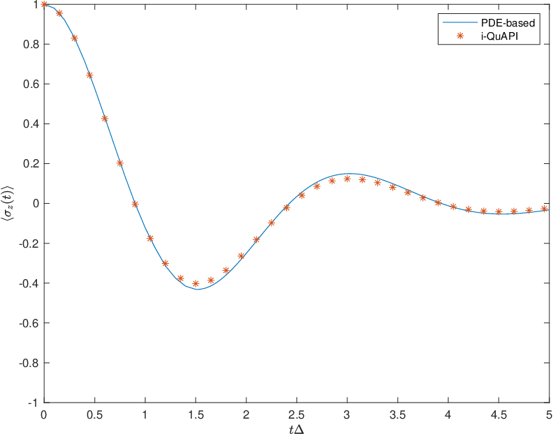
Refer to caption
(a) ξ=0.2\xi=0.2
Refer to caption
(b) ξ=0.4\xi=0.4
Figure 6. Both methods use truncation time T=1.5T=1.5. For i-QuAPI method, Δ​k\Delta k is chosen to be 10. For c-QuAPI, Dmax=8D_{\max}=8 and N=8N=8.

According to (40), it can be calculated that the DEBPI method needs to store Ndof=17444860N_{\mathrm{dof}}=17444860 different values of A⁡(t,h)A(t,h) for each time step. In comparison, the i-QuAPI method, which has a smaller grid size, only requires to store 22×10=10485762^{2\times 10}=1048576 different values. To understand such a difference, we note that each discrete path segment in the i-QuAPI method can also be represented using the initial state (r+,r−)(r^{+},r^{-}), the number of spin flips DD, the branches of the spin flips sgn\mathrm{sgn}, and the time difference between each pair of spin flips (τ1,⋯,τD)(\tau_{1},\cdots,\tau_{D}). However, for the i-QuAPI method, there are never more than one spin flip occurring at the same time on the same branch. In other words, if sgnk=sgnk+1\mathrm{sgn}_{k}=\mathrm{sgn}_{k+1}, then τk+1\tau_{k+1} must be nonzero. For example, when D=2D=2 and sgn1=sgn2\mathrm{sgn}_{1}=\mathrm{sgn}_{2}, the five points located on the vertical axis of Figure 5a are not considered in the i-QuAPI method, leading to a lower memory cost than that in our discretization. For larger DD, this will cause more significant difference in the memory usage even if the grid sizes for both methods are the same. This difference can be eliminated by using a smarter PDE solver, which will be studied to our future work.

Based on our current approach, the memory cost grows exponentially with DmaxD_{\max}. Therefore, if the problem setting allows a lower value of DmaxD_{\max}, the DEBPI method will show its advantage. Moreover, if DmaxD_{\max} can be chosen small, we can use a small grid size in the discretization of △T(D)\triangle_{T}^{(D)} to achieve better accuracy, while for the i-QuAPI method, the memory cost grows exponentially with Δ​k\Delta k, so that it is prohibitive to choose small grid sizes. In the following two subsections, we will show several cases with small spin-flipping frequency such that our method can achieve a lower memory cost.

5.2.2. Experiments with different biases

We now consider the following set of parameters:

ξ=0.2,Δ=0.2,ωc=5​Δ,β=5/Δ,\xi=0.2,\quad\Delta=0.2,\quad\omega_{c}=5\Delta,\quad\beta=5/\Delta,

where the spin flipping frequency Δ\Delta is smaller so we expect that a smaller DmaxD_{\max} can be adopted for our DEBPI approach. Three different biases ϵ\epsilon are chosen, and the results are given in Figure 7. For Dmax=5D_{\max}=5, the curves for the DEPBI method almost coincide with the i-QuAPI results. Since the parameter ϵ\epsilon denotes the difference between the energies of the two states, the three figures correctly show that when ϵ\epsilon is larger, the state of spin is more likely to be found as |−1⟩\ket{-1}, leading to the downshift of the curve in the second and third subplots in Figure 7.

Refer to caption
(a) ϵ=0\epsilon=0
Refer to caption
(b) ϵ=0.5​Δ\epsilon=0.5\Delta
Refer to caption
(c) ϵ=Δ\epsilon=\Delta
Figure 7. Both methods use truncation time T=4T=4. For i-QuAPI method, Δ​k\Delta k is chosen to be 10 and for c-QuAPI, Dmax=5D_{\max}=5 and N=10N=10.

In these tests, DEBPI needs ∑D=054×2D​(D+10D)=458748\displaystyle\sum_{D=0}^{5}4\times 2^{D}\begin{pmatrix}D+10\\ D\end{pmatrix}=458748 numbers to store the numerical solution, while the i-QuAPI scheme needs 22×10=10485762^{2\times 10}=1048576. Thus the memory cost of our method is about a half of the cost of i-QuAPI. Note that further reducing DmaxD_{\max} may cause significant error in the numerical solution. Figure 8 shows the numerical results for Dmax=3,4,5D_{\max}=3,4,5 when ϵ=0\epsilon=0, indicating that Dmax=5D_{\max}=5 is a proper choice to guarantee the quality of the solution.

Refer to caption
Figure 8. ϵ=0\epsilon=0 and Dmax=3,4,5D_{\max}=3,4,5.

In general, the parameter DmaxD_{\max} can be considered as a factor controlling the trade-off between the memory cost and the numerical accuracy. In order that DmaxD_{\max} can be chosen small, we need both the memory time and the spin flipping frequency to be relatively small, meaning that within the path segment TT, the spin is unlikely to flip many times. Under such circumstances, our method is more likely to outperform the method of i-QuAPI in terms of the memory cost.

5.2.3. Experiments with different temperatures

For the last set of tests, we choose the parameters

ξ=0.2,Δ=0.1,ωc=2.5​Δ,ϵ=0,\xi=0.2,\quad\Delta=0.1,\quad\omega_{c}=2.5\Delta,\quad\epsilon=0,

and we let the inverse temperature of the bath β\beta vary from 0.2/Δ0.2/\Delta to 5/Δ5/\Delta. The results and the numerical parameters are given in Figure 9. As reflected in the numerical results, in the case of higher temperature, stronger quantum dissipation leads to faster reduction to the state with equal probabilities on both spin states.

Refer to caption
(a) β=0.2/Δ\beta=0.2/\Delta
Refer to caption
(b) β=1/Δ\beta=1/\Delta
Refer to caption
(c) β=5/Δ\beta=5/\Delta
Figure 9. Both methods use truncation time T=4T=4. For i-QuAPI method, Δ​k\Delta k is chosen to be 10 and for c-QuAPI, Dmax=3D_{\max}=3 and N=15N=15.

Compared with the examples in Section 5.2.2, we use the same memory length T=4T=4, while the spin flipping frequency Δ\Delta is reduced by a half. Thus it can be expected that the value of DmaxD_{\max} can also be reduced by a half. Therefore, choosing Dmax=3D_{\max}=3 is sufficient to capture the behavior of evolution processes here. In these examples, due to the small value of DmaxD_{\max}, the memory cost of the DEBPI approach is much lower even if NN is chosen to be greater than Δ​k\Delta k. In detail, the DEBPI approach only requires to store ∑D=034×2D​(D+15D)=28420\displaystyle\sum_{D=0}^{3}4\times 2^{D}\begin{pmatrix}D+15\\ D\end{pmatrix}=28420 values, while the i-QuAPI scheme requires 22×10=10485762^{2\times 10}=1048576.

6. Conclusion and discussion

We have formulated a PDE system for open quantum systems with truncated memory length in the bath-influence functional. The PDE system is supplemented with proper initial and boundary conditions, and truncated with a reasonable closure. Such a formulation allows us to solve the density matrix using classical PDE-solvers for hyperbolic systems. By this approach, the memory cost can be saved in two possible ways. First, higher-order schemes can be applied to reduce the number of grid points. Second, in some situations, we can choose DmaxD_{\max} to be smaller than NN to avoid discretization of high-dimensional simplicies. In our numerical tests, we considered the second-order numerical schemes (the same as i-QuAPI), and illustrated several cases where DmaxD_{\max} can be chosen small. The higher-order schemes are being studied in our ongoing work.

While this paper focuses mainly on the spin-boson model, the idea of deriving the governing differential equations can be generalized to any quantum system with finite states without much difficulty. When 𝒮\mathcal{S} contains more elements, the representation of the path segments will be slightly more complicated. In detail, the path segment hh cannot be fully determined by the initial state and the locations of state hops. Instead, it is necessary to specify which state the system hops to at each τk\tau_{k}. Nevertheless, the idea to derive the PDE system and the expression of density matrix stays the same. Roughly speaking, the equation of A⁡(t,h)A(t,h) holds the form

(41) ∂∂t​A​(t,h)=−W⁡(h)​A​(t,h)+∑h^A⁡(t,h^)+∂∂τ1​A​(t,h),\frac{\partial}{\partial t}A(t,h)=-W(h)A(t,h)+\sum_{\hat{h}}A(t,\hat{h})+\frac{\partial}{\partial\tau_{1}}A(t,h),

where τ1\tau_{1} is the location of the first state hop in hh, and the path segment h^\hat{h} takes all possible paths satisfying h^​(τ)=h​(τ)\hat{h}(\tau)=h(\tau) for all τ∈(0,T)\tau\in(0,T) and

h^+​(0)=h^+​(0)​ and ​h^−​(0)≠h^−​(0)orh^+​(0)≠h^+​(0)​ and ​h^−​(0)=h^−​(0).\hat{h}^{+}(0)=\hat{h}^{+}(0)\text{ and }\hat{h}^{-}(0)\neq\hat{h}^{-}(0)\qquad\text{or}\qquad\hat{h}^{+}(0)\neq\hat{h}^{+}(0)\text{ and }\hat{h}^{-}(0)=\hat{h}^{-}(0).

The equation (41) is essentially the same as (29) in the spin-boson case. However, when the cardinality of 𝒮\mathcal{S} is larger, the memory cost also grows faster with DmaxD_{\max} and NN, requiring more efficient numerical methods for the simulation. This will be considered in our future works.

Appendix. Derivation of i-QuAPI Method

A component of the reduced density matrix ρs\rho_{s} at time t=N​Δ​tt=N\Delta t, denoted by ⟨s′′|ρs​(N​Δ​t)|s′⟩\matrixelement{s''}{\rho_s(N\dt)}{s'}, can be represented by

⟨s′′|ρs​(N​Δ​t)|s′⟩=trb​⟨s′′|e−i​H​N​Δ​t​ρ​(0)​ei​H​N​Δ​t|s′⟩.\matrixelement{s''}{\rho_s(N\dt)}{s'}=\tr_{b}\matrixelement{s''}{\e^{-\ii H N\dt} \rho(0) \e^{\ii H N \dt}}{s'}.

With the completeness relation in a quantum system

∫𝒮|s⟩⟨s|​𝑑s=ids,\int_{\mathcal{S}}\outerproduct{s}{s}\mathrm{d}s=\mathrm{id}_{s},

with 𝒮\mathcal{S} being the set of an orthonormal basis, the reduced density matrix can be written as a path integral form

⟨s′′|ρs​(N​Δ​t)|s′⟩=trb∫𝒮ds0+⋯∫𝒮dsN−1+∫𝒮ds0−⋯∫𝒮dsN−1+⟨s′′|e−i​H​Δ​t|sN−1+⟩⟨sN−1+|e−i​H​Δ​t|sN−2+⟩⋯⟨s1+|e−i​H​Δ​t|s0+⟩⟨s0+|ρ⁡(0)|s0−⟩⟨s0−|ei​H​Δ​t|s1−⟩⋯⟨sN−2+|ei​H​Δ​t|sN−1−⟩⟨sN−1−|ei​H​Δ​t|s′⟩.\begin{split}\matrixelement{s''}{\rho_s(N\dt)}{s'}=&\tr_{b}\int_{\mathcal{S}}\mathrm{d}s_{0}^{+}\cdots\int_{\mathcal{S}}\mathrm{d}s_{N-1}^{+}\int_{\mathcal{S}}\mathrm{d}s_{0}^{-}\cdots\int_{\mathcal{S}}\mathrm{d}s_{N-1}^{+}\matrixelement{s''}{\e^{-\ii H \dt}}{s_{N-1}^+}\\ &\matrixelement{s_{N-1}^+}{\e^{-\ii H \dt}}{s_{N-2}^+}\cdots\matrixelement{s_1^+}{\e^{-\ii H \dt}}{s_0^+}\matrixelement{s_0^+}{\rho(0)}{s_0^-}\\ &\matrixelement{s_0^-}{\e^{\ii H \dt}}{s_1^-}\cdots\matrixelement{s_{N-2}^+}{\e^{\ii H \dt}}{s_{N-1}^-}\matrixelement{s_{N-1}^-}{\e^{\ii H \dt}}{s'}.\end{split}

(Appendix. Derivation of i-QuAPI Method) is called path integral as the states s0+,⋯,sN+s_{0}^{+},\cdots,s_{N}^{+} and s0−,⋯,sN−s_{0}^{-},\cdots,s_{N}^{-} can be regarded as a path, an integral over all possible paths are taken here. It is clear that the path has two branches (positive branch and negative branch).

For the spin-boson model, 𝒮={−1,+1}\mathcal{S}=\{-1,+1\}, therefore, Appendix. Derivation of i-QuAPI Method becomes

⟨s′′|ρs​(N​Δ​t)|s′⟩=\displaystyle\matrixelement{s''}{\rho_s(N\dt)}{s'}= trb∑s0+=±1⋯∑sN−1+=±1∑s0−=±1⋯∑sN−1−=±1⟨s′′|e−i​H​Δ​t|sN−1+⟩\displaystyle\tr_{b}\sum_{s_{0}^{+}=\pm 1}\cdots\sum_{s_{N-1}^{+}=\pm 1}\sum_{s_{0}^{-}=\pm 1}\cdots\sum_{s_{N-1}^{-}=\pm 1}\matrixelement{s''}{\e^{-\ii H \dt}}{s_{N-1}^+}
⟨sN−1+|e−i​H​Δ​t|sN−2+⟩⋯⟨s1+|e−i​H​Δ​t|s0+⟩⟨s0+|ρ⁡(0)|s0−⟩\displaystyle\matrixelement{s_{N-1}^+}{\e^{-\ii H \dt}}{s_{N-2}^+}\cdots\matrixelement{s_1^+}{\e^{-\ii H \dt}}{s_0^+}\matrixelement{s_0^+}{\rho(0)}{s_0^-}
⟨s0−|ei​H​Δ​t|s1−⟩⋯⟨sN−2+|ei​H​Δ​t|sN−1−⟩⟨sN−1−|ei​H​Δ​t|s′⟩.\displaystyle\matrixelement{s_0^-}{\e^{\ii H \dt}}{s_1^-}\cdots\matrixelement{s_{N-2}^+}{\e^{\ii H \dt}}{s_{N-1}^-}\matrixelement{s_{N-1}^-}{\e^{\ii H \dt}}{s'}.

As for the special Hamiltonian given by (2), Trotter splitting can be used by introducing the following reference Hamiltonian

(42) H0=(ϵ​σ^z+Δ​σ^x−∑j(cj​σ^z)22​ωj2)⊗idb.H_{0}=\left(\epsilon\hat{\sigma}_{z}+\Delta\hat{\sigma}_{x}-\sum_{j}\frac{(c_{j}\hat{\sigma}_{z})^{2}}{2\omega_{j}^{2}}\right)\otimes\mathrm{id}_{b}.

Therefore, the remaining part is

H−H0=∑j(ids⊗p^j22+12​ωj2​(ids⊗q^j−cjωj2​σ^z⊗idb)2).H-H_{0}=\sum_{j}\left(\mathrm{id}_{s}\otimes\frac{\hat{p}_{j}^{2}}{2}+\frac{1}{2}\omega_{j}^{2}\left(\mathrm{id}_{s}\otimes\hat{q}_{j}-\frac{c_{j}}{\omega_{j}^{2}}\hat{\sigma}_{z}\otimes\mathrm{id}_{b}\right)^{2}\right).

When the splitting is applied, the reduced density matrix can be written as

⟨s′′|ρs​(N​Δ​t)|s′⟩=\displaystyle\matrixelement{s''}{\rho_s(N\dt)}{s'}= ∑s0+=±1⋯∑sN−1+=±1∑s0−=±1⋯∑sN−1−=±1⟨s′′|e−i​H​Δ​t|sN−1+⟩\displaystyle\sum_{s_{0}^{+}=\pm 1}\cdots\sum_{s_{N-1}^{+}=\pm 1}\sum_{s_{0}^{-}=\pm 1}\cdots\sum_{s_{N-1}^{-}=\pm 1}\matrixelement{s''}{\e^{-\ii H \dt}}{s_{N-1}^+}
⟨sN−1+|e−i​H​Δ​t|sN−2+⟩⋯⟨s1+|e−i​H​Δ​t|s0+⟩⟨s0+|ρs​(0)|s0−⟩\displaystyle\matrixelement{s_{N-1}^+}{\e^{-\ii H \dt}}{s_{N-2}^+}\cdots\matrixelement{s_1^+}{\e^{-\ii H \dt}}{s_0^+}\matrixelement{s_0^+}{\rho_s(0)}{s_0^-}
⟨s0−|ei​H​Δ​t|s1−⟩⋯⟨sN−2+|ei​H​Δ​t|sN−1−⟩⟨sN−1−|ei​H​Δ​t|s′⟩\displaystyle\matrixelement{s_0^-}{\e^{\ii H \dt}}{s_1^-}\cdots\matrixelement{s_{N-2}^+}{\e^{\ii H \dt}}{s_{N-1}^-}\matrixelement{s_{N-1}^-}{\e^{\ii H \dt}}{s'}
F⁡(s0+,s1+,⋯,sN+,s0−,s1−,⋯,sN−)\displaystyle F(s_{0}^{+},s_{1}^{+},\cdots,s_{N}^{+},s_{0}^{-},s_{1}^{-},\cdots,s_{N}^{-})

with sN+=s′′,sN−=s′s_{N}^{+}=s^{\prime\prime},s_{N}^{-}=s^{\prime} and

F⁡(s0+,s1+,⋯,sN+,s0−,s1−,⋯,sN−)=trb[e−i​Δ​t2​(H−H0​(s′′))e−i​Δ​t​(H−H0​(sN−1+))⋯e−i​Δ​t​(H−H0​(s1+))e−i​Δ​t2​(H−H0​(s0+))ρb(0)ei​Δ​t2​(H−H0​(s0−))ei​Δ​t​(H−H0​(s1−))⋯ei​Δ​t​(H−H0​(sN−1−))ei​Δ​t2​(H−H0​(s′))].\begin{split}&F(s_{0}^{+},s_{1}^{+},\cdots,s_{N}^{+},s_{0}^{-},s_{1}^{-},\cdots,s_{N}^{-})\\ =&\tr_{b}\left[\mathrm{e}^{-\mathrm{i}\frac{\Delta t}{2}(H-H_{0}(s^{\prime\prime}))}\mathrm{e}^{-\mathrm{i}\Delta t(H-H_{0}(s_{N-1}^{+}))}\cdots\mathrm{e}^{-\mathrm{i}\Delta t(H-H_{0}(s_{1}^{+}))}\right.\\ &\mathrm{e}^{-\mathrm{i}\frac{\Delta t}{2}(H-H_{0}(s_{0}^{+}))}\rho_{b}(0)\mathrm{e}^{\mathrm{i}\frac{\Delta t}{2}(H-H_{0}(s_{0}^{-}))}\mathrm{e}^{\mathrm{i}\Delta t(H-H_{0}(s_{1}^{-}))}\cdots\\ &\left.\mathrm{e}^{\mathrm{i}\Delta t(H-H_{0}(s_{N-1}^{-}))}\mathrm{e}^{\mathrm{i}\frac{\Delta t}{2}(H-H_{0}(s^{\prime}))}\right].\end{split}

The function FF is called influence functional, calculating the influence of the environment on the system of interest. With (42) as reference Hamiltonian, the influence functional can be computed analytically [5][14] by

(43) F(s0+,⋯,sN+,s0−,⋯,sN−)=exp(−∑j1=0N∑j2=0j1(sj1+−sj1−)(ηj1,j2sj2+−ηj1,j2∗sj2−)).F(s_{0}^{+},\cdots,s_{N}^{+},s_{0}^{-},\cdots,s_{N}^{-})=\exp\left(-\sum_{j_{1}=0}^{N}\sum_{j_{2}=0}^{j_{1}}(s_{j_{1}}^{+}-s_{j_{1}}^{-})(\eta_{j_{1},j_{2}}s_{j_{2}}^{+}-\eta_{j_{1},j_{2}}^{*}s_{j_{2}}^{-})\right).

In the influence functional (43), η\eta is a complex function and η∗\eta^{*} is its complex conjugate. For different j1,j2j_{1},j_{2}, η\eta has different forms [19]. For example, when 0<j2<j1<N0<j_{2}<j_{1}<N, we have

ηj1,j2=2π​∫−∞∞d​ω​J⁡(ω)ω2​exp⁡(ω​β/2)sinh⁡(ω​β/2)​sin2⁡(ω​Δ​t/2)​exp⁡(−i⁡(j1−j2)​ω​Δ​t)\eta_{j_{1},j_{2}}=\frac{2}{\pi}\int_{-\infty}^{\infty}\mathrm{d}\omega\frac{J(\omega)}{\omega^{2}}\frac{\exp(\omega\beta/2)}{\sinh(\omega\beta/2)}\sin^{2}(\omega\Delta t/2)\exp\left(-\mathrm{i}(j_{1}-j_{2})\omega\Delta t\right)

where

J⁡(ω)=π2​∑jcj2mj​ωj​δ​(ω−ωj)J(\omega)=\frac{\pi}{2}\sum_{j}\frac{c_{j}^{2}}{m_{j}\omega_{j}}\delta(\omega-\omega_{j})

and δ\delta is the Dirac delta function.

The absolute value of η\eta decreases to zero as j1−j2j_{1}-j_{2} increases. Thus, when the difference of j1j_{1} and j2j_{2} is large, the contribution of ηj1,j2\eta_{j_{1},j_{2}} is small. From this point of view, the influence functional can be approximated by

F(s0+,⋯,sN+,s0−,⋯,sN−)≈exp(−∑j1=0N∑j2=max⁡{0,k−Δ​k}j1(sj1+−sj1−)(ηj1−j2sj2+−ηj1−j2∗sj2−)).F(s_{0}^{+},\cdots,s_{N}^{+},s_{0}^{-},\cdots,s_{N}^{-})\approx\exp\left(-\sum_{j_{1}=0}^{N}\sum_{j_{2}=\max\{0,k-\Delta k\}}^{j_{1}}(s_{j_{1}}^{+}-s_{j_{1}}^{-})(\eta_{j_{1}-j_{2}}s_{j_{2}}^{+}-\eta_{j_{1}-j_{2}}^{*}s_{j_{2}}^{-})\right).

For simplicity, the notation Sj=(sj+,sj−)S_{j}=(s_{j}^{+},s_{j}^{-}) is introduced and the notation I(Sj,Sj′)I_{(S_{j},S_{j^{\prime}})} is defined by

I⁡(Sj,Sj′)={e−(sj+−sj−)​(ηj,j′​sj′+−ηj,j′∗​sj′−),j−j′≠1⟨sj+|e−i​H0​Δ​t|sj−1+⟩​⟨sj−1−|ei​H0​Δ​t|sj−⟩​e−(sj+−sj−)​(ηj,j′​sj′+−ηj,j′∗​sj′−),j−j′=1.I(S_{j},S_{j^{\prime}})=\begin{cases}\mathrm{e}^{-(s_{j}^{+}-s_{j}^{-})(\eta_{j,j^{\prime}}s_{j^{\prime}}^{+}-\eta_{j,j^{\prime}}^{*}s_{j^{\prime}}^{-})},\quad j-j^{\prime}\not=1\\ \matrixelement{s_j^+}{\e^{-\ii H_0 \dt}}{s_{j-1}^+}\matrixelement{s_{j-1}^-}{\e^{\ii H_0\dt}}{s_j^-}\mathrm{e}^{-(s_{j}^{+}-s_{j}^{-})(\eta_{j,j^{\prime}}s_{j^{\prime}}^{+}-\eta_{j,j^{\prime}}^{*}s_{j^{\prime}}^{-})},\quad j-j^{\prime}=1\end{cases}.

With these notations,

(44) ρ~​(SN,N​Δ​t)=∑SN−1⋯∑S0∏j1=0N∏j2=0j1I(Sj1,Sj2)⟨s0+|ρs​(0)|s0−⟩=∑SN−1⋯∑S0(∏j=Δ​kN∏m=0Δ​kI(Sj,Sj−m))(∏k1=0Δ​k−1∏k2=0k1I⁡(Sj1,Sj2)​⟨s0+|ρs​(0)|s0−⟩)⏟:=A0​(SΔ​k−1,⋯,S0)=∑SN−1⋯∑S1(∑j=Δ​k+1N∑m=0kI(Sj,Sj−m))∑S0(∏m=0Δ​kI⁡(SΔ​k,SΔ​k−m))⏟:=Λ⁡(SΔ​k,⋯,S0)A0(SΔ​k−1,⋯,S0)⏟:=A1​(SΔ​k,⋯,S1)=∑SN−1⋯∑S2(∑j=Δ​k+2N∑m=0kI(Sj,Sj−m))∑S1∏m=0Δ​kI⁡(SΔ​k+1,SΔ​k+1−m)⏟:=Λ⁡(SΔ​k+1,⋯,S1)A1(SΔ​k,⋯,S1)⏟:=A2​(SΔ​k+1,⋯,S2)=⋯\begin{split}&\tilde{\rho}(S_{N};N\Delta t)\\ =&\sum_{S_{N-1}}\cdots\sum_{S_{0}}\prod_{j_{1}=0}^{N}\prod_{j_{2}=0}^{j_{1}}I(S_{j_{1}},S_{j_{2}})\matrixelement{s_0^+}{\rho_s(0)}{s_0^-}\\ =&\sum_{S_{N-1}}\cdots\sum_{S_{0}}\left(\prod_{j=\Delta k}^{N}\prod_{m=0}^{\Delta k}I(S_{j},S_{j-m})\right)\underbrace{\left(\prod_{k_{1}=0}^{\Delta k-1}\prod_{k_{2}=0}^{k_{1}}I(S_{j_{1}},S_{j_{2}})\matrixelement{s_0^+}{\rho_s(0)}{s_0^-}\right)}_{:=A_{0}(S_{\Delta k-1},\cdots,S_{0})}\\ =&\sum_{S_{N-1}}\cdots\sum_{S_{1}}\left(\sum_{j=\Delta k+1}^{N}\sum_{m=0}^{k}I(S_{j},S_{j-m})\right)\underbrace{\sum_{S_{0}}\underbrace{\left(\prod_{m=0}^{\Delta k}I(S_{\Delta k},S_{\Delta k-m})\right)}_{:=\Lambda(S_{\Delta k},\cdots,S_{0})}A_{0}(S_{\Delta k-1},\cdots,S_{0})}_{:=A_{1}(S_{\Delta k},\cdots,S_{1})}\\ =&\sum_{S_{N-1}}\cdots\sum_{S_{2}}\left(\sum_{j=\Delta k+2}^{N}\sum_{m=0}^{k}I(S_{j},S_{j-m})\right)\underbrace{\sum_{S_{1}}\underbrace{\prod_{m=0}^{\Delta k}I(S_{\Delta k+1},S_{\Delta k+1-m})}_{:=\Lambda(S_{\Delta k+1},\cdots,S_{1})}A_{1}(S_{\Delta k},\cdots,S_{1})}_{:=A_{2}(S_{\Delta k+1},\cdots,S_{2})}\\ =&\cdots\end{split}

An iterative method (i-QuAPI) is designed [13][14] according to (44) as follows.

A0​(SΔ​k−1,⋯,S0):=∏k1=0Δ​k−1∏k2=0kI⁡(Sk1,Sk2)​⟨s0+|ρs​(0)|s0−⟩;\displaystyle A_{0}(S_{\Delta k-1},\cdots,S_{0}):=\prod_{k_{1}=0}^{\Delta k-1}\prod_{k_{2}=0}^{k}I(S_{k_{1}},S_{k_{2}})\matrixelement{s_0^+}{\rho_s(0)}{s_0^-};
Λ⁡(Sk,⋯,Sk−Δ​k):=∏m=0Δ​kI⁡(Sk,Sk−m);\displaystyle\Lambda(S_{k},\cdots,S_{k-\Delta k}):=\prod_{m=0}^{\Delta k}I(S_{k},S_{k-m});
Ak+Δ​k+1​(Sk,⋯,Sk−Δ​k+1):=∑Sk−Δ​kΛ⁡(Sk,⋯,Sk−Δ​k)​Ak−Δ​k​(Sk−1,⋯,Sk−Δ​k).\displaystyle A_{k+\Delta k+1}(S_{k},\cdots,S_{k-\Delta k+1}):=\sum_{S_{k-\Delta k}}\Lambda(S_{k},\cdots,S_{k-\Delta k})A_{k-\Delta k}(S_{k-1},\cdots,S_{k-\Delta k}).

The density matrix then can be obtained component-wise by

⟨sN+|ρs​(N​Δ​t)|sN−⟩=∑SN−Δ​k+1,⋯,SN−1AN−Δ​k​(SN,⋯,SN−Δ​k+1).\matrixelement{s_N^+}{{\rho}_s(N\dt)}{s_N^-}=\sum_{S_{N-\Delta k+1},\cdots,S_{N-1}}A_{N-\Delta k}(S_{N},\cdots,S_{N-\Delta k+1}).

With a density matrix of the system, the expected value of any observable OO of the system can be computed by

⟨O⁡(t)⟩=tr⁡(ρs​(t)​O).\expectationvalue{O(t)}=\tr(\rho_s(t)O).

In spin-boson model, the density matrix ρs​(t)\rho_{s}(t) is a two-by-two matrix and the observable OO is also a two-by-two matrix.

References

  • [1] Z. Cai, J. Lu, and S. Yang. Inchworm Monte Carlo method for open quantum systems. Communications on Pure and Applied Mathematics, 73(11):2430–2472, 2020.
  • [2] Z. Cai, J. Lu, and S. Yang. Numerical analysis for inchworm Monte Carlo method: sign problem and error growth. arXiv preprint arXiv:2006.07654, 2020.
  • [3] H. Carmichael. An open systems approach to quantum optics: lectures presented at the Université Libre de Bruxelles, October 28 to November 4, 1991, volume 18. Springer Science & Business Media, 2009.
  • [4] H.-T. Chen, G. Cohen, and D. R. Reichman. Inchworm Monte Carlo for exact non-adiabatic dynamics. i. theory and algorithms. The Journal of chemical physics, 146(5):054105, 2017.
  • [5] R. Feynman and F. Vernon. The theory of a general quantum system interacting with a linear dissipative system. Annals of Physics, 24:118–173, 1963.
  • [6] V. Gorini, A. Kossakowski, and E. C. G. Sudarshan. Completely positive dynamical semigroups of n-level systems. Journal of Mathematical Physics, 17(5):821–825, 1976.
  • [7] A. Kelly and T. E. Markland. Efficient and accurate surface hopping for long time nonadiabatic quantum dynamics. The Journal of Chemical Physics, 139(1):014104, 2013.
  • [8] P. Khrennikova, E. Haven, and A. Khrennikov. An application of the theory of open quantum systems to model the dynamics of party governance in the US political system. International journal of theoretical physics, 53(4):1346–1360, 2014.
  • [9] A. J. Leggett, S. Chakravarty, A. T. Dorsey, M. P. Fisher, A. Garg, and W. Zwerger. Dynamics of the dissipative two-state system. Reviews of Modern Physics, 59(1):1, 1987.
  • [10] G. Lindblad. On the generators of quantum dynamical semigroups. Communications in Mathematical Physics, 48(2):119–130, 1976.
  • [11] E. Loh Jr, J. Gubernatis, R. Scalettar, S. White, D. Scalapino, and R. Sugar. Sign problem in the numerical simulation of many-electron systems. Physical Review B, 41(13):9301, 1990.
  • [12] N. Makri. Improved Feynman propagators on a grid and non-adiabatic corrections within the path integral framework. Chemical physics letters, 193(5):435–445, 1992.
  • [13] N. Makri. Numerical path integral techniques for long time dynamics of quantum dissipative systems. Journal of Mathematical Physics, 36(5):2430–2457, 1995.
  • [14] N. Makri. Quantum dissipative dynamics: A numerically exact methodology. The Journal of Physical Chemistry A, 102(24):4414–4427, 1998.
  • [15] N. Makri. The linear response approximation and its lowest order corrections: An influence functional approach. The Journal of Physical Chemistry B, 103(15):2823–2829, 1999.
  • [16] N. Makri. Blip decomposition of the path integral: Exponential acceleration of real-time calculations on quantum dissipative systems. The Journal of chemical physics, 141(13):134117, 2014.
  • [17] N. Makri. Blip-summed quantum–classical path integral with cumulative quantum memory. Faraday discussions, 195:81–92, 2017.
  • [18] N. Makri. Small matrix path integral for system-bath dynamics. Journal of Chemical Theory and Computation, 16(7):4038–4049, 2020.
  • [19] N. Makri and D. E. Makarov. Tensor propagator for iterative quantum time evolution of reduced density matrices. i. theory. The Journal of chemical physics, 102(11):4600–4610, 1995.
  • [20] S. Nakajima. On quantum theory of transport phenomena: Steady diffusion. Progress of Theoretical Physics, 20(6):948–959, 1958.
  • [21] M. A. Nielsen and I. Chuang. Quantum computation and quantum information, 2002.
  • [22] A. Shabani and D. A. Lidar. Completely positive post-markovian master equation via a measurement approach. Physical Review A, 71(2):020101, 2005.
  • [23] E. Sim and N. Makri. Tensor propagator with weight-selected paths for quantum dissipative dynamics with long-memory kernels. Chemical physics letters, 249(3-4):224–230, 1996.
  • [24] J. Strümpfer and K. Schulten. Open quantum dynamics calculations with the hierarchy equations of motion on parallel computers. Journal of chemical theory and computation, 8(8):2808–2816, 2012.
  • [25] Y. Tanimura and R. Kubo. Two-time correlation functions of a system coupled to a heat bath with a Gaussian-Markoffian interaction. Journal of the Physical Society of Japan, 58(4):1199–1206, 1989.
  • [26] B. Vacchini and H.-P. Breuer. Exact master equations for the non-markovian decay of a qubit. Physical Review A, 81(4):042103, 2010.
  • [27] U. Weiss. Quantum dissipative systems, volume 13. World scientific, 2012.
  • [28] P. Werner, T. Oka, and A. J. Millis. Diagrammatic Monte Carlo simulation of nonequilibrium systems. Physical Review B, 79(3):035320, 2009.
  • [29] S. Yang, Z. Cai, and J. Lu. Inclusion–exclusion principle for open quantum systems with bosonic bath. New Journal of Physics, 23(6):063049, 2021.
  • [30] R. Zwanzig. Ensemble method in the theory of irreversibility. The Journal of Chemical Physics, 33(5):1338–1341, 1960.