Multiple Query Optimization using a Hybrid Approach of Classical and Quantum Computing
Abstract
Quantum computing promises to solve difficult optimization problems in chemistry, physics and mathematics more efficiently than classical computers, but requires fault-tolerant quantum computers with millions of qubits. To overcome errors introduced by today’s quantum computers, hybrid algorithms combining classical and quantum computers are used.
In this paper we tackle the multiple query optimization problem (MQO) which is an important NP-hard problem in the area of data-intensive problems. We propose a novel hybrid classical-quantum algorithm to solve the MQO on a gate-based quantum computer. We perform a detailed experimental evaluation of our algorithm and compare its performance against a competing approach that employs a quantum annealer – another type of quantum computer. Our experimental results demonstrate that our algorithm currently can only handle small problem sizes due to the limited number of qubits available on a gate-based quantum computer compared to a quantum computer based on quantum annealing. However, our algorithm shows a qubit efficiency of close to 99% which is almost a factor of 2 higher compared to the state of the art implementation. Finally, we analyze how our algorithm scales with larger problem sizes and conclude that our approach shows promising results for near-term quantum computers.
1 Introduction
In database research, various optimization problems have been formulated since the seventies [35, 22, 37], with the query optimization problem being a typical NP-hard representative. These problems, although extensively examined, become even more difficult as data processing becomes more complex [40]. Recent approaches to the query optimization problem have also become increasingly sophisticated, now employing deep learning methods [22, 28]. Simultaneously, progress in the construction of quantum computers has sparked new interest in applied quantum computing [6, 12, 4, 32], whereas previously, the quantum computing community was mainly concerned with more theoretical studies due to the lack of practical quantum devices [30]. It is hoped that quantum computers can one day solve complex problems more efficiently than classical computers [30].
Although quantum computers were first envisioned to simulate quantum systems [15], the first two famous use cases were outside of physics. Namely, search in an unstructured list [19] and factoring large integers [38].
More recently, quantum computers are considered for mathematical optimization [12], or simulation of molecules for chemistry [32]. Current quantum computers are still in their infancy and are restricted by the capacity and fault-tolerance [30, 4, 43], making them more interesting for quantum research than for real-world application. This motivated the creation of hybrid classical-quantum algorithms like the Quantum Approximate Optimization Algorithm (QAOA) [12] that employ a quantum device to explore high-dimensional search space and classical routines to optimize the search procedure. By only relaying parts of the computation to the quantum computers, these hybrid classical-quantum-algorithms are more resistant to error [12], making them more suitable to near-term devices.
The Multiple Query Optimization problem (MQO) is a generalization of the query optimization problem [37]. MQO is known to be an NP-hard problem [36]. It has been approached by classical methods such as the shortest-path algorithms [37], genetic algorithms [5] and others. Recently, a quantum approach was suggested for the MQO by Trummer and Koch [40], utilizing a D-Wave quantum annealer [10], a particular type of quantum computer designed to run special optimization problems [40]. Our work builds on Trummer and Koch’s approach, but utilizes a gate-based quantum computer, a more general type of quantum computer. Gate-based quantum computers can, in principle, run every quantum algorithm [2, 24], while quantum annealers are restricted to specific problems [40]. This advantage comes with the cost that gate-based quantum computers currently feature significantly fewer qubits and are more error-prone than quantum annealers.
1.1 Multiple Query Optimization
Multiple query optimization (MQO) aims to minimize the total cost of executing a series of queries against a database by exploiting shared intermediate results [37].
Example 1
Consider a database with tables of different sizes. On these tables, queries can be formulated, such as . To produce this query, there may exist multiple plans that vary in the order of joins, order of selections and other aspects. For example, selections are usually done before joining tables to reduce the number of operations required for the join. Figure 1 shows two of those plans.
Our model considers a series of queries , where each query has a fixed number of plans, uniquely identified as . For every query, exactly one plan has to be selected. Each plan has associated a cost , which our model assumes as given.
Finally, we denote savings (e.g. from shared intermediate results) pairwise between plans and as . Savings can be subtracted from the total cost if both plans from the pair have been selected.
In the below example, the pairs of plans , have savings as they can use an intermediate result from sharing a common table . The goal is to find a selection of plans for all the queries, such that the overall cost is minimized.
| , , | , , | , , | |
|---|---|---|---|
The search space of this problem is significant as there are possibilities to choose from for every query, resulting in possibilities overall11 1 If no savings were given, the least-cost solution is trivially obtained by selecting the least-cost plan of every query.. Informally, we can formulate the following rules to constrain the search space:
-
Plans with lower cost are preferred.
-
Cost savings across any queries are taken into consideration.
-
Exactly one plan is selected per query.
Example 2
We consider two queries , produced by plans and and , produced by plans and . The cost for the plans are and . When plans and are both selected, they save costs of . To find the least-cost solution, we compute the cost of every admissible selection as displayed below. That is, we only list solutions that feature exactly one plan per query.
Obviously, selecting plans and is the least-cost solution.
| Cost | ||
|---|---|---|
| , | , | |
| , | , | |
| , | , | |
| , | , |
1.2 Contributions of the Paper
The MQO scales exponentially with the number of query plans it contains [40]. While classical computing typically approaches such problems by pruning the search space [40], quantum computers can explore the entire search space simultaneously [31, 30].
In Section 2 we revise the most important foundations of quantum computing that are important for solving optimization problems such as multiple-query optimization.
In Section 3 we first show a classical brute-force approach for the MQO that enumerates and then evaluates every solution. We then provide an intuition for the quantum query optimization by characterizing the optimal solution in a way that can later be used for a quantum circuit, which is the quantum-equivalent to classical machine language. Finally, we show a high-level overview of our algorithm.
In Section 4, we first provide the necessary conceptual groundwork for the Quantum Approximate Optimization Algorithm (QAOA), on which the algorithm is based on, and establish the relationship to quantum annealing. Next, we formulate the MQO mathematically, translate it into a quantum circuit while simultaneously introducing the classic part of our algorithm. We conclude that section with a more refined low-level algorithm and a discussion about how the algorithm is run.
Finally, in Section 5, we present experimental results of our algorithm. As the algorithm’s performance relies heavily on the classical optimization part, we utilize novel optimization strategies that we analyze. Furthermore, we compare our approach with the quantum annealing approach to the MQO and demonstrate that our approach shows more efficient usage of qubits which is an advantage for future, more powerful gate-based quantum computers. We complete our results with a complexity analysis of our approach.
In summary, our contributions are the following:
- 1.
We provide a novel hybrid classical-quantum algorithm to solve the multiple query optimization. The only previous quantum computing-based approach tackling the multiple query optimization used a quantum annealer architecture [40]. To the best of our knowledge, this is the first paper in the literature to address the multiple query optimization problem with a gate-based quantum computer.
- 2.
We conduct experiments with the algorithm with real quantum hardware and simulators, and analyze how the algorithm scales with the problem size.
- 3.
We compare our work with a competing quantum query optimization approach.
2 Quantum Computing Foundations
Quantum algorithms are known for speeding up certain computations, such as integer factorization [31]. In principle, these algorithms achieve the significant speedup by not having to examine every branch in the search space sequentially, as by a classical brute force approach22 2 The conception of a quantum computer evaluating the entire search space in parallel and selecting the best solution is an incorrect oversimplification [1].. Instead, a quantum computer holds a large number of branches during computation, which is possible due to the fact that a quantum register can be understood as a superposition of basis states.
Here, we must add a brief excursion. Certain types of quantum systems, e.g. electrons or polarized photons, are in quantum mechanics represented by a data structure that is equivalent to a normalized vector in a two-dimensional complex vector space (i.e. a two-dimensional complex Hilbert space, to be precise). Such vectors, denoted by a so called ket , are the superposition of two basis vectors and :
| (1) |
whereby and
| (2) |
The data structure is called a qubit. Without delving into mathematical and physical details: qubits can be combined and then form a so called quantum register. If one has coupled qubits, the resulting quantum register is again a normalized element of a complex Hilbert space, whereby this space has dimension . A basis state of this Hilbert space can be understood as a bit sequence with . The bit sequence of the basis state encodes a natural number , therefore the basis states are often just written as with . A quantum register is then a superposition of basis states:
| (3) |
with
| (4) |
One aspect of superposition is so called quantum parallelism: One can understand an operation on a quantum register as the simultaneous operation on many basis states. This interpretation is sensible, because quantum operations are (in a mathematical sense) linear operations in a vector space that is built up from basis states. Another aspect (not explicitly discussed in this paper but relevant for many theoretical features of quantum computing) is due to the fact that quantum registers represent entangled states. A quantum computation is ended by some sort of quantum measurement. In brief, a quantum algorithm manipulates quantum registers with the goal of amplifying the probability of measuring the basis state (bit strings) that represents the solution to the problem under investigation.
The time development of a quantum state is described by the Schrödinger equation:
| (5) |
Thereby, is an operator (here a -dimensional matrix). The matrix is called the Hamiltonian of the system and is related to the system’s energy. Mathematically, is a so - called Hermitian matrix, which means that its eigenvalues are all real numbers. These eigenvalues are the energies of the respective eigenstate: If is an eigenstate of and the eigenvalue of , then the system carries energy if it is in state . The state with the lowest energy (the smallest ) is called the ground state.
The time evolution described by Equation 5 is not the only process of relevance in quantum computing. There are also so called measurements. For our purposes, it is sufficient to define a measurement as a stochastic, non-linear operation that transforms a general quantum register into one, randomly chosen basis state. Formally, a measurement is defined by (we use the notation of Equation 3):
| (6) |
This means that a measurement destroys the information stored in a quantum register, at least to some extent. That is the reason, why many algorithms in quantum computing can be understood as amplification processes for the basis state that represents the solution one is looking for (or geometrically speaking, rotate a general state towards the solution state by reducing the angle between a general state and the solution).
Equation 5 describes the temporal development of the system under consideration. One can show that the fact that is Hermitian leads to time evolution that preserves the length of the vector describing the state of the system. An operation that preserves the length of a vector is simply a rotation (though in high-dimensional vector space). An operator that mediates such a rotation is called unitary. The time evolution of a quantum mechanical system is therefore a unitary process. Process steps in quantum computing consist of unitary operations; one physical challenge one faces is to implement the Hamiltonian that belongs to a desired unitary operation .
Note well that the unitary time evolution given by Equation 5 is reversible, whereas a measurement by Equation 6 is an irreversible process.
Finally, we point out that even if the Hilbert space that describes a quantum register may be of high dimension, it is still a finite dimensional space. That means that the mathematics one needs for quantum computing is (comparably) simple; linear algebra is sufficient. The subtleties of linear functional analysis (colloquially linear algebra in infinite dimensional spaces) are no barrier for understanding most algorithms in quantum computing.
3 Quantum Query Optimization: High Level Overview
Let us now discuss how to solve the problem of multiple-query optimization using the theory revised in the previous section.
We define a black-box function that encodes solutions in the sense that it alters a superposition of basis states in such a manner that those representing solutions to a given problem are amplified. We call a problem encoding function. An intuitive interpretation of the process to find an optimal solution is rendered in Figure 2.
There is a common misunderstanding about . The existence of does not imply that one "knows the answer to a problem in advance". If compared to a classical computer and a classical problem such as adding to numbers, a classical analogue for a problem encoding function is a hard-wired adder. The adder "knows" the answer to an addition in the sense that it implements the logical processes necessary for an addition. By no means, it contains the answer to all possible additions in the sense of a table.
To encode solutions to the MQO, we choose bit strings in the form , where a 1 at the -th position denotes that query plan has been selected for the solution, and a 0 otherwise. For instance, selection of plans and is then represented as .
3.1 Classical Brute Force Query Optimization
A classical brute-force approach to find a least-cost solution for a MQO is characterized as follows:
- 1.
Get bit strings that encode admissible solutions.
- 2.
Evaluate the cost of each solution.
- 3.
Return the solution with minimum cost.
A pseudocode-implementation of such a program is shown in Listing 1.
3.2 Intuition for Quantum Query Optimization
In this section, we provide an intuition for the hybrid quantum algorithm. The details will be discussed in Section 4. Therefore, we neglect theoretical rigor in favor of a better introduction to the algorithm.
We choose the number of qubits in the quantum register equal to the number of plans of the MQO, as we want the quantum algorithm to operate with bit strings that encode solutions33 3 In this section we are using the terms ”bit string” and ”solution” interchangeably, as bit strings encode solutions.. Initially, the quantum register can be prepared to contain a uniform superposition of all possible basis states with equal probability of being measured.
A classical computer, even when employing heuristics, must evaluate individual bit strings from the search space. The operator acts on the entire quantum register and thus operates on states simultaneously, as rendered in Figure 3. According to its implementation, augments the amplitude of certain states, which are then more likely to be measured. The effect is insofar somewhat similar to that of a genetic algorithm: solutions with desired properties are promoted, where others are disregarded. However, the process is completely deterministic and, as mentioned, from a mathematical perspective nothing else than a rotation in a high dimensional vector space.
Internally, is constructed from quantum gates and encodes a particular problem. In case of the MQO, we have already defined the rules that describe desirable solutions (see Section 1 after Example 1).
The encoding rewards desired properties e.g. savings, and penalizes undesired ones, e.g. high plan costs. Non-admissible solutions that encode no or multiple plans for a query are non-negotiable and therefore receive a dominant penalty. By combining these rewards and penalties in , all necessary information to promote the optimal solution is encoded. The encoding is formally discussed in Section 4.
With being at the core of the quantum algorithm, it requires two further components: the uniform superposition on which operates and the measuring step, which delivers, at least with a sufficiently high probability, the basis state representing the solution.
Our quantum algorithm can thus be summarized as succession of four steps: (1) Encode the problem. (2) Put every qubit in the quantum register into a superposition to acquire an uniform superposition. (3) Apply on the quantum register. (4) Measure the state of the qubits. Figure 3 gives an overview of the algorithm’s circuit.
A high-level quantum multiple query optimization algorithm can be formulated as in Algorithm 1.
This chapter omitted details such as the number of times has to be applied, or the implementation details of . Both of these topics are refined in the next section.

4 Hybrid Classical-Quantum Algorithm
The intuition of the previous section outlines the basic workings of the algorithm for multiple query optimization. In this section we develop this intuition into a more rigid framework considering the practical limitations of current quantum hardware. For this, we first introduce the context of hybrid classical-quantum algorithms.
4.1 Toward a Quantum Approximate Optimization Algorithm
The class of hybrid classical-quantum algorithms utilizes both classical and quantum computers. These types of algorithms are considered promising since they can better handle erroneous, small-scale quantum devices [30] than "pure" quantum algorithms. QAOA has been suggested as one of the major hybrid classical-quantum algorithms [12], next to the Variational Quantum Eigensolver (VQE) [32]. The former is often used for generic optimization problems while the latter is often used in context of molecule simulations. In this work, we use the QAOA.
The quantum mechanical foundation that enables a function like to "select" optimal solutions is the adiabatic principle [7, 13]. It (roughly) states that a quantum mechanical system, evolved by a gradually applied time dependent operator, remains in its instantaneous eigenstate [13].
This means that if the system starts in a known ground state and the problem-encoding function is applied gradually, it ends in the state that generates the least cost for our problem [23]. This evolution is informally comparable to learning a neural network. Although the form of the neural network is unknown and must first be learned, the properties of neural network are known, namely that it maps an input to an output with minimal loss. Similarly, the evolution’s goal state can be described by a problem-encoding function as .
Quantum annealers are a class of quantum computers that natively facilitate this evolution [40, 10]. Quantum annealers typically comprise more qubits than gate-based quantum computers [25, 10]. While quantum annealers only facilitate computations of a certain class of problems, gate-based quantum computers are more general, as they can implement any quantum algorithm. In this work, we focus solely on gate-based quantum computers.
To compute the evolution on gate-based quantum computers, the evolution process is decomposed into discrete units [13]. In case of our problem-encoding function , the decomposition is realized by applying step-wise with the two parameters and describing the "step size". can be expressed as follows:
| (7) |
where denotes the amount of decomposable units of . The parameters and influence significantly how well the evolution into the goal state described by succeeds (see Figure 4). Using the neural network analogy, the parameters can be seen as a learning rate. Chosen too steep, it "overshoots" the optima [8].

The decomposition of typically leads to many gates and thus, deep quantum circuits. As the error rate grows exponentially with the depth of the circuit and robust error correction is currently out of reach, deep quantum circuits are infeasible.
The QAOA tackles this problem by choosing the parameters such that is most effectively applied and the evolution succeeds, approximating the optimal cost value. Thereby, it exploits the strengths of quantum computers (i.e. fast evaluation and selection of promising solutions in high dimensional space), while delegating tasks in which they perform poorly to classical computers (i.e. evaluating solutions to improve and ).
A summary of the QAOA algorithm is given in Figure 5 (a). It consists of a quantum part that applies a problem-encoding function step-wise on a quantum register, which is first brought into uniform superposition by -gates (blue, so-called Hadamard - gates). Each qubit encodes a single plan, thus the quantum register can represent any solution to the MQO. Because is applied step-wise, multiple parametrized functions appear on the quantum circuit, each time with a different set of parameters. The number of appearances is denoted as . Finally, the quantum circuit is measured (red) and the resulting solutions are fed to the classical part. Based on the quality of the solution44 4 It is computationally inexpensive to evaluate a solution, see Section 3., the classical computer calculates a new set of parameters which are expected to evolve more effectively, thus producing better solutions. As a classical optimization technique, gradient descent may be used [43, 30]. This closed loop is repeated times until convergence, or a threshold is reached (see Fig. 5 (b)). The optimization of and is crucial to the success of the algorithm and is discussed at the end of this section.


4.2 Revealing ’s Problem Encoding
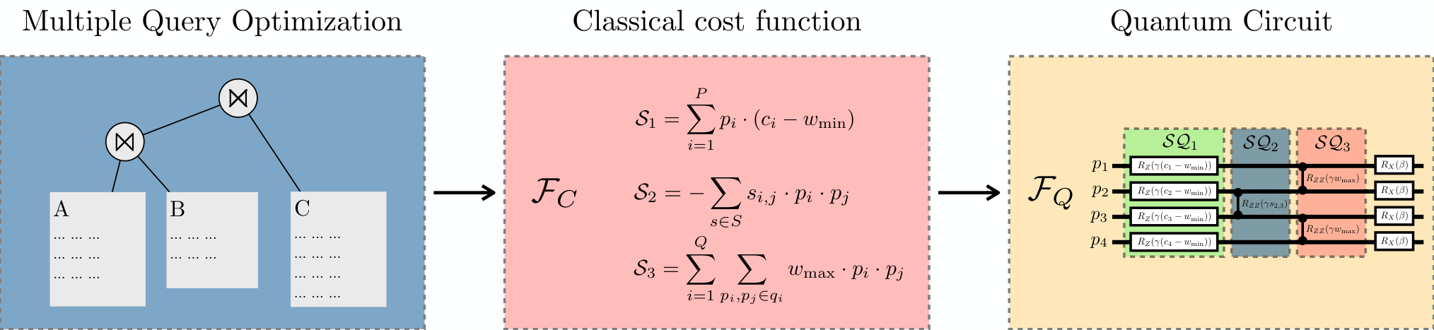
Until now, has been treated as black-box function, encoding the problem with qualitative constraints previously defined in the form of rewards and penalties. Quantitatively, the constraints can be formulated in terms of a classical cost function to be minimized, similar to [40]. To distinguish this cost function from the intuitive problem-encoding function , we subsequently call the classical cost function . The variables of the cost functions are equal to the solution-encoding bit strings (see Section 3) in the form e.g. .
For the MQO, the cost function encompasses three sums for the constraints and is defined as follows according to [40]. The sums are directly derived from the rules to defined in Section 1.
| (8) |
, and are defined as follows:
| (9) |
| (10) |
| (11) |
| (12) |
| (13) |
We will now analyze the three sums , and in more detail.
calculates the costs of all query plans . The term gives an incentive to select at least one plan. Moreover, the constant ensures that is slightly larger than the plan with the maximum cost and guarantees that at least one plan is selected for every query.
calculates the total savings of shared resources between query plans and , i.e. rewards savings if the plan pairs are selected, for which savings are applicable.
penalizes solutions that select more than one plan per query. As this is a non-negotiable constraint, it is multiplied by to dominate any bonus.
Example 3
To illustrate the cost function, we apply it on the example MQO. Recall that the costs for the plans are and - as shown previously in Example 2. When the plans and are selected, they have a cost saving of . For this example we set to 1. For all solutions, we calculate and . is a non-admissible solution, as it selects plans and , where and produce the same query .
For the solution, we calculate . Then, is calculated easily as there are no savings between the selected plans hence . Finally, , which represents the penalty due to two selected plans for the same query. The complete sum is given by .
Now, we calculate the cost for the valid and optimal solution . = (3-22) + (1-22) = -40. Because no savings apply between plans and we set . as well, because and , therefore there is no pair of for the same query whose product is 1. Thus, the sum of .
The second solution with yields a lower value than the first solution with , which is desired for minimization of the cost function. Consequently the query plan is preferred over the query plan .
As the sums and are quadratic terms (i.e. they contain the product of the two variables ), this cost function is classified as a quadratic cost function. In the literature, this class of problem is also known as Quadratic Unconstrained Binary Optimization (QUBO) [40, 16]. Problems in the QUBO formulation have a similar form to problems solvable by Quantum Computers55 5 More precisely, these are Ising models, described by Hamiltonian matrices[27]. [2, 17]. Here, we omit the quantum mechanical intricacies, but refer to [12, 30] for a more detailed explanation of this relationship.
4.3 Implementing as Quantum Circuit
On a practical level, the relation between the QUBO form of and quantum computing is due to quantum gates that typically act on one or two qubits and QUBO problems that feature one or two variables in every term. Hence, linear variables of the classical cost function are translated into two standard gates in quantum computing, a quantum rotation gate with the parameter being proportional to the scalar (such as cost) the variable is multiplied with. Quadratic variables are implemented using -gates (another standard type of gate) acting on two qubits, representing the two variables. We subsequently call the quantum-gate implementation of the classical cost function , or quantum cost function.
Example 4
To illustrate the implementation consider the example MQO. First, the linear (quantum) sum is implemented:
| (14) |
acting on the qubits that encode the plans. Note that the factor controlling the step size for gate-based quantum computer is encompassed as well. Here, this sum produces one -gate for every plan i.e. qubit. Assuming , we obtain for the first plan that has cost of and with that is the gate , where is the qubit the gate is applied to. The plans to are created in the same manner.
Quadratic sums are implemented analogously, as for instance with , which is internally quadratic:
| (15) |
This gives us a gate for every saving, which is pairwise between plans. As there is only a single saving between plans and with the value , the quantum gate is . Note that the negative sign of the sum has been taken in front of the saving’s cost as gate parameter.
Lastly, is implemented as follows:
| (16) |
This sum typically contributes the majority of gates as all plans within a query must be pairwisly connected. Recall that equals to . For query this yields the gate and for query the gate .
A general analysis of the amount of quantum gates depending on the problem size is given at the end of Section 5.
This notation is arguably cumbersome, and the encoding is better readable in the form of a quantum circuit, depicted in Figure 7. In difference to the classical cost function, an additional array of gates is necessary due to the adiabatic principle. More precisely, for each qubit encoding a plan , a single -gate (another standard gate) is appended to . The exact reasons for this requirement are beyond the scope of this work and are treated in [12, 43]. Intuitively, the -gates can be described as "driver" gates for the quantum annealing evolution66 6 Therefore, the requirement is known as driver Hamiltonian..

4.4 Running the Algorithm
The hybrid classical-quantum algorithm has two degrees of freedom. First, the number of steps is decomposed into and secondly, the number of times the circuit is run and parameters and are optimized. We subsequently refer to as depth. Currently, QAOA is in general not well understood for depths [43]. An exception to this is the recent contribution by Arute, Frank et al., examining circuits with on Google’s private Sycamore quantum device [21]. Although higher depth theoretically leads to better results, as the quantum annealing evolves "smoother" (see Fig. 4), more gates contribute to more error [12]. Hence, the depth should be chosen carefully depending on factors such as problem size or error rate of the quantum device. As each additional layer of contributes another pair of parameters and , the parameter space to be classically optimized quickly increases, as already noted by the original authors [12]. To mitigate this problem, Zhou, Wang et al. provide helpful heuristics and strategies, which they prove by extensive experimentation on graph problems [43]. We examine their contributions and their applicability to our algorithm in the next section.
The low-level hybrid algorithm for the MQO can now be summarized as follows (see Algorithm 2). In contrast to the high-level algorithm (see Algorithm 1), the MQO is first encoded as a classical cost function , which is then translated into a quantum cost function with the additional "driver" gates. As is applied in steps, parameters are used for the application of inside the quantum circuit. After has been applied on the quantum circuit, the measurement represents a solution to the MQO problem, which we denote by . The cost of can be classically evaluated as shown in Example 4.1.
The parameters are first randomly initiated, and then classically optimized by a classical computer after each measurement. The goal is to find parameters that allow to produce the bit sequence of the least-cost solution on the quantum register. This goal is reached exactly when is applied "most effectively", as introduced at the beginning of this section. For that, we minimize the quantum cost function equivalently as to minimize
| (17) |
As the algorithm is approximate, the optimization loop is typically executed until a threshold is reached instead of finding the exact solution. Often, an approximation ratio is used as figure of merit for ’s performance [12]. is defined as follows:
| (18) |
where denotes a lower bound for the cost of the MQO problem.
superposition;
register;
To summarize, the algorithm proceeds as follows:
- 1.
Formulate the MQO into a quantum cost function using a classical computer.
- 2.
Initialize parameters .
- 3.
Create superposition on quantum register, apply in steps on the quantum register.
- 4.
Measure the quantum register.
- 5.
Classically optimize with the goal of minimizing the cost of the results and repeat from (3) until threshold is reached.
Figure 8 shows the probability distribution of the output of the circuit after 1000 measurements for selected iterations of the classical optimizer. Initially the probabilities to measure any state are distributed evenly as shown in Figure 8 (a). After 14 iterations the most likely state, would represent a non-valid solution as shown in Figure 8 (b). Because the classical optimizer was able to avoid any local optima in this example, it minimizes the cost function even further and eventually approaches the right solution as most likely state to be measured - see Figure 8 (c), (d).

5 Experiments and Results
The primary objective of our experiments is to determine how the hybrid classical-quantum algorithm QAOA scales on current quantum computers, i.e. how well we can solve query optimization problems. Therefore, we compare the performance of various problem sizes, i.e. various number of queries and various numbers of query plans, with different numbers of repetitions of - the quantum part of the query optimization algorithm shown in Algorithm 2. contains the QUBO-problem to solve and adds its characteristic structure and values to the quantum circuit.
The algorithm’s "division of labor" can be summarized as follows. The parametrized quantum part explores the search space. By exploiting quantum properties such as superposition and entanglement, the exploration is typically much faster than by classical approaches. The classical part is concerned with finding parameters and that, fed to the quantum part, direct the exploration into promising regions of the search space. With growing problem search space, the parameter search space grows as well [12, 43], making the classical optimization challenging.
Therefore, we first analyze the classical part of the QAOA on the Qiskit quantum simulator [2]. In particular, we analyze what makes good and . Afterwards, we investigate the performance of different classical optimizers. The FOURIER strategy [43] is a recent suggestion to improve optimization in the high-dimensional parameter space, by using a heuristic.
Finally, we evaluate the quantum part of our hybrid classical-quantum algorithm where we run experiments on two different instances. For development and benchmarking, the quantum part of the algorithm is executed on the Qiskit quantum simulator. For experimentation and benchmarking, it is run on the publicly available ibmq Melbourne [25] device, featuring 15 qubits. This device is also used in recent research, including [33]. Our implementation can be executed on both instances without modification of the code77 7 The source code is available at: https://github.com/macemoth/QuantumQueryOptimization.
The main difference between quantum simulators and real quantum devices is that the simulators produce results without noise. This means that on a simulator, one can work without error correction. With current hardware, up to 61 qubits can be simulated using supercomputers [42], with desktop computers, quantum algorithms below 30 qubits are realistic [2]. As current quantum systems feature a comparable amount of qubits, the size of problems our algorithm can tackle is restricted by both quantum simulators and real quantum devices.
5.1 Bootstrapping the Classical Optimization Part with a FOURIER Strategy
When is constructed in Algorithm 2, initial values for parameters and need to be set to start the classical optimization. Usually those values are set randomly. Initializing and at random has multiple disadvantages. First, the randomly generated values often lead the optimizer to converge against local optima and therefore the circuit returning sub optimal solutions. Second, the more repetitions of are applied to the circuit, the more parameters need to be initialized. Hence finding good initial parameters through random initialization gets exponentially more difficult.
We base our experiments on the FOURIER heuristic strategy introduced in [43] which seems to perform very well in finding good initial parameters for and . Instead of randomly initializing and for every repetition of , the FOURIER strategy advises to calculate new values for all and through the following transformation based on previously optimized values:
where the parameters correspond to the parameters . With this strategy only the initial parameters and are determined randomly. Because of the rotational symmetry of qubit states the initial parameter guess can be restricted to . The schematic procedure for FOURIER is rendered in Figure 9.
To verify the results presented in [43] we compare the performance of the QAOA algorithm with parameters found through the FOURIER strategy against randomly initialized parameters. For the experiment we first generate a random multiple-query optimization problem of 4 qubits, i.e. 2 queries with 2 plans each. On that problem we apply the QAOA with different numbers of repetitions of . We perform 30 runs of the QAOA with FOURIER as well as with randomly initialized parameters for each number of repetitions of on the simulator. The result can be seen in Figure 10. The average FOURIER strategy performs as well as the best randomly found parameters and is therefore our algorithm of choice for determining the parameters of the further experiments.
5.2 Applying Various Classical Optimization Approaches
Classical optimization arises to be the critical part of the QAOA because of the challenge to avoid local optima. To get around this problem, we evaluate the performance of the different optimizers provided by the Qiskit library on the simulator [2]. Additionally to the classical optimizer provided by Qiskit, we also use the PennyLane library with its quantum gradient descent optimizer [2, 6]. Figure 11 shows the performance of the different optimizers with respect to the number of applications of in the circuit. All experiments are executed on the Qiskit simulator. As can be seen, for certain optimizers the quality of the solution increases with the number of repetitions as the theory suggests. Because of the steady increase and slight edge of performance of the POWELL optimizer [2], the further experiments are performed using this optimizer.
5.3 Hybrid Classical-Quantum Optimization
In this section we analyze the end-to-end query optimization problem using a hybrid classical-quantum optimization algorithm described by Algorithm 2. First we evaluate how to find the optimal parameters and , i.e. the classical part of Algorithm 2. Afterwards, we evaluate how to find the optimal number of repetitions of , i.e. the quantum part of Algorithm 2. Again, the classical part is run on the simulator while the quantum part is executed on the ibmq Melbourne quantum computer.
5.3.1 Classical Part: Finding Optimal Parameters for and
We first analyze the "classical part" of Algorithm 2, i.e. to find the optimal parameter setting of and . Note that finding the optimal parameters and appears to be the main difficulty to apply the QAOA successfully on quantum computers [12, 43, 21]. To get to the bottom of the problem, we try to determine what makes good and . Because this step happens with a classical optimizer e.g. gradient descent or other non-linear optimizers in a non-convex cost landscape, the optimizer can severely fail to find a good solution [43]. Therefore, restricting the search space to good candidates for and can drastically enhance the solution quality and the time consumed by classical optimizers.
To evaluate whether there exist patterns in good candidates, we record the parameters which lead to right solutions for different problem sizes. We expect a steady increase in value for the parameter compared to with and a decrease in value for the parameter compared to with . This behavior is predicted by the adiabatic principle and shown by [43].
Although the application of the FOURIER strategy always resets the initial parameters in a similar way, the classical optimization part finds good solutions scattered all over the search space. As can be seen in Figure 12, there is no obvious pattern in the parameter setting of and , such that the QAOA can extract the optimal solution. Hence, the optimal parameter setting must be determined empirically for each problem.
5.3.2 Quantum Part: Finding Optimal Repetitions of
Next, we analyze the "quantum part" of Algorithm 2, i.e. to find the optimal number of repetitions of depending on the size of our multiple-query optimization problem. In particular, we vary the number of queries as well as the number of query plans and study the probabilities of finding the optimal solution, i.e. the optimal query plan, for various problem sizes.
The QAOA algorithm is currently not well understood beyond repetitions of . To investigate the behavior and necessity of more than 1 repetition for larger problem sizes, we apply the QAOA on various randomly generated MQO problems up to problem sizes of 14 plans (resulting in the same number of qubits). In theory, and empirically proven on the simulator in our experiments before, more applications of should lead to a better approximation of the minimum cost but at the same time deepening the circuit and increasing the gate induced error [43, 21].
We perform this experiment on the ibmq Melbourne quantum computer where we evaluate the accuracy of the QAOA on 50 different problems on each problem size.

Figure 13 shows the probability of finding the optimal solution as a function of the number of qubits, i.e. problem size, and the number of repetitions of . We measured the results on problems of size 4 to 14 qubits and with 1 to 10 repetitions of in the circuit. Our experimental results show that for a problem size of 4 qubits, i.e. 2 queries with 2 query plans each, the probability of finding the optimal solution is 59%. For a problem size of 6 qubits, with 4 repetitions of , the optimal solution is found with a probability of 16%. For problem sizes of 8 qubits and above, the probability of finding the optimal solution converges to zero. In other words, deeper circuits can currently not be processed by the ibmq Melbourne device.
5.4 Experimental Algorithm Run Times
Each run is concluded by measuring the state of the qubits, which is a stochastic procedure. For statistics, the quantum circuit is executed and then measured multiple times, where each cycle is called a shot. Typically, thousand to ten thousand shots are conducted [20]. Table 1 shows the minimum, median and maximum run times for four differently sized problems. For all experiments, five repetitions of , that is, were used on the ibmq Melbourne device.
| Run time in ms | |||||
|---|---|---|---|---|---|
| Min. | Med. | Max. | |||
| 14 Qbits | 7 | 2 | 14.2 | 28.0 | 35.3 |
| 2 | 7 | 23.8 | 25.0 | 30.9 | |
| 7 Qbits | 4 | 2 | 14.3 | 15.1 | 15.2 |
| 2 | 4 | 14.6 | 15.2 | 15.7 | |
The run times mainly depend on the number of qubits used, which are determined by the number of plans the number of queries. If there are many alternative plans for each query (i.e. is large), the execution time increases slightly. Although the doubling of qubits used leads to doubling in run times, this correlation might be coincidental. The time complexity is analyzed in more detail at the end of this section. Generally, the execution time is not only determined by the amount of gates, but as follows: (time to prepare the qubit’s state) + (time per gate) (amount of gates) + (time to measure) [20].
5.5 Comparison with Competing Approaches
For the MQO problem [37], a variety of approaches have been suggested. Early methods were based on graphs, using algorithms based on A* and branch-and-bound techniques [18, 37]. Since then, integer linear programming [11] and genetic algorithms [5] have been proposed, improving prior methods. More recent approaches employ dynamic programming, while considering multiple cost metrics [41]. In case of the more general class of query optimization problems, learning algorithms have successfully been applied [39]. Modern approaches extend this approach with the usage of deep learning methods [28, 22].
Whilst almost all of the existing approaches rely on classical computing architecture, to the best of our knowledge, there is only one quantum-based solution to address the MQO suggested by Trummer and Koch [40]. In the following paragraph, we compare these two approaches in more detail.
In their paper, Trummer and Koch utilize a D-Wave quantum annealer with more than 1000 qubits [40], while we employ a gate-based quantum computer with 15 qubits [25]. The qubit disparity between quantum annealers and gate-based quantum computers persists to this day, with quantum annealers featuring almost two orders of magnitude more qubits than gate-based quantum computers [10, 24]. Clearly, the D-Wave device’s superiority in qubits allows it to solve larger problems with as many as 1074 queries with two plans each, or 540 queries with 5 plans each, as shown in Table 2.
| Trummer and Koch | This work | |
|---|---|---|
| Max. # of queries | 537 queries, 2 plans | 7 queries, 2 plans |
| Qubits used | 1074 / 1097 (98%) | 14 / 14 (100%) |
| Max. # of plans | 108 queries, 5 plans | 2 queries, 7 plans |
| Qubits used | 540 / 1097 (49%) | 14 / 14 (100%) |
Similarly to our approach, Trummer and Koch assign plans to qubits that are either selected or not to form the solution to the MQO. For this, they map plans as variables to the physical qubits, called physical mapping [40]. The physical layout of the qubits on the D-Wave quantum annealer is represented as Chimera graph [29] as in Figure 14.
To model cost savings, which become active when certain pairs of qubits have been selected for the solution, qubits have to interact with each other (this is, they are entangled). For this interaction, plan-encoding qubits have to be connected to each other. As the Chimera graph is not fully connected, it is necessary to encode a plan in multiple qubits to ensure that the necessary interactions can be facilitated. An example for this encoding is the TRIAD pattern (see Fig. 14) [40], where a total of eight variables are mapped to 24 qubits to become fully connected.
This mapping introduces two restrictions. First, the physical mapping introduces an overhead, in particular with problems that require strong interaction. An example of such a problem is the MQO with many plans per query. With the requirement to only choose one plan per query, all plans within that query must be connected, augmenting the degree of interaction. As a consequence, with a higher number of plans per query, around half of the quantum annealer’s qubits are required for the physical mapping, as shown in Table 2. The second restriction is that the physical mapping with the minimal number of qubits is itself an NP-hard problem [26].
Although our approach is heavily limited by the number of qubits of gate-based quantum devices, it does not suffer both of these restrictions, as all of the available qubits can be used to encode plans and the physical mapping is a one-to-one mapping from a variable to a qubit.
Both our approach on QAOA as well as quantum annealing are founded on the quantum-mechanical adiabatic principle [12, 13, 43]. In quantum annealing, the minimum spectral gap , informally described as a property of the problem-encoding function , determines how much time is required for the adiabatic evolution [43] (we use the conventions and units of this work). The relationship is given by
| (19) |
Zhou et al. [43] report that some graph-based problems ("hard problems") exhibit very small minimum spectral gaps, thus requiring a very long time to evolve, as described by the relationship above. When evolved too quickly, the quantum annealing algorithm can leave it’s "path", and thus produces a completely different result [13], as illustrated in Figure 15.
The time required to evolve would in practice render quantum annealing ineffective for those problems. Zhou et al. further report that QAOA can overcome this limitation, as it adjusts its parameters during the optimization procedure. Hence, QAOA can conclude the adiabatic evolution much faster and solve problems that can not effectively be solved by quantum annealing. This resistance makes QAOA more robust in tackling these hard problems.
Zhou et al. classify gaps as very small [43] and thus problematic for quantum annealing. Existing approaches typically compute the minimal gap for random problem instances [43] or estimate it for particular problems [13]. Farhi et al. state that they are in general unable to estimate the gap. Choi [9] examines the effects of the problem88 8 More specifically, the problem Hamiltonian. on the gap analytically. Choi notes that the relation between the problem encoding (introduced as ) and the driver gates (see Section 4.3) plays a significant role for the minimum gap. For general search problems, Albash et al. [3] indicate an inverse scaling of the minimum gap with the number of qubits (i.e. problem size), identifying the gap (-scaling) as a problem for quantum annealing. For the MQO, we numerically evaluate the minimum gap for several problem instances (see Table 3). The energy states of the example problem introduced in Section 1 are shown in Figure 16.
We observe that with a larger number of plans per query , typically increases. Even when increasing the number of qubits (this is, ), the minimum gap grows. This effect is different than reported for many problems in the literature. We suggest that the benevolent gap scaling is likely due to the MQO’s problem structure, where the amount of plans per query contributes strongly to the amount of qubits but has a positive influence on the minimum gap.
By constructing a problem with small but large , we indeed find that the minimum gap becomes smaller. Similarly to Zhou et al., we find a MQO problem instance that has a extremely small gap with plan cost of 8, 42, 49, 3 and savings , , and . We suspect that the very small gap partially stems from the large savings, and are able to reproduce this problem to some degree by introducing large savings. However, we are not able to find a pattern that routinely leads to very small gaps.
This coincides with the observations of most authors, that very small gaps are observed for special instances found at random rather than by construction. Based on the random problem instances analyzed, we suppose that there may be real MQO instances that exhibit very small minimum gaps that are indeed problematic for quantum annealers and therefore better tractable by our approach instead of quantum annealing.
| Plans | Qubits | ||
|---|---|---|---|
| # of qubits | |||
| 2 | 0.134 | 4 | 0.134 |
| 3 | 0.180 | 6 | 0.076 |
| 4 | 0.169 | 8 | 0.140 |
| 5 | 0.262 | 10 | 0.213 |
5.6 Scaling the Problem
Current quantum devices are severely limited by the number of qubits they feature. Moreover, gate-based quantum computers, as used for this work, are additionally restricted because each operation introduces non-negligible error [34, 43]. Quantum algorithms, such as Shor’s algorithm [38] assume availability of fault-tolerant quantum computers comprising millions of qubits [30]. Those computers cannot be constructed currently. In addition, algorithms designed to run on near-term quantum computers, such as QAOA [12], can currently only be used to solve very small proof-of-concept problems. Hence, solving such problems on current gate-based quantum computers gives only limited insight in the real-world use of quantum algorithms. Simulators remain to experimentally examine quantum algorithms merely beyond this insight99 9 A notable exception is Arute et al.’s experiment, claiming to outperform a classical simulation [4].. Nevertheless, it remains to analyze quantum algorithms analytically. In the next paragraph we analyze our algorithm in terms of scaling, as the intention is to devise quantum algorithms that potentially solve problems faster than classical computers.
We provide a sketch of the computational complexity of our algorithm and compare it with the classical brute-force approach introduced in Section 3. Recall that for the MQO, we denote the number of queries by , the number of plans per query by and the total number of plans by . For each of the queries, one of the plans must be selected. With this requirement, only admissible solutions remain.
| poss. | poss. | … | possibilities |
By brute force, possibilities must be evaluated1010 10 If we included non-admissible solutions with no or more than one plan per query, evaluations would be required.. Considering a constant time to evaluate the cost of each solution, the complexity of the brute force approach is as follows:
| (20) |
For the quantum approach, we focus on the quantum part and assume the complexity of the classic optimization as constant . Furthermore, we assume the complexity for formulating the MQO into a classical cost function, and into a quantum circuit to be constant.
The space complexity of the quantum circuit can trivially be answered as because our approach requires exactly one qubit for every plan of the MQO. The time complexity for quantum computations is typically determined by the depth of the quantum circuit [20]. This is because the depth indicates the longest succession of gates that must be executed sequentially. The time required for a computation to complete is obtained by multiplying the amount of operations with the average time a quantum gate requires [20].
For the complexity sketch, we split the quantum cost function into its three sums to . contains linear terms and only adds one gate to each qubit. Because these gates are executed simultaneously, the complexity is constant with .
is a quadratic sum and appends a gate for every pair of plans that, when active, save costs. Although very untypical, every plan could potentially exhibit cost savings when selected with any other plan (e.g. when there is an intermediate result that can be reused for all queries). The number of all plan pairs is then , resulting in a complexity of . Because only one plan can be selected per query, plans for the same query could never form pairs. Because of this, we consider this estimate an upper bound.
Finally, is another quadratic sum. It penalizes the selection of more than one plan per query. For this, it connects all plans inside a query with each other pairwisely by adding a gate to every pair. Similar to above, all plan pairs inside the query are , contributing to a complexity of . These gates can be applied simultaneously for all queries, therefore, the number of queries is not decisive.
As the three components of are sequentially connected, the individual complexity sketches can be added. Because is run times in the optimization loop with the classical optimizer (which is assumed here), the complexity of QAOA is
| (21) |
After reformulation, we end up with the following complexity of QAOA:
| (22) |
Compared to the brute force complexity of , this is a significant speedup. For comparison, Grover’s algorithm for searching an unstructured list achieves a speedup from to . This suggests that the quantum part of the algorithm does not only work for very small problems, but also for real-world sized problems, as the number of gates grows moderately.
Example 5
In both classical and quantum computing, the amount of operations determines the time and feasibility for a computation [31, 20]. In this example, we estimate and compare the amount of operations of the QAOA algorithm with the brute force approach for different problem sizes (see Table 4). For our quantum query optimization algorithm, we neglect the number of iterations of the optimization loop, as the same circuit is run in each iteration. Thus, the number of iterations does not determine the amount of quantum gates required.
| # of operations | ||
|---|---|---|
| Problem size | Brute Force | QAOA |
| , | ||
| , | ||
| , | ||
With larger problem instances, our algorithm requires clearly fewer operations than a brute force algorithm. Still, the two larger problem sizes could not be solved on a current gate-based quantum computer [25], and as described previously.
The complexity sketch above, however, neglects the non-trivial classical optimization procedure, which is analyzed in Zhou et al. [43] and from a more theoretical aspect in Farhi and Harrow [14]. In the same paper, Farhi and Harrow analyze the prospects of QAOA for near-term quantum devices and as candidate for a problem-solving technique superior to any classical approach. Guerreschi and Mazuura [20] argue that the necessary speedup with QAOA can be attained with hundreds of qubits. They also propose a complete estimate on the computational time of realistic QAOA applications.
6 Conclusion
In this paper we have proposed a hybrid classical-quantum algorithm based on the Quantum Approximate Optimization Algorithm to find quasi-optimal solutions for the multiple query optimization problem, a classical problem in database optimization. Our algorithm is designed for near-term gate-based quantum computers, consisting of a parametrized quantum part for exploring the search space, and a classical part optimizing the parameters. Our approach is the first contribution to use gate-based quantum computers for tackling query optimization. While the classical part of hybrid classical-quantum algorithms is typically difficult due to the high-dimensional parameter space, we implemented a recently suggested strategy as remedy, thus improving the solution quality.
As current-day gate-based quantum computers are restricted in the amount of qubits and fault-tolerance, our gate-based algorithm can currently not directly compete against implementations on a quantum annealing architecture, for which quantum devices with more capacity exist. However, when comparing our hybrid approach with a competing pure quantum-annealing approach, we found that our approach has two advantages. Firstly, it can utilize the quantum device’s qubits more efficiently, as we have a direct mapping from the mathematical formulation to the quantum implementation. In contrast, an ideal mapping with quantum annealers is an NP-complete problem. Secondly, our algorithm is based on an approach that was previously shown to solve "hard" problems that quantum annealers may not be able to solve and that may be found within the MQO context.
Finally, we analytically sketched the scaling of our algorithm and found that with larger problem sizes, the computational time grows polynomially while the solution space grows exponentially. Further, the space requirements only grow linearly with the problem size.
We believe that our paper lays a solid groundwork for using hybrid classical-quantum algorithms to tackle the special problem of database optimizations as well as the generic class of binary optimization problems.
References
- [1] Scott Aaronson. Quantum computing since Democritus. Cambridge University Press, 2013.
- [2] Héctor Abraham, AduOffei, Rochisha Agarwal, Ismail Yunus Akhalwaya, Gadi Aleksandrowicz, Thomas Alexander, and Matthew Amy. Qiskit: An open-source framework for quantum computing, 2019.
- [3] Tameem Albash and Daniel A Lidar. Adiabatic quantum computation. Reviews of Modern Physics, 90(1):015002, 2018.
- [4] Frank Arute, Kunal Arya, Ryan Babbush, Dave Bacon, Joseph C. Bardin, Rami Barends, Rupak Biswas, Sergio Boixo, Fernando G. S. L. Brandao, David A. Buell, Brian Burkett, Yu Chen, Zijun Chen, Ben Chiaro, Roberto Collins, William Courtney, Andrew Dunsworth, Edward Farhi, Brooks Foxen, Austin Fowler, Craig Gidney, Marissa Giustina, Rob Graff, Keith Guerin, Steve Habegger, Matthew P. Harrigan, Michael J. Hartmann, Alan Ho, Markus Hoffmann, Trent Huang, Travis S. Humble, Sergei V. Isakov, Evan Jeffrey, Zhang Jiang, Dvir Kafri, Kostyantyn Kechedzhi, Julian Kelly, Paul V. Klimov, Sergey Knysh, Alexander Korotkov, Fedor Kostritsa, David Landhuis, Mike Lindmark, Erik Lucero, Dmitry Lyakh, Salvatore Mandrà, Jarrod R. McClean, Matthew McEwen, Anthony Megrant, Xiao Mi, Kristel Michielsen, Masoud Mohseni, Josh Mutus, Ofer Naaman, Matthew Neeley, Charles Neill, Murphy Yuezhen Niu, Eric Ostby, Andre Petukhov, John C. Platt, Chris Quintana, Eleanor G. Rieffel, Pedram Roushan, Nicholas C. Rubin, Daniel Sank, Kevin J. Satzinger, Vadim Smelyanskiy, Kevin J. Sung, Matthew D. Trevithick, Amit Vainsencher, Benjamin Villalonga, Theodore White, Z. Jamie Yao, Ping Yeh, Adam Zalcman, Hartmut Neven, and John M. Martinis. Quantum supremacy using a programmable superconducting processor. Nature, 574(7779):505–510, 2019.
- [5] Murat Ali Bayir, Ismail H Toroslu, and Ahmet Cosar. Genetic algorithm for the multiple-query optimization problem. IEEE Transactions on Systems, Man, and Cybernetics, Part C (Applications and Reviews), 37(1):147–153, 2006.
- [6] Ville Bergholm, Josh Izaac, Maria Schuld, Christian Gogolin, M Sohaib Alam, Shahnawaz Ahmed, Juan Miguel Arrazola, Carsten Blank, Alain Delgado, Soran Jahangiri, et al. Pennylane: Automatic differentiation of hybrid quantum-classical computations. arXiv preprint arXiv:1811.04968, 2018.
- [7] Max Born and Vladimir Fock. Beweis des adiabatensatzes. Zeitschrift für Physik, 51(3-4):165–180, 1928.
- [8] Nikhil Buduma and Nicholas Locascio. Fundamentals of deep learning: Designing next-generation machine intelligence algorithms. " O’Reilly Media, Inc.", 2017.
- [9] Vicky Choi. The effects of the problem hamiltonian parameters on the minimum spectral gap in adiabatic quantum optimization. Quantum Information Processing, 19(3):1–25, 2020.
- [10] D-Wave Systems Inc. A the d-wave 2000qtm quantum computer technology overview, 2017. Accessed 08.06.2021.
- [11] Tansel Dokeroglu, Murat Ali Bayır, and Ahmet Cosar. Integer linear programming solution for the multiple query optimization problem. In Information Sciences and Systems 2014, pages 51–60. Springer, 2014.
- [12] Edward Farhi, Jeffrey Goldstone, and Sam Gutmann. A quantum approximate optimization algorithm. arXiv preprint arXiv:1411.4028, 2014.
- [13] Edward Farhi, Jeffrey Goldstone, Sam Gutmann, and Michael Sipser. Quantum computation by adiabatic evolution. arXiv preprint quant-ph/0001106, 2000.
- [14] Edward Farhi and Aram W Harrow. Quantum supremacy through the quantum approximate optimization algorithm, 2019.
- [15] Richard P Feynman. Simulating physics with computers. Int. J. Theor. Phys, 21(6/7), 1982.
- [16] Austin Gilliam, Stefan Woerner, and Constantin Gonciulea. Grover adaptive search for constrained polynomial binary optimization. Quantum, 5:428, 2021.
- [17] Fred Glover, Gary Kochenberger, and Yu Du. A tutorial on formulating and using qubo models, 2019.
- [18] John Grant and Jack Minker. On optimizing the evaluation of a set of expressions. International Journal of Computer & Information Sciences, 11(3):179–191, 1982.
- [19] Lov K Grover. A fast quantum mechanical algorithm for database search. In Proceedings of the twenty-eighth annual ACM symposium on Theory of computing, pages 212–219, 1996.
- [20] Gian Giacomo Guerreschi and Anne Y Matsuura. Qaoa for max-cut requires hundreds of qubits for quantum speed-up. Scientific reports, 9(1):1–7, 2019.
- [21] Matthew P. Harrigan, Kevin J. Sung, Matthew Neeley, Kevin J. Satzinger, Frank Arute, Kunal Arya, Juan Atalaya, Joseph C. Bardin, Rami Barends, Sergio Boixo, Michael Broughton, Bob B. Buckley, David A. Buell, Brian Burkett, Nicholas Bushnell, Yu Chen, Zijun Chen, Ben Chiaro, Roberto Collins, William Courtney, Sean Demura, Andrew Dunsworth, Daniel Eppens, Austin Fowler, Brooks Foxen, Craig Gidney, Marissa Giustina, Rob Graff, Steve Habegger, Alan Ho, Sabrina Hong, Trent Huang, L. B. Ioffe, Sergei V. Isakov, Evan Jeffrey, Zhang Jiang, Cody Jones, Dir Kafri, Kostyantyn Kechedzhi, Julian Kelly, Seon Kim, Paul V. Klimov, Alexander N. Korotkov, Fedor Kostritsa, David Landhuis, Pavel Laptev, Mike Lindmark, Martin Leib, Orion Martin, John M. Martinis, Jarrod R. McClean, Matt McEwen, Anthony Megrant, Xiao Mi, Masoud Mohseni, Wojciech Mruczkiewicz, Josh Mutus, Ofer Naaman, Charles Neill, Florian Neukart, Murphy Yuezhen Niu, Thomas E. O’Brien, Bryan O’Gorman, Eric Ostby, Andre Petukhov, Harald Putterman, Chris Quintana, Pedram Roushan, Nicholas C. Rubin, Daniel Sank, Andrea Skolik, Vadim Smelyanskiy, Doug Strain, Michael Streif, Marco Szalay, Amit Vainsencher, Theodore White, Z. Jamie Yao, Ping Yeh, Adam Zalcman, Leo Zhou, Hartmut Neven, Dave Bacon, Erik Lucero, Edward Farhi, and Ryan Babbush. Quantum approximate optimization of non-planar graph problems on a planar superconducting processor, 2021.
- [22] Jonas Heitz and Kurt Stockinger. Join query optimization with deep reinforcement learning algorithms. arXiv preprint arXiv:1911.11689, 2019.
- [23] Matthias Homeister. Quantum Computing verstehen. Springer, 2008.
- [24] IBM Quantum team. ibmq_manhattan v1.21.0, 2021. Accessed 09.06.2021.
- [25] IBM Quantum team. ibmq_melbourne v2.3.24, 2021. Accessed 02.06.2021.
- [26] Christine Klymko, Blair D Sullivan, and Travis S Humble. Adiabatic quantum programming: minor embedding with hard faults. Quantum information processing, 13(3):709–729, 2014.
- [27] Andrew Lucas. Ising formulations of many np problems. Frontiers in Physics, 2:5, 2014.
- [28] Ryan Marcus, Parimarjan Negi, Hongzi Mao, Chi Zhang, Mohammad Alizadeh, Tim Kraska, Olga Papaemmanouil, and Nesime Tatbul. Neo: A learned query optimizer. arXiv preprint arXiv:1904.03711, 2019.
- [29] Catherine C McGeoch and Cong Wang. Experimental evaluation of an adiabiatic quantum system for combinatorial optimization. In Proceedings of the ACM International Conference on Computing Frontiers, pages 1–11, 2013.
- [30] Nikolaj Moll, Panagiotis Barkoutsos, Lev S Bishop, Jerry M Chow, Andrew Cross, Daniel J Egger, Stefan Filipp, Andreas Fuhrer, Jay M Gambetta, Marc Ganzhorn, et al. Quantum optimization using variational algorithms on near-term quantum devices. Quantum Science and Technology, 3(3):030503, 2018.
- [31] Michael A Nielsen and Isaac Chuang. Quantum computation and quantum information, 2002.
- [32] Alberto Peruzzo, Jarrod McClean, Peter Shadbolt, Man-Hong Yung, Xiao-Qi Zhou, Peter J Love, Alán Aspuru-Guzik, and Jeremy L O’brien. A variational eigenvalue solver on a photonic quantum processor. Nature communications, 5(1):1–7, 2014.
- [33] Christophe Piveteau, David Sutter, and Stefan Woerner. Quasiprobability decompositions with reduced sampling overhead, 2021.
- [34] Timothy Proctor, Kenneth Rudinger, Kevin Young, Erik Nielsen, and Robin Blume-Kohout. Demonstrating scalable benchmarking of quantum computers. Bulletin of the American Physical Society, 65, 2020.
- [35] P Griffiths Selinger, Morton M Astrahan, Donald D Chamberlin, Raymond A Lorie, and Thomas G Price. Access path selection in a relational database management system. In Readings in Artificial Intelligence and Databases, pages 511–522. Elsevier, 1989.
- [36] Timos Sellis and Subrata Ghosh. On the multiple-query optimization problem. Knowledge and Data Engineering, IEEE Transactions on, 2:262 – 266, 07 1990.
- [37] Timos K Sellis. Multiple-query optimization. ACM Transactions on Database Systems (TODS), 13(1):23–52, 1988.
- [38] Peter W Shor. Polynomial-time algorithms for prime factorization and discrete logarithms on a quantum computer. SIAM review, 41(2):303–332, 1999.
- [39] Michael Stillger, Guy M Lohman, Volker Markl, and Mokhtar Kandil. Leo-db2’s learning optimizer. In VLDB, volume 1, pages 19–28, 2001.
- [40] Immanuel Trummer and Christoph Koch. Multiple query optimization on the d-wave 2x adiabatic quantum computer. arXiv preprint arXiv:1510.06437, 2015.
- [41] Immanuel Trummer and Christoph Koch. Multi-objective parametric query optimization. ACM SIGMOD Record, 45(1):24–31, 2016.
- [42] Xin-Chuan Wu, Sheng Di, Emma Maitreyee Dasgupta, Franck Cappello, Hal Finkel, Yuri Alexeev, and Frederic T. Chong. Full-state quantum circuit simulation by using data compression. In Proceedings of the International Conference for High Performance Computing, Networking, Storage and Analysis, SC ’19, New York, NY, USA, 2019. Association for Computing Machinery.
- [43] Leo Zhou, Sheng-Tao Wang, Soonwon Choi, Hannes Pichler, and Mikhail D Lukin. Quantum approximate optimization algorithm: Performance, mechanism, and implementation on near-term devices. Physical Review X, 10(2):021067, 2020.