Entanglement and charge-sharpening transitions in U(1) symmetric monitored quantum circuits

Following Khemani et al. 2018, we consider a one-dimensional chain in which each site hosts a two-level system (“qubit”) and a $d$-level system (“qudit”), i.e., the on-site Hilbert space is $\mathbb{C}^{2}\otimes\mathbb{C}^{d}$ for $d>1$ and $\mathbb{C}^{2}$ for $d=1$. The dynamics will consist of local unitary gates and measurements, which are chosen to conserve the U(1) charge

is acting on the $i$th site of the chain of length $L$ and $\mathbb{I}$ is the identity matrix on the qudits. These chains evolve under (i) unitary two-qubit gates, acting on nearest neighbor sites, which conserve the global charge $\mathcal{Q}$, and (ii) single-site projective measurements in which the qubit is measured in its $Z$ basis and the qudit is simultaneously measured in some reference basis ¹¹ 1 Since the unitaries acting on the qudits are random, the randomizing measurement basis is superfluous.. At each time-step, a given site is measured with probability $p$; for specificity, we assume that when this happens both the qubit and the qudit are measured, so the measurement acts on that site as a rank-1 projector. The symmetry-preserving two-site unitary gates are arranged in a brickwork geometry and take the form

where $i$ labels a site, $U^{\mathfrak{q}}_{D\times D}$ is a unitary matrix of size $D\times D$ acting on the charge $\mathfrak{q}_{1}+\mathfrak{q}_{2}=\mathfrak{q}\in\{0,1,2\}$ sector (a local charge is defined to take values $0$ and $1$), and $D$ is the dimension of the Hilbert space of the charge sector. Each matrix is drawn independently from the Haar random ensemble of unitary matrices of the appropriate size.

We present numerical results for this class of circuits in two limits. First, we consider the limit $d=1$, where there is no qudit degree of freedom, and one simply has a chain of qubits interacting via gates that conserve the charge $\mathcal{Q}$. In this limit, we obtain numerical results by direct time evolution. Second, we consider the complementary limit $d=\infty$, in which we can map the problem to a statistical mechanics model and explicitly write down a transfer matrix that generates the observables of interest. The phase diagrams in the two complementary limits are similar.

The qubit-only ($d=1$) model is directly realizable in existing quantum processors. The $d>1$ model is perhaps less natural experimentally, but could be realized in circuit quantum electrodynamics setups Blais et al. 2021 in which superconducting transmon qubits are coupled to multilevel superconducting cavities (qudits), or by blocking multiple qubits together (e.g. $d=2$ could be realized as a two-leg ladder of qubits). Regardless of experimental implementation, we expect the $d>1$ models to capture the generic universal behavior of phases and transitions, while allowing greater theoretical control in the large-$d$ limit.

For a given choice of unitary gates and measurement locations $\mathbf{X}$ (in spacetime), the unitary-measurement dynamics can be described in terms of quantum trajectories $\rho_{\mathbf{m}}(t)=K_{\mathbf{m}}\rho K_{\mathbf{m}}^{\dagger}$. Here $\mathbf{m}$ denotes a “quantum trajectory”, associated with a fixed configuration of measurement locations $\mathbf{X}$, and measurement outcomes ${\cal M}(\mathbf{X})$. We will write $\mathbf{m}=\{\mathbf{X},{\cal M}(\mathbf{X})\}$. The Kraus operators $K_{\mathbf{m}}$ consist of random unitary gates and projection operators onto the measurement outcomes ${\cal M}(\mathbf{X})$, and we have $\sum_{\{{\cal M}(\mathbf{X})\}}K_{\mathbf{m}}^{\dagger}K_{\mathbf{m}}=\mathbb{I}$.

We will be concerned with general properties of the single-trajectory state $\rho_{\mathbf{m}}\equiv K_{\mathbf{m}}\rho K_{\mathbf{m}}^{\dagger}$. (As a concrete example, consider the purity $\Pi_{\mathbf{m}}=\mathrm{Tr}(\rho_{\mathbf{m}}^{2})/(\mathrm{Tr}\rho_{\mathbf{m}})^{2}$.) We then average over quantum trajectories, weighting each set of measurement outcomes by its probability of occurrence, i.e., the Born probability $p_{\mathbf{m}}=\mathrm{Tr}(\rho_{\mathbf{m}})$. Finally, we average the answers across the ensemble of quantum circuits.

A few comments are in order here.

1. 1.

   For an initially pure state $|\psi\rangle$ the Born probability takes the familiar form $p_{\mathbf{m}}=\|K_{\mathbf{m}}|\psi\rangle\|^{2}$, i.e., it is just the norm of the projected state. For a series of measurements interspersed with unitary gates, one can pick each measurement outcome based on the Born probability or equivalently apply a set of projectors at random and evaluate the probability of the entire measurement history by computing the norm of the state at the end of the trajectory.

2. 2.

   There are four different types of average that we will consider here: (i) the quantum expectation value of an observable $A$ in a single trajectory $\rho_{\mathbf{m}}$, namely $\mathrm{Tr}(A\rho_{\mathbf{m}})/\mathrm{Tr}\rho_{\mathbf{m}}$, which we will write as $\langle A\rangle_{\mathbf{m}}$; (ii) the (Born-weighted) average of a single-trajectory function, such as purity or entanglement entropy, over quantum trajectories (measurement outcomes); (iii) the average over unitary gates, chosen with Haar measure; and (iv) the average over spacetime points where the measurements occur (measurement locations). In much of this work, we will present results for which averages (ii)-(iv) have been done. We will use the notation $[\cdot]$ for this full average. At some points it will be useful to separate these averages. In these cases we will use the explicit notations $\sum_{\{{\cal M}(\mathbf{X})\}}(\cdot)$, $\mathbb{E}_{U}(\cdot)$, and $\mathbb{E}_{\mathbf{X}}(\cdot)$ for averages over measurement outcomes, gates, and measurement locations respectively. We will also use a shorthand notation $\mathbb{E}_{\mathbf{m}}\equiv\sum_{\mathbf{m}}p_{\mathbf{m}}(\dots)$ to denote summation over all possible measurement locations $\mathbf{X}$ including appropriate probability factors of $p$ and $1-p$, and over all measurement outcomes ${\cal M}(\mathbf{X})$, including the associated Born probability factor $p_{\mathbf{m}}$.

3. 3.

   It is crucial that the quantities of interest to us are nonlinear functions of $\rho_{\mathbf{m}}$ Skinner et al. 2019, such as $\Pi_{\mathbf{m}}$. To see the significance of this, let us compare the quantity $\Pi_{\mathbf{m}}$ to that of some simple expectation value. In $\rho_{\mathbf{m}}$, the expectation value of a local operator $A$ would be $\mathrm{Tr}(A\rho_{\mathbf{m}})/\mathrm{Tr}\rho_{\mathbf{m}}$. Averaging this over trajectories (measurement outcomes) with the Born probabilities would simply give infinite temperature behavior ²² 2 The ensemble-averaged $\rho(t)$ resulting from maximally-random, local, open-systems dynamics is indistinguishable from an infinite temperature state over distances $\sim t$.: $\sum_{\{{\cal M}(\mathbf{X})\}}(p_{\mathbf{m}}\langle A\rangle_{\mathbf{m}})=\sum_{\{{\cal M}(\mathbf{X})\}}\mathrm{Tr}(A\rho_{\mathbf{m}})=\mathrm{Tr}(A\rho(t)){\approx\mathrm{Tr}(A)/\mathrm{Tr}(1)}$, where $\rho(t)=\sum_{\{{\cal M}(\mathbf{X})\}}K_{\mathbf{m}}\rho K_{\mathbf{m}}^{\dagger}$ describes the dynamics of the density matrix in the case where the environment does not monitor or keep track of the measurement outcomes. By contrast, $\sum_{\{{\cal M}(\mathbf{X})\}}\Pi_{\mathbf{m}}p_{\mathbf{m}}=\sum_{\{{\cal M}(\mathbf{X})\}}\mathrm{Tr}(\rho_{\mathbf{m}}^{2})/\mathrm{Tr}\rho_{\mathbf{m}}$, which cannot simply be written in terms of $\rho(t)$. The averaged density matrix $\rho(t)$ is blind to measurement transitions; only nonlinear functions of single-trajectory wavefunctions detect it.

In the following, we unveil a charge sharpening transition that takes place before the entanglement transition in two distinct models of monitored U$(1)$ symmetric random quantum circuits. Our main results are summarized in Fig. 1 and discussed in more detail below.

We begin by locating the entanglement transition point $p_{c}$ in this model. In order to probe the location of the critical point and the correlation length critical exponent, we study two quantities that have been identified as good measures of the transition: the tripartite mutual information Zabalo et al. 2020 and an order parameter defined through the use of an ancilla Gullans and Huse 2020b that is coupled to one charge-$\mathcal{Q}$ sector. In the following it is essential that we use an accurate estimate of $p_{c}$ to be able to numerically disentangle it from the charge sharpening transition at $p_{\#}$.

First, the tripartite mutual information for the Rényi index $n$ is defined as

where we have chosen regions $A,B,\mbox{and }C$ to be adjacent regions of size $L/4$ and $S_{n}(A)$ is the Rényi entropy defined in Eq. (1). For $\mathcal{I}_{3,n}$ at late times ($t=4L$) we apply the finite size scaling hypothesis $\mathcal{I}_{3,n}\sim f(L^{1/\nu}(p-p_{c})),$ to locate the critical point, where $f(x)$ is a scaling function and $\nu$ is the correlation length exponent. The data for $n=1$ is shown in Fig. 2(a) where we find the data collapses with the minimum $\chi^{2}$ for the choice of $p_{c}=0.105(3)$ and $\nu=1.32(6)$. The error bars are estimated by a region in parameter space near the minimum such that $\chi^{2}<1.3\chi^{2}_{\mathrm{min}}$ Zabalo et al. 2020, see Fig 5. A similar analysis can be performed for the other Rényi entropies and the resulting values of $p_{c}$ and $\nu$ are similar for all $n\geq 1$ investigated, we find $p_{c}=0.103(4),0.12(2),0.12(1)$ and $\nu=1.37(8),1.47(3),1.5(2)$ for $n=2,5,\infty$, respectively.

At the critical point, the bipartite entanglement entropy shows a logarithmic dependence on the system size and the coefficient of the logarithmic divergence shows strong Rényi index dependence (Fig. 2(c)). This behavior can be described by

Apart from the small offset, this Rényi index dependence matches the result one expects for the ground state of a CFT Calabrese and Cardy 2009, $\alpha_{\mathrm{CFT}}(n)=\frac{c}{6}\left(1+\frac{1}{n}\right)$. The coefficients in Eq. (9) clearly differ from those at the measurement induced transition without a conservation law Zabalo et al. 2020.

As an alternative way of locating the entanglement transition, we also study the “order parameter” Gullans and Huse 2020b. In order to have the ancilla couple to the system within a particular global charge sector, we consider the qubits at two adjacent sites $i$ and $i+1$ to be in the entangled state with an ancilla: $|\Psi_{0}\rangle=\frac{1}{\sqrt{2}}(\ket{\uparrow\downarrow}\ket{1}+\ket{\downarrow\uparrow}\ket{0})$ where the ancilla has orthogonal basis states $\ket{1}$ or $\ket{0}$. We then evolve the system in time $t=2L$ without measurements in order to create a state $\ket{\Psi}=\frac{1}{\sqrt{2}}(\ket{\psi_{1}}\ket{1}+\ket{\psi_{0}}\ket{0})$ where $\ket{\psi_{0,1}}$ are orthogonal and in the same charge sector. We then run the circuit with measurements for an additional time $2L$ and compute the von Neumann entropy of the ancilla, which we denote as $S_{1,E}$ (as it probes the entanglement transition).

The results for the von Neumann entanglement entropy of the ancilla $S_{1,E}$ are shown in Fig. 2(b), and are consistent with $\mathcal{I}_{3,n}$ data: From the scaling ansatz $S_{1,E}\sim f_{E}((p-p_{c})L^{1/\nu})$, where $f_{E}(x)$ is a universal scaling function, we obtain $p_{c}=0.110(3)$ and $\nu=1.4(2)$ in good agreement with $\mathcal{I}_{3}$.

Summarizing these results, the entanglement transition in U(1)-symmetric circuits has a critical exponent $\nu$ that is consistent with the value for Haar-random circuits with no symmetries, although the nonuniversal $p_{c}$ has drifted down from the Haar value $p^{\mathrm{Haar}}_{c}\approx 0.17$ (as one might expect since each gate cannot generate as much entanglement). At $p=p_{c}$ we extract the dynamical exponent of the entanglement transition using the scaling ansatz $[S_{1,E}]\sim g_{E}(t/L^{z})$, which shows a good quality as seen in Fig. 4 for $z=1$ and $g_{E}(x)$ some universal scaling function. Again, this result is consistent with the non-conserving case. While we have focused on $\mathcal{Q}=L/2$ we have checked that for the largest system sizes considered $p_{c}$ is only very weakly affected for $\mathcal{Q}=L/2-1$ (not shown).

We now turn to estimating $p_{\#}$ in two ways: the charge variance of a state and the entropy of an ancilla entangled with two different number sectors.

First, we compute the variance of the total charge (Eqs. (2) and (4)). For a trajectory that lies in a well defined charge sector, $\delta{\cal Q}^{2}=0$, otherwise $\delta{\cal Q}^{2}\neq 0$. Therefore, we start with a pure initial state that is spread out over all of the different $\mathcal{Q}$-sectors, $|\psi_{0}\rangle=\bigotimes_{i=1}^{L}\frac{1}{\sqrt{2}}\left(\ket{\uparrow}_{i}+\ket{\downarrow}_{i}\right)$, and run the conserving hybrid dynamics to late times to determine if the system has sharpened into a single charge sector for some measurement probability $0\leq p_{\#}\leq p_{c}$, where $p_{c}\approx 0.11$ is the critical point of the entanglement transition. In this situation, the critical point of the charge sector transition can be determined by the studying the probability, $P(\delta{\cal Q}^{2}=0)$. (Recall that $\delta\mathcal{Q}^{2}$ is a quantum uncertainty that is a property of each trajectory; the probability distribution $P(\delta\mathcal{Q}^{2})$ is over trajectories and circuits, where each trajectory is weighted by its Born probability.) For large systems, $P(\delta{\cal Q}^{2}=0)\rightarrow 0$ when the system is distributed over multiple sectors while $P(\delta{\cal Q}^{2}=0)\rightarrow 1$ when the system has been constrained to a single sector. In Fig. 3(a), the fraction $N_{0}$ of trajectories having a variance $x=\delta{\cal Q}^{2}\leq s$ (with $s=10^{-2}$) is shown for various system sizes and measurement probabilities. The critical point can be identified by the crossing near $p=0.1$. Performing a finite size scaling analysis, we find the data for different system sizes collapses onto a universal curve for the critical point $p_{\#}=0.094(3)$ and correlation length exponent $\nu_{\#}=2.0(3)$.

Lastly, we consider an ancilla coupled to two different charge sectors, in particular we take $\ket{\Psi}=\ket{\psi_{\mathcal{Q}}}\ket{0}+\ket{\psi_{\mathcal{Q}-1}}\ket{1}$ where $\ket{\psi_{\mathcal{Q}}}$ represents states within the charge sector $\mathcal{Q}$ (while $\ket{1}$ and $\ket{0}$ are states of the ancilla as before). Since there is no unitary that mixes these sectors, we can say definitively that the reduced density matrix has the form

This formulation is convenient for the numerical algorithm we have developed that conserves charge since if the ancilla were just considered an extra qubit, $\ket{\Psi}$ would be in the conserving sector $M$ for $L+1$ qubits. Doing this, we compute the von Neumann entanglement entropy of the ancilla qubit that we denote as $S_{1,\mathcal{Q}}$, that is shown in Fig. 3(b). Based on the crossing in the data and the ansatz $S_{1,\mathcal{Q}}\sim g_{\mathcal{Q}}((p-p_{\#})L^{1/\nu_{\#}})$ we obtain $p_{\#}=0.088(3)$ and $\nu_{\#}=2.2(2)$, which matches the $p_{\#}$ and $\nu_{\#}$ found by $P(\delta{\cal Q}^{2}=0)$. In addition, we extract the charge sharpening transition from the probability that the ancilla has fully disentangled from the circuit by computing the fraction of trajectories $N_{\mathrm{pure}}$ that have fully purified the ancilla [Fig. 3(c)]. From the crossing of $N_{\mathrm{pure}}$ we find a third consistent estimate of $p_{\#}$ and $\nu_{\#}$. Thus, we have identified the charge sharpening transition across all sectors of $\mathcal{Q}$ with the transition in $S_{1,\mathcal{Q}}$ across $\mathcal{Q}=L/2,L/2-1$. The dynamical exponent of the charge sharpening transition is also $z=1$, as $[S_{1,\mathcal{Q}}]\sim g_{\mathcal{Q}}(t/L)$ at criticality (Fig. 4).

The two critical points we have identified in this model at $p_{\#}$ and $p_{c}$ are at least $\sim 3.5$ error bars from each other, providing evidence that a charge sharpening transition occurs before full purification. This is further exemplified by the estimated confidence intervals for the two transitions for the various probes we have considered as shown in Fig. 5. Moreover, the correlation length exponent for charge-sharpening quantities is distinct from that of the entanglement purification transition, further suggesting that these represent distinct critical points with different universality classes.

We note, however, that the close proximity of the putative two transitions make them challenging to cleanly separate numerically in small scale systems, and acknowledge that this data could in principle be accounted for by large, systematic finite-size errors in the critical exponents that affected the charge and entanglement properties differently⁶⁶ 6 In the absence of a conservation law, it has been shown that the probes we have used for the entanglement transition ($\mathcal{I}_{3,n}$ and $[S_{1,E}]$) have weak finite size drifts in Clifford circuits Zabalo et al. 2020 by examining small and large system sizes.. In the following sections, we will see that for the model with large-$d$ qudits, the location of the two transitions become clearly distinct.

We briefly review the mapping for random monitored circuits without symmetries to a statistical model Jian et al. 2020a; Bao et al. 2020. We focus on the details required for our subsequent discussion, in particular on the large dimension limit $d\rightarrow\infty$. To calculate Eq. (14) we need to average over $Q$ copies of the circuit over Haar gates and measurement outcomes (but not over measurement locations). Since the random Haar gates are drawn independently, we can individually average $Q$ copies of each gate. The combinatorial results of the averaging can be captured as a partition function that can be computed as follows: each unitary gate in the circuit is replaced by a vertex associated with a pair of permutation “spins” $\sigma_{a},\bar{\sigma}_{a}$, each belonging to the permutation group $\mathcal{S}_{Q}$. In the $d\rightarrow\infty$ limit, these spins become locked together in a single $\mathcal{S}_{Q}$ degree of freedom, $\sigma_{a}$. Vertices from adjacent gates, i.e. those which share an input/output qubit, are connected by links. The weight associated with a vertex in the partition function is given by $V_{a}=1/d^{2Q}$. The weight of the links connecting vertices with elements $\sigma_{a,b}$ is given by

where $|\sigma^{-1}_{b}\sigma_{a}|$ is equal to the number of cycles in the cycle decomposition of $\sigma^{-1}_{a}\sigma_{b}=C_{1}...C_{|\sigma^{-1}_{b}\sigma_{a}|}$. Note that the above weights are symmetric under left and right multiplication by elements of $\mathcal{S}_{Q}$.

We see that in this $d\to\infty$ limit, spins (permutations) connected by unmeasured links are forced to be the same, whereas spins on measured links are effectively decoupled, i.e. a measurements “break” the links connecting spins, diluting the lattice. This naturally yields a picture of the purification transition in terms of classical percolation of clusters of aligned permutation “spins” Skinner et al. 2019; Jian et al. 2020a; Bao et al. 2020, though of course this simple percolation picture is special to $d\rightarrow\infty$: $1/d$ fluctuations are a relevant perturbation to the percolation critical point such that finite $d$ transitions are described by a distinct universality class from percolation Jian et al. 2020a; Zabalo et al. 2022.

As we saw in Eq. (13), the calculation of $S_{n}$ requires taking the difference between two partition functions of the model described above but with different boundary condition (see Fig. 11); in the replica limit, this difference in partition functions becomes equivalent to a difference in free energies $F_{A,\emptyset}=-\log Z_{A,\emptyset}$ (since the partition functions approach unity in the replica limit). The boundary condition for the calculation of $Z_{A}$ forces a different boundary condition in region $A$, and thus introduces a domain wall (DW) near the top boundary. In the limit $d\to\infty$, the DW is forced to follow a minimal cut, defined as a path cutting a minimum number of unmeasured links (assumed to be unique for simplicity ⁷⁷ 7 DWs are restricted by unitarity to only make certain “turns” (See Zhou and Nahum 2019 for details). E.g, for $p=0$, this leads to a unique DW where the DW follows a “light cone”. For $p>0$ one can still have many degenerate paths  Li and Fisher 2021.). This can be seen as follows: due to the boundary condition in $Z_{\emptyset}$, all vertex elements in $Z_{\emptyset}$ are equal⁸⁸ 8 Any difference in the vertex elements will lead to the creation of DW which are suppressed as ${\cal O}(1/d)$ and whose contribution goes to zero as $d\rightarrow\infty$., and $Z_{\emptyset}=d^{(1-Q)N_{m}}$, where $N_{m}$ is the number of measured sites. $Z_{A}$ would be same as $Z_{\emptyset}$ except for the fact that due to the DW some links contribute different weights to $Z_{A}$. More precisely, we have $Z_{A}=d^{(k+1-Q)\ell_{\rm DW}}Z_{\emptyset}$, where $\ell_{\rm DW}=\ell_{\rm DW}(\mathbf{X})$ is equal to the number of unmeasured links that the DW crosses. Since $k+1-Q=(1-n)k<0$ for $n>1$, the DW will follow the path that minimizes $\ell_{\rm DW}$ ⁹⁹ 9 Note that the DW permutation element $(1...n)^{\otimes k}$ has $k+1$ cycles and each cycle can follow an independent path (to the leading order) Zhou and Nahum 2019. However, this subtlety will not change the final result about the minimal cut, but only leads to fluctuations contributing sub-leading logarithmic corrections (for $p>0$).. Using the expression of $Z_{A,\emptyset}$ in Eq. (13) and taking the replica limit $k\to 0$, we find $S_{n}=\ell_{\rm DW}(\mathbf{X})\ln d$, which is valid for each configuration of measurement locations. Averaging over measurement locations, we have

where $\mathbf{X}$ denotes a configuration of measurement locations (measurement outcomes and Haar gates have been averaged over to get the statistical model). In the language of the statistical model, $\mathbf{X}$ denotes a percolation configuration. $\ell_{\rm DW}$ is the length of the minimal cut from one end of the sub system $A$ to the other end.

In the $d\to\infty$ limit, equation (16) is valid for any measurement probability, $p$ ¹⁰¹⁰ 10 Note that this description of the $d\to\infty$ differs from that of Ref. Jian et al. 2020a. There the measurement locations $\sum_{\mathbf{X}}$ were averaged over directly in the partition function, in an annealed way, while we chose here to keep the measurement locations as quenched disorder. Our approach predicts a minimal cut picture consistent with Ref. Skinner et al. 2019. We leave a discussion of the validity of the replica trick in this limit to future work. . For $p=0$, there are no measured links and hence $\ell_{\rm DW}=|A|$, where $|A|$ is the length of subsystem $A$. In fact, $\ell_{\rm DW}$ undergoes a percolation transition at $p_{c}=1/2$, where $\ell_{\rm DW}$ is extensive in $|A|$ for $p<1/2$, and becomes ${\cal O}(1)$ for $p>1/2$ Skinner et al. 2019.

Here we provide a concise summary of the statistical model in the case of U(1) circuits, deferring the technical details to Appendix A.

Introducing a U(1) qubit on top of each qudit modifies the above model by introducing an additional degree of freedom (per replica) $\alpha_{ij}$ defined on links, which can take value $0$ or $1$ and correspond to the charge of the U(1) qubits. The weight of each vertex is modified according to the input and output U(1) charges as follows,

where the left-hand side denotes the two input charges and the right-hand side denote output charges. The constants before the output spins are the contribution to the vertex weights. For all other configurations of charges, the weight is equal to 0 thereby enforcing charge conservation. These rules can also be seen as a special case of a 6-vertex model where the states $0,1$ denote two species of links and the weight of the vertex depends on the configuration of the links around the vertex; see Fig. 6. Alternatively, those weights can be interpreted as describing hard-core random walkers (symmetric exclusion process), where each state “$1$” corresponds to a walker (solid link), with the number of walkers being conserved as a function of time (vertical direction in the statistical mechanics model).

We cannot directly average over the measurement outcomes of the U(1) qubits due to the non-local nature of the vertex weights. Hence, we only write a statistical model for a given set of measurement locations $\mathbf{X}$ and outcomes ${\cal M}(\mathbf{X})$ for the U(1) qubits; we collectively denote this set by $\mathbf{m}$, as above. The charges in the statistical model at broken links of the percolation sample are pinned by the measurement outcome of the qubit on that link. In other words, for a given configuration $\mathbf{m}$, all measured links (broken links in the percolation cluster) carry a fixed value of the local charge $0$ or $1$ determined by the measurement outcome of the qubit, which is fixed in $\mathbf{m}$.

The statistical model is then given by

where the sum over $\{\alpha\}$ denotes the sum over the set of charges $\alpha$ on all links, $V_{i}$ is the 6-vertex model weight corresponding to the rules (17), $\mathbf{m}$ represents a percolation configuration combined with a set of values of pinned charges on broken links, corresponding to the measurement outcomes of the qubits on those links. This statistical model has a straightforward physical interpretation: it counts histories of the charge degrees of freedom compatible with a given set of measurement locations and measurement outcomes.

To calculate $S_{n}(\mathbf{m})$, we first need to find the minimal cut in the percolation configuration. Recall that $\ell_{\rm DW}$ is the number of unbroken links (not measured) along the cut. There are $2^{\ell_{\rm DW}}$ different charge configurations along the cut; we denote this set of different configurations by ${\{\beta_{\rm DW}\}}$. From the partition function (18), one can straightforwardly compute the probability of finding configuration $\beta_{\mathrm{DW}}$ along the minimal cut. We denote this $p_{\beta_{\mathrm{DW}}}$. Taking the replica limit exactly (see Appendix A), we find that the Rényi entropy is given by

The entropy $S_{n}$ averaged over all trajectories is then given by,

where $Z(\mathbf{m})$ in Eq. (18) can be interpreted as some effective Born probability for observing the trajectory $\mathbf{m}$, where unitary gates have been averaged over. In particular, note that $\sum_{\mathbf{m}}Z(\mathbf{m})=\mathbb{E}_{\mathbf{X}}\sum_{\{{\cal M}(\mathbf{X})\}}Z(\mathbf{m})=1$.

Note that the second term in Eq. (19) is the entropy of a pure qudit system. We thus interpret the first term as coming from the qubit sector and treat it as the qubits’ contribution to the entanglement entropy. This first term also has an appealing physical interpretation as the classical Rényi entropy of qubit configurations along the minimal cut. This is a special feature of the $d\to\infty$ limit. From now on, we will use $S^{T}_{n}$ to denote total entropy of the qubits and qudits in (19) $S_{n}^{d}$ for the contribution to the entropy from the qudit sector alone, and $S_{n}=S^{T}_{n}-S^{d}_{n}$ which is equal to the first term in (19).

While this expression can, in principle, be computed using Monte Carlo sampling with no sign problem, for the one dimensional systems considered here, we find it more convenient to use a disordered transfer matrix to evolve the initial state up to some time $t$. Specifically, we fix $\mathbf{m}$ by randomly generating a percolation configuration, and use the vertex rules described in (17) to evolve the system in time. At each broken link (measured qubit) encountered in the evolution, we choose the outcome of the measurement (and hence the fixed value of the charge degree of freedom on that link) with probability equal to the Born probability. This is equivalent to a Monte Carlo sampling for the probability distribution given by $Z(\mathbf{m})$ in Eq. (18). Many samples are generated and for each sample we calculate the probability distribution $\{p_{\beta_{\rm DW}}\}$. Any physical quantity is then calculated as $\left[O\right]=\frac{\sum\displaylimits_{i=1}^{N_{s}}O(\mathbf{m})}{N_{s}}$, where $N_{s}$ is the number of samples generated.

We remark that, in addition to the direct simulation of the transfer matrix techniques we employ in this work, it could also be interesting to investigate further the scaling of the transition using tensor network techniques applied to the transfer matrix of the constrained 6-vertex model Schollwöck 2011.

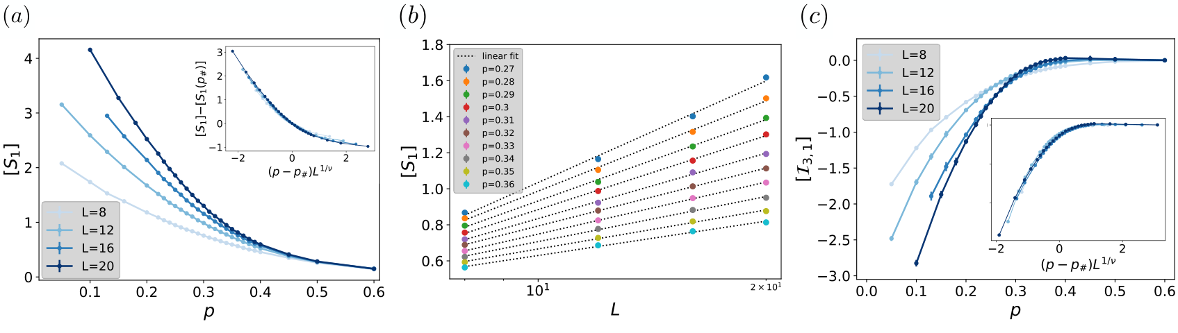
In the statistical model, the total entanglement entropy of the subsystem $A$, $S^{T}_{n}$, depends on the minimal cut which undergoes a percolation transition at $p_{c}=\frac{1}{2}$; for $p<p_{c}$, the length of the minimal cut scales with $L_{A}$ while for $p>p_{c}$ the measurement locations percolate and $\ell_{\rm DW}$ becomes ${\cal O}(1)$. Clearly the total entanglement entropy follows the area law for $p>p_{c}$, and is extensive (and dominated by the qudit contribution) for $p<p_{c}$. As discussed below (20), $S^{T}_{n}$ is given by the sum of two contributions from the qudit and qubit sectors, respectively. In what follows, we will focus on the qubit contribution $S_{n}=S^{T}_{n}-S^{d}_{n}$, and argue that this quantity undergoes an entanglement transition from volume law to area law for $p=p_{\#}$. We will show that this entanglement transition from the qubit sector coincides with a charge-sharpening transition, which can also be diagnosed in a scalable way using a local ancilla probe, as in Sec. III.

Finally, we briefly turn to the dynamics of the Rényi entropies $S_{n}(t)$ using the statistical model. As before, $S_{n}$ is the contribution of the U(1) qubits to the entanglement entropy: the total entropy $S_{n}^{T}$ always grows linearly for $p<p_{c}=1/2$ due to the qudit sector. The results below should be interpreted as sub-leading corrections to the growth of the total entanglement entropy arising due to the slow dynamics of the U(1) qubits.

In the absence of measurements, the statistical mechanics model predicts that all Rényi entropies scale diffusively $S_{n>1}\sim\sqrt{t}$, whereas $S_{n=1}\sim t$, in agreement with earlier results Rakovszky et al. 2019; Huang 2020b; Zhou and Ludwig 2020 (see Appendix C.1). As argued in Sec. II, in the presence of measurements, the “dead regions” responsible for this unusual behavior survive only until a time $t\sim p^{-2/3}$ in typical trajectories. At long times, the overlap of the wavefunction with dead regions is zero, and we expect the trajectory-averaged Rényi entropies $[S_{n}]$ to grow linearly in time for all $p>0$.

References

- Amico et al. (2008) Luigi Amico, Rosario Fazio, Andreas Osterloh, and Vlatko Vedral, “Entanglement in many-body systems,” Reviews of Modern Physics 80, 517–576 (2008), arXiv:0703044 [quant-ph] .
- Horodecki et al. (2009) Ryszard Horodecki, Paweł Horodecki, Michał Horodecki, and Karol Horodecki, “Quantum entanglement,” Reviews of Modern Physics 81, 865–942 (2009), arXiv:0702225 [quant-ph] .
- Eisert et al. (2010) J. Eisert, M. Cramer, and M. B. Plenio, “Colloquium: Area laws for the entanglement entropy,” Reviews of Modern Physics 82, 277–306 (2010).
- Calabrese and Cardy (2009) Pasquale Calabrese and John Cardy, “Entanglement entropy and conformal field theory,” Journal of Physics A: Mathematical and Theoretical 42, 504005 (2009), arXiv:0905.4013 .
- Laflorencie (2016) Nicolas Laflorencie, “Quantum entanglement in condensed matter systems,” Physics Reports 646, 1–59 (2016), arXiv:1512.03388 .
- Preskill (2018) John Preskill, “Quantum {C}omputing in the {NISQ} era and beyond,” Quantum 2, 79 (2018).
- Nahum et al. (2017) Adam Nahum, Jonathan Ruhman, Sagar Vijay, and Jeongwan Haah, “Quantum entanglement growth under random unitary dynamics,” Physical Review X 7, 31016 (2017), arXiv:1608.06950 .
- Nahum et al. (2018) Adam Nahum, Sagar Vijay, and Jeongwan Haah, “Operator Spreading in Random Unitary Circuits,” Physical Review X 8, 21014 (2018), arXiv:1705.08975 .
- Von Keyserlingk et al. (2018) C. W. Von Keyserlingk, Tibor Rakovszky, Frank Pollmann, and S. L. Sondhi, “Operator Hydrodynamics, OTOCs, and Entanglement Growth in Systems without Conservation Laws,” Physical Review X 8, 021013 (2018), arXiv:1705.08910 .
- Zhou and Nahum (2019) Tianci Zhou and Adam Nahum, “Emergent statistical mechanics of entanglement in random unitary circuits,” Physical Review B 99, 174205 (2019), arXiv:1804.09737 .
- Rakovszky et al. (2018) Tibor Rakovszky, Frank Pollmann, and C. W. Von Keyserlingk, “Diffusive Hydrodynamics of Out-of-Time-Ordered Correlators with Charge Conservation,” Physical Review X 8, 031058 (2018), arXiv:1710.09827 .
- Khemani et al. (2018) Vedika Khemani, Ashvin Vishwanath, and David A. Huse, “Operator Spreading and the Emergence of Dissipative Hydrodynamics under Unitary Evolution with Conservation Laws,” Physical Review X 8, 031057 (2018), arXiv:1710.09835 .
- Li et al. (2018) Yaodong Li, Xiao Chen, and Matthew P.A. Fisher, “Quantum Zeno effect and the many-body entanglement transition,” Physical Review B 98, 205136 (2018), arXiv:1808.06134 .
- Skinner et al. (2019) Brian Skinner, Jonathan Ruhman, and Adam Nahum, “Measurement-Induced Phase Transitions in the Dynamics of Entanglement,” Physical Review X 9, 031009 (2019), arXiv:1808.05953 .
- Choi et al. (2020) Soonwon Choi, Yimu Bao, Xiao Liang Qi, and Ehud Altman, “Quantum Error Correction in Scrambling Dynamics and Measurement-Induced Phase Transition,” Physical Review Letters 125, 030505 (2020), arXiv:1903.05124 .
- Gullans and Huse (2020a) Michael J. Gullans and David A. Huse, “Dynamical Purification Phase Transition Induced by Quantum Measurements,” Physical Review X 10, 41020 (2020a), arXiv:1905.05195 .
- Li and Fisher (2021) Yaodong Li and Matthew P.A. Fisher, “Statistical mechanics of quantum error correcting codes,” Physical Review B 103, 104306 (2021), arXiv:2007.03822 .
- Fan et al. (2021) Ruihua Fan, Sagar Vijay, Ashvin Vishwanath, and Yi Zhuang You, “Self-organized error correction in random unitary circuits with measurement,” Physical Review B 103, 174309 (2021), arXiv:2002.12385 .
- Bao et al. (2020) Yimu Bao, Soonwon Choi, and Ehud Altman, “Theory of the phase transition in random unitary circuits with measurements,” Physical Review B 101, 104301 (2020), arXiv:1908.04305 .
- Jian et al. (2020a) Chao Ming Jian, Yi Zhuang You, Romain Vasseur, and Andreas W.W. Ludwig, “Measurement-induced criticality in random quantum circuits,” Physical Review B 101, 104302 (2020a), arXiv:1908.08051 .
- Li et al. (2021) Yaodong Li, Xiao Chen, Andreas W.W. Ludwig, and Matthew P.A. Fisher, “Conformal invariance and quantum nonlocality in critical hybrid circuits,” Physical Review B 104, 104305 (2021), arXiv:2003.12721 .
- Zabalo et al. (2022) A. Zabalo, M. J. Gullans, J. H. Wilson, R. Vasseur, A. W.W. Ludwig, S. Gopalakrishnan, David A. Huse, and J. H. Pixley, “Operator Scaling Dimensions and Multifractality at Measurement-Induced Transitions,” Physical Review Letters 128, 050602 (2022), arXiv:2107.03393 .
- Li et al. (2019) Yaodong Li, Xiao Chen, and Matthew P.A. Fisher, “Measurement-driven entanglement transition in hybrid quantum circuits,” Physical Review B 100, 134306 (2019), arXiv:1901.08092 .
- Chan et al. (2019) Amos Chan, Rahul M. Nandkishore, Michael Pretko, and Graeme Smith, “Unitary-projective entanglement dynamics,” Physical Review B 99, 224307 (2019), arXiv:1808.05949 .
- Cao et al. (2019) Xiangyu Cao, Antoine Tilloy, and Andrea de Luca, “Entanglement in a free fermion chain under continuous monitoring,” SciPost Physics 7, 24 (2019), arXiv:1804.04638 .
- Szyniszewski et al. (2019) M. Szyniszewski, A. Romito, and H. Schomerus, “Entanglement transition from variable-strength weak measurements,” Physical Review B 100, 064204 (2019), arXiv:1903.05452 .
- Gullans and Huse (2020b) Michael J. Gullans and David A. Huse, “Scalable Probes of Measurement-Induced Criticality,” Physical Review Letters 125, 070606 (2020b), arXiv:1910.00020 .
- Zabalo et al. (2020) Aidan Zabalo, Michael J. Gullans, Justin H. Wilson, Sarang Gopalakrishnan, David A. Huse, and J. H. Pixley, “Critical properties of the measurement-induced transition in random quantum circuits,” Physical Review B 101, 060301 (2020), arXiv:1911.00008 .
- Nahum and Skinner (2020) Adam Nahum and Brian Skinner, “Entanglement and dynamics of diffusion-annihilation processes with Majorana defects,” Physical Review Research 2, 23288 (2020), arXiv:1911.11169 .
- Ippoliti et al. (2021) Matteo Ippoliti, Michael J. Gullans, Sarang Gopalakrishnan, David A. Huse, and Vedika Khemani, “Entanglement Phase Transitions in Measurement-Only Dynamics,” Physical Review X 11, 011030 (2021), arXiv:2004.09560 .
- Lavasani et al. (2021) Ali Lavasani, Yahya Alavirad, and Maissam Barkeshli, “Measurement-induced topological entanglement transitions in symmetric random quantum circuits,” Nature Physics 17, 342–347 (2021), arXiv:2004.07243 .
- Sang and Hsieh (2021) Shengqi Sang and Timothy H. Hsieh, “Measurement-protected quantum phases,” Physical Review Research 3, 023200 (2021), arXiv:2004.09509 .
- Tang and Zhu (2020) Qicheng Tang and W. Zhu, “Measurement-induced phase transition: A case study in the nonintegrable model by density-matrix renormalization group calculations,” Physical Review Research 2, 13022 (2020), arXiv:1908.11253 .
- Lopez-Piqueres et al. (2020) Javier Lopez-Piqueres, Brayden Ware, and Romain Vasseur, “Mean-field entanglement transitions in random tree tensor networks,” Physical Review B 102, 64202 (2020), arXiv:2003.01138 .
- Nahum et al. (2021) Adam Nahum, Sthitadhi Roy, Brian Skinner, and Jonathan Ruhman, “Measurement and Entanglement Phase Transitions in All-To-All Quantum Circuits, on Quantum Trees, and in Landau-Ginsburg Theory,” PRX Quantum 2, 10352 (2021), arXiv:2009.11311 .
- Turkeshi et al. (2020) Xhek Turkeshi, Rosario Fazio, and Marcello Dalmonte, “Measurement-induced criticality in (2+1) -dimensional hybrid quantum circuits,” Physical Review B 102, 014315 (2020), arXiv:2007.02970 .
- Fuji and Ashida (2020) Yohei Fuji and Yuto Ashida, “Measurement-induced quantum criticality under continuous monitoring,” Physical Review B 102, 054302 (2020), arXiv:2004.11957 .
- Lunt et al. (2021) Oliver Lunt, Marcin Szyniszewski, and Arijeet Pal, “Measurement-induced criticality and entanglement clusters: A study of one-dimensional and two-dimensional Clifford circuits,” Physical Review B 104, 155111 (2021), arXiv:2012.03857 .
- Lunt and Pal (2020) Oliver Lunt and Arijeet Pal, “Measurement-induced entanglement transitions in many-body localized systems,” Physical Review Research 2, 043072 (2020), arXiv:2005.13603 .
- Vijay (2020) Sagar Vijay, “Measurement-Driven Phase Transition within a Volume-Law Entangled Phase,” arXiv e-prints , arXiv:2005.03052 (2020), arXiv:2005.03052 .
- Turkeshi et al. (2021) Xhek Turkeshi, Alberto Biella, Rosario Fazio, Marcello Dalmonte, and Marco Schiró, “Measurement-induced entanglement transitions in the quantum Ising chain: From infinite to zero clicks,” Physical Review B 103, 224210 (2021), arXiv:2103.09138 .
- Ippoliti and Khemani (2021) Matteo Ippoliti and Vedika Khemani, “Postselection-Free Entanglement Dynamics via Spacetime Duality,” Physical Review Letters 126, 060501 (2021), arXiv:2010.15840 .
- Lu and Grover (2021) Tsung Cheng Lu and Tarun Grover, “Spacetime duality between localization transitions and measurement-induced transitions,” PRX Quantum 2, 1–16 (2021), arXiv:2103.06356 .
- Jian et al. (2020b) Chao-Ming Jian, Bela Bauer, Anna Keselman, and Andreas W. W. Ludwig, “Criticality and entanglement in non-unitary quantum circuits and tensor networks of non-interacting fermions,” (2020b), arXiv:2012.04666 .
- Gopalakrishnan and Gullans (2021) Sarang Gopalakrishnan and Michael J. Gullans, “Entanglement and Purification Transitions in Non-Hermitian Quantum Mechanics,” Physical Review Letters 126, 170503 (2021), arXiv:2012.01435 .
- Turkeshi (2021) Xhek Turkeshi, “Measurement-induced criticality as a data-structure transition,” arXiv e-prints , arXiv:2101.06245 (2021), arXiv:2101.06245 .
- Bao et al. (2021) Yimu Bao, Soonwon Choi, and Ehud Altman, “Symmetry enriched phases of quantum circuits,” Annals of Physics 435, 168618 (2021), arXiv:2102.09164 .
- Block et al. (2022) Maxwell Block, Yimu Bao, Soonwon Choi, Ehud Altman, and Norman Y. Yao, “Measurement-Induced Transition in Long-Range Interacting Quantum Circuits,” Physical Review Letters 128, 010604 (2022), arXiv:2104.13372 .
- Bentsen et al. (2021) Gregory S. Bentsen, Subhayan Sahu, and Brian Swingle, “Measurement-induced purification in large- N hybrid Brownian circuits,” Physical Review B 104, 094304 (2021), arXiv:2104.07688 .
- Noel et al. (2022) Crystal Noel, Pradeep Niroula, Daiwei Zhu, Andrew Risinger, Laird Egan, Debopriyo Biswas, Marko Cetina, Alexey V. Gorshkov, Michael J. Gullans, David A. Huse, and Christopher Monroe, “Measurement-induced quantum phases realized in a trapped-ion quantum computer,” Nature Physics , 760–764 (2022), arXiv:2106.05881 [quant-ph] .
- Friedman et al. (2019) Aaron J. Friedman, Amos Chan, Andrea De Luca, and J. T. Chalker, “Spectral Statistics and Many-Body Quantum Chaos with Conserved Charge,” Physical Review Letters 123, 210603 (2019), arXiv:1906.07736 .
- Rakovszky et al. (2019) Tibor Rakovszky, Frank Pollmann, and C. W. Von Keyserlingk, “Sub-ballistic Growth of Rényi Entropies due to Diffusion,” Physical Review Letters 122, 250602 (2019), arXiv:1901.10502 .
- Huang (2020a) Yichen Huang, “Dynamics of Renyi entanglement entropy in local quantum circuits with charge conservation,” IOPSciNotes 1, 035205 (2020a), arXiv:1902.00977 .
- Zhou and Ludwig (2020) Tianci Zhou and Andreas W.W. Ludwig, “Diffusive scaling of Rényi entanglement entropy,” Physical Review Research 2, 33020 (2020), arXiv:1911.12384 .
- Rakovszky et al. (2020) Tibor Rakovszky, Frank Pollmann, and C W von Keyserlingk, “Comment on ”Entanglement growth in diffusive systems”,” (2020), arXiv:2010.07969 .
- Žnidarič (2020) Marko Žnidarič, “Entanglement growth in diffusive systems,” Communications Physics 3, 1–9 (2020), arXiv:1912.03645 .
- Barratt et al. (2021) Fergus Barratt, Utkarsh Agrawal, Sarang Gopalakrishnan, David A. Huse, Romain Vasseur, and Andrew C. Potter, “Field theory of charge sharpening in symmetric monitored quantum circuits,” arXiv e-prints , arXiv:2111.09336 (2021), arXiv:2111.09336 .
- (58) Since the unitaries acting on the qudits are random, the randomizing measurement basis is superfluous.
- Blais et al. (2021) Alexandre Blais, Arne L. Grimsmo, S. M. Girvin, and Andreas Wallraff, “Circuit quantum electrodynamics,” Reviews of Modern Physics 93, 25005 (2021), arXiv:2005.12667 .
- (60) The ensemble-averaged resulting from maximally-random, local, open-systems dynamics is indistinguishable from an infinite temperature state over distances .
- (61) This can seen by the central limit theorem as follows: assuming each measurement outcome to be independent, the statistical error in the outcomes of the measurement of charge density goes as . To distinguish the states with global charge and , we require this error to become smaller than . This gives .
- Huang (2020b) Yichen Huang, “Dynamics of Rényi entanglement entropy in diffusive qudit systems,” IOP SciNotes 1, 035205 (2020b), arXiv:2008.00944 .
- (63) Though other quantities such as are dominated by rare dead-region contributions and do exhibit growth due to rare dilute measurement locations. The parametrically strong discrepancy between the average purity and the average Rényi entropies is also seen numerically in our statistical model approach (Sec. V).
- (64) To obtain a uniform distribution over we must pick and uniformly and compute .
- (65) In the absence of a conservation law, it has been shown that the probes we have used for the entanglement transition ( and ) have weak finite size drifts in Clifford circuits Zabalo et al. 2020 by examining small and large system sizes.
- Hayden et al. (2016) Patrick Hayden, Sepehr Nezami, Xiao Liang Qi, Nathaniel Thomas, Michael Walter, and Zhao Yang, “Holographic duality from random tensor networks,” Journal of High Energy Physics 2016, 9 (2016), arXiv:1601.01694 .
- Vasseur et al. (2019) Romain Vasseur, Andrew C. Potter, Yi Zhuang You, and Andreas W.W. Ludwig, “Entanglement transitions from holographic random tensor networks,” Physical Review B 100, 134203 (2019), arXiv:1807.07082 .
- (68) DWs are restricted by unitarity to only make certain “turns” (See Zhou and Nahum 2019 for details). E.g, for , this leads to a unique DW where the DW follows a “light cone”. For one can still have many degenerate paths Li and Fisher 2021.
- (69) Any difference in the vertex elements will lead to the creation of DW which are suppressed as and whose contribution goes to zero as .
- (70) Note that the DW permutation element has cycles and each cycle can follow an independent path (to the leading order) Zhou and Nahum 2019. However, this subtlety will not change the final result about the minimal cut, but only leads to fluctuations contributing sub-leading logarithmic corrections (for ).
- (71) Note that this description of the differs from that of Ref. Jian et al. 2020a. There the measurement locations were averaged over directly in the partition function, in an annealed way, while we chose here to keep the measurement locations as quenched disorder. Our approach predicts a minimal cut picture consistent with Ref. Skinner et al. 2019. We leave a discussion of the validity of the replica trick in this limit to future work.
- Schollwöck (2011) Ulrich Schollwöck, “The density-matrix renormalization group in the age of matrix product states,” Annals of Physics 326, 96–192 (2011), arXiv:1008.3477 .
- (73) Frozen in the sense that there is not much quantum superposition of different charge configurations.
- Weinstein et al. (2022) Zack Weinstein, Yimu Bao, and Ehud Altman, “Measurement-induced power law negativity in an open monitored quantum circuit,” (2022).
- Fisher (2004) Matthew Fisher, “Duality in low dimensional quantum field theories,” in Strong interactions in low dimensions (Springer, 2004) pp. 419–438.
- Potter and Vasseur (2016) Andrew C. Potter and Romain Vasseur, “Symmetry constraints on many-body localization,” Physical Review B 94, 224206 (2016), arXiv:1605.03601 .
- Chen et al. (2013) Xie Chen, Zheng Cheng Gu, Zheng Xin Liu, and Xiao Gang Wen, “Symmetry protected topological orders and the group cohomology of their symmetry group,” Physical Review B - Condensed Matter and Materials Physics 87, 155114 (2013), arXiv:1106.4772 .
- Chen et al. (2012) Xie Chen, Zheng Cheng Gu, Zheng Xin Liu, and Xiao Gang Wen, “Symmetry-protected topological orders in interacting bosonic systems,” Science 338, 1604–1606 (2012), arXiv:1301.0861 .
- Chen et al. (2014) Xie Chen, Yuan Ming Lu, and Ashvin Vishwanath, “Symmetry-protected topological phases from decorated domain walls,” Nature Communications 5, 3507 (2014), arXiv:1303.4301 .
- Deng and Blöte (2003) Youjin Deng and Henk W.J. Blöte, “Simultaneous analysis of several models in the three-dimensional Ising universality class,” Physical Review E - Statistical Physics, Plasmas, Fluids, and Related Interdisciplinary Topics 68, 9 (2003).