跳到论文正文
W Papers独立论文阅读器 arXiv:2107.09963 论文正文 计算阅读时间 · 0%
引用这篇论文根据当前论文元数据生成,正式投稿前建议核对。


License: CC BY 4.0
arXiv:2107.09963v1 [math.OC] 21 Jul 2021

Automated computation of topological derivatives with application to nonlinear elasticity and reaction-diffusion problems

Peter Gangl P. GanglTU Graz, Steyrergasse 30/III, 8010 Graz, Austria Email address: gangl(at)math.tugraz.at and Kevin Sturm K. SturmTU Wien, Wiedner Hauptstr. 8-10, 1040 Vienna, Austria Email address: kevin.sturm(at)tuwien.ac.at
Date: August 11, 2026
Abstract.

  
Purpose While topological derivatives have proven useful in applications of topology optimisation and inverse problems, their mathematically rigorous derivation remains an ongoing research topic, in particular in the context of nonlinear partial differential equation (PDE) constraints.
Design/methodology/approach We present a systematic yet formal approach for the computation of topological derivatives of a large class of PDE-constrained topology optimization problems with respect to arbitrary inclusion shapes. Scalar and vector-valued as well as linear and nonlinear elliptic PDE constraints are considered in two and three space dimensions including a nonlinear elasticity model and nonlinear reaction-diffusion problems. The systematic procedure follows a Lagrangian approach for computing topological derivatives.
Findings For problems where the exact formula is known, the numerically computed values show good coincidence. Moreover, by inserting the computed values into the topological asymptotic expansion, we verify that the obtained values satisfy the expected behaviour also for other, previously unknown problems, indicating the correctness of the procedure.
Originality/value We present a systematic approach for the computation of topological derivatives that is applicable to a large class of problems. Most notably, our approach covers the topological derivative for a nonlinear elasticity problem, which has not been reported in the literature.

Key words and phrases: 
topological derivative, automated differentiation, nonlinear elasticity, nonlinear diffusion-convection-reaction equation

1. Introduction

The topological derivative concept was first used for finding optimal locations of holes in mechanical structures in [11] and was later introduced in a mathematically concise way in the publications [22] and [17]. Given a shape function 𝒥\mathcal{J} that maps a shape Ω\Omega to a real number 𝒥⁡(Ω)\mathcal{J}(\Omega), the topological derivative at a spatial point z∈Ωz\in\Omega measures the sensitivity of 𝒥\mathcal{J} with respect to a small topological perturbation of the shape Ω\Omega. Denoting the perturbed shape by Ωε\Omega_{\varepsilon}, e.g., Ωε:=Ω∖ωε\Omega_{\varepsilon}:=\Omega\setminus\omega_{\varepsilon} with ωε=Bε​(z)\omega_{\varepsilon}=B_{\varepsilon}(z), the topological derivative is defined as

d​𝒥​(Ω)​(z):=lim ε↘0​𝒥⁡(Ωε)−𝒥⁡(Ω)|ωε|,\displaystyle d\mathcal{J}(\Omega)(z):=\underset{{\varepsilon}\searrow 0}{\mbox{lim }}\frac{\mathcal{J}(\Omega_{\varepsilon})-\mathcal{J}(\Omega)}{|\omega_{\varepsilon}|}, (1.1)

thus satisfying a topologically asymptotic expansion of the form

𝒥⁡(Ωε)=𝒥⁡(Ω)+|ωε|​d​𝒥​(Ω)​(z)+o⁡(ε)as ​ε↘0.\displaystyle\mathcal{J}(\Omega_{\varepsilon})=\mathcal{J}(\Omega)+|\omega_{\varepsilon}|d\mathcal{J}(\Omega)(z)+o({\varepsilon})\quad\mbox{as }{\varepsilon}\searrow 0. (1.2)

Since its introduction, the topological derivative concept has found application mostly in the context of topology optimization for engineering applications by level set approaches [4, 1, 9], but has also been utilized in medical applications such as electrical impedance tomography (EIT) [19] or mathematical image processing [18].

Most practically relevant engineering applications involve a partial differential equation (PDE) constraint and thus are of the type

inf Ω​J​(Ω,u)subject to ​e​(Ω,u)=0\displaystyle\underset{\Omega}{\mbox{inf }}J(\Omega,u)\qquad\mbox{subject to }\;e(\Omega;u)=0 (1.3)

with a PDE operator e⁡(Ω,⋅)e(\Omega;\cdot). In many cases (in particular when the principal part of the PDE operator is subject to a topological perturbation), the derivation of topological derivatives involves an asymptotic analysis of the state variable of the form

uε​(z+ε​x)=u0​(z+ε​x)+ε​K​(x)+o⁡(ε) as ​ε↘0,\displaystyle u_{\varepsilon}(z+{\varepsilon}x)=u_{0}(z+{\varepsilon}x)+{\varepsilon}K(x)+o({\varepsilon})\quad\mbox{ as }{\varepsilon}\searrow 0, (1.4)

where uεu_{\varepsilon} is defined by the perturbed PDE operator, e⁡(Ωε,uε)=0e(\Omega_{\varepsilon},u_{\varepsilon})=0, and KK is a corrector function defined as the solution to a transmission problem on the unbounded domain 𝐑d{\mathbf{R}}^{d}. Often, also a similar asymptotic analysis of an adjoint variable is needed. There exist different approaches for the derivation of topological derivatives for PDE-constrained optimization problems of the type (1.3). We mention the approaches by Novotny and Sokolowski [20], the approach by Amstutz [3] as well as the averaged adjoint approach [23]. Finally, we mention the approach that was introduced by Delfour in [10] and applied to quasilinear problems in [12, 14], which does not involve an asymptotic analysis of an adjoint variable.

For many problems involving linear or semilinear PDE constraints, topological derivatives are rather well-understood. In the cases where the shape of the inclusion ω\omega is a disk or ellipse in 2D or a ball or ellipsoid in 3D, the corrector function KK can be determined analytically and the topological derivative can be obtained in a closed form involving so-called polarisation tensors [2]. When ω\omega has a more general shape as well as in the case of quasilinear PDE constraints, explicit formulas have not been reported in the literature. Topological derivatives in the context of quasilinear PDE constraints were first treated theoretically in [5], and later also in [12]. The numerical computation for a quasilinear problem was first discussed in [6] in the context of two-dimensional nonlinear magnetostatics, and later in the context of three-dimensional nonlinear magnetostatics in an H⁡(c​u​r​l)H(curl) setting in [14].

In this paper, we make the assumption that an expansion of the form (1.4) holds and apply the systematic approach of M.C. Delfour [10], see also [12], to a large class of problems involving linear and nonlinear elliptic PDEs as constraints. The suggested procedure covers scalar and vector-valued problems in two and three space dimensions. In particular, we will also treat the problem of nonlinear elasticity in two space dimensions using a St. Venant-Kirchhoff material which, to the best of the authors’ knowledge, has not been reported on in the literature so far.

We stress that our generic automated approach is formal since a rigorous derivation would require a detailed asymptotic analysis of the variation of the state (1.4). Usually, this entails to show a sufficiently fast decay of the corrector KK as |x|→∞|x|\rightarrow\infty. While the computation is formal, we show numerically that, for the considered problems, the computed values satisfy a topologically asymptotic expansion of the form (1.2).

2. Lagrangian approach for computing topological derivatives

In this section, we present the general approach for computing topological derivatives of a class of model problems based on the Lagrangian approach introduced in [10]. The considered problems include linear and nonlinear, scalar and vector-valued elliptic PDE constraints in two or three space dimensions.

2.1. Class of considered problems

We consider a PDE-constrained shape optimization problem in dd space dimensions where the solution to the PDE is 𝐑m{\mathbf{R}}^{m}-valued. This covers the case of scalar quantities, m=1m=1 or vector-valued problems such as elasticity, m=dm=d. For a function φ:𝐑d→𝐑m\varphi:{\mathbf{R}}^{d}\rightarrow{\mathbf{R}}^{m}, we denote by 𝒟​φ∈𝐑m×d\mathcal{D}\varphi\in{\mathbf{R}}^{m\times d} its Jacobian, (𝒟​φ)i,k=∂φi∂xk(\mathcal{D}\varphi)_{i,k}=\frac{\partial\varphi_{i}}{\partial x_{k}} for i∈{1,…​m},k∈{1,…​d}i\in\{1,\dots m\},k\in\{1,\dots d\}. We recall the Euclidean vector product a⋅b=∑i=1mai​bia\cdot b=\sum_{i=1}^{m}a_{i}b_{i} for a,b∈𝐑ma,b\in{\mathbf{R}}^{m} and will also use this notation for m=1m=1, noting that the vector product is just a simple product then. Moreover, we denote by A:B=∑i=1m∑k=1dAi,k​Bi,kA:B=\sum_{i=1}^{m}\sum_{k=1}^{d}A_{i,k}B_{i,k} the Frobenius inner product of two matrices A,B∈𝐑m×dA,B\in{\mathbf{R}}^{m\times d} and again note that the Frobenius inner product reduces to the Euclidean inner product of two vectors when m=1m=1.

We consider a computational domain 𝖣\mathsf{D} which is subdivided into two open disjoint subdomains, 𝖣=Ωin∪Ωout\mathsf{D}=\Omega^{\text{in}}\cup\Omega^{\text{out}}. We introduce the abbreviation Ω:=Ωin\Omega:=\Omega^{\text{in}}, such that Ωout=𝖣∖Ω¯\Omega^{\text{out}}=\mathsf{D}\setminus\overline{\Omega}. Moreover, we consider four operators

A1in,A1out:\displaystyle A_{1}^{\text{in}},A_{1}^{\text{out}}: 𝖣×𝐑m×𝐑m×d→𝐑m\displaystyle\,\mathsf{D}\times{\mathbf{R}}^{m}\times{\mathbf{R}}^{m\times d}\rightarrow{\mathbf{R}}^{m}
A2in,A2out:\displaystyle A_{2}^{\text{in}},A_{2}^{\text{out}}: 𝖣×𝐑m×𝐑m×d→𝐑m×d\displaystyle\,\mathsf{D}\times{\mathbf{R}}^{m}\times{\mathbf{R}}^{m\times d}\rightarrow{\mathbf{R}}^{m\times d}

to define the two piecewise defined operators A1Ω:𝖣×𝐑m×𝐑m×d→𝐑mA_{1}^{\Omega}:\mathsf{D}\times{\mathbf{R}}^{m}\times{\mathbf{R}}^{m\times d}\rightarrow{\mathbf{R}}^{m}, A2Ω:𝖣×𝐑m×𝐑m×d→𝐑m×dA_{2}^{\Omega}:\mathsf{D}\times{\mathbf{R}}^{m}\times{\mathbf{R}}^{m\times d}\rightarrow{\mathbf{R}}^{m\times d},

A1Ω​(x,y1,y2):=χΩ​(x)​A1in​(x,y1,y2)+χ𝖣∖Ω​(x)​A1out​(x,y1,y2),\displaystyle A_{1}^{\Omega}(x,y_{1},y_{2}):=\chi_{\Omega}(x)A_{1}^{\text{in}}(x,y_{1},y_{2})+\chi_{\mathsf{D}\setminus\Omega}(x)A_{1}^{\text{out}}(x,y_{1},y_{2}), (2.1)
A2Ω​(x,y1,y2):=χΩ​(x)​A2in​(x,y1,y2)+χ𝖣∖Ω​(x)​A2out​(x,y1,y2),\displaystyle A_{2}^{\Omega}(x,y_{1},y_{2}):=\chi_{\Omega}(x)A_{2}^{\text{in}}(x,y_{1},y_{2})+\chi_{\mathsf{D}\setminus\Omega}(x)A_{2}^{\text{out}}(x,y_{1},y_{2}), (2.2)

which will represent the left hand side of an abstract PDE constraint. The right hand side will comprise F1Ω:𝖣→𝐑mF_{1}^{\Omega}:\mathsf{D}\rightarrow{\mathbf{R}}^{m}, F2Ω:𝖣→𝐑m×dF_{2}^{\Omega}:\mathsf{D}\rightarrow{\mathbf{R}}^{m\times d} with

FiΩ​(x):=χΩ​(x)​Fiin​(x)+χ𝖣∖Ω​(x)​Fiout​(x),\displaystyle F_{i}^{\Omega}(x):=\chi_{\Omega}(x)F_{i}^{\text{in}}(x)+\chi_{\mathsf{D}\setminus\Omega}(x)F_{i}^{\text{out}}(x), (2.3)

for i=1,2i=1,2 with functions F1in,F1out:𝖣→𝐑mF_{1}^{\text{in}},F_{1}^{\text{out}}:\mathsf{D}\rightarrow{\mathbf{R}}^{m} and F2in,F2out:𝖣→𝐑m×dF_{2}^{\text{in}},F_{2}^{\text{out}}:\mathsf{D}\rightarrow{\mathbf{R}}^{m\times d}. Finally, we assume that the boundary ∂𝖣\partial\mathsf{D} of 𝖣\mathsf{D} is subdivided into two subsets ΓD,ΓN\Gamma_{D},\Gamma_{N} and consider a function gN:ΓN→𝐑mg_{N}:\Gamma_{N}\rightarrow{\mathbf{R}}^{m} to represent inhomogeneous Neumann boundary conditions. For sake of more compact presentation, we only consider homogeneous Dirichlet conditions on the Dirichlet boundary ΓD\Gamma_{D} and remark that an extension to inhomogenous conditions can be obtained by minor modifications. For a given admissible subdomain Ω⊂𝖣\Omega\subset\mathsf{D}, we consider the PDE constraint to find u∈𝐄⁡(𝖣)u\in{\mathbf{E}}(\mathsf{D}) such that

∫𝖣A1Ω​(x,u,𝒟​u)⋅ψ+A2Ω​(x,u,𝒟​u):𝒟​ψ​d​x=∫𝖣F1Ω​(x)⋅ψ+F2Ω​(x):𝒟​ψ​d​x+∫ΓNgN⋅ψ​d​S\displaystyle\int_{\mathsf{D}}A_{1}^{\Omega}(x,u,\mathcal{D}u)\cdot\psi+A_{2}^{\Omega}(x,u,\mathcal{D}u):\mathcal{D}\psi\;\mbox{d}x=\int_{\mathsf{D}}F_{1}^{\Omega}(x)\cdot\psi+F_{2}^{\Omega}(x):\mathcal{D}\psi\;\mbox{d}x+\int_{\Gamma_{N}}g_{N}\cdot\psi\;\mbox{d}S (2.4)

for all ψ∈𝐄⁡(𝖣)\psi\in{\mathbf{E}}(\mathsf{D}), where 𝐄⁡(𝖣){\mathbf{E}}(\mathsf{D}) is the function space on which the PDE is posed and which includes the homogeneous Dirichlet conditions on ΓD\Gamma_{D}. Similarly, we consider two functions jin,jout:𝖣×𝐑m×𝐑m×d→𝐑j^{\text{in}},j^{\text{out}}:\mathsf{D}\times{\mathbf{R}}^{m}\times{\mathbf{R}}^{m\times d}\rightarrow{\mathbf{R}} and, for a given admissible set Ω⊂𝖣\Omega\subset\mathsf{D}, define the piecewise defined function jΩ:𝖣×𝐑m×𝐑m×d→𝐑j^{\Omega}:\mathsf{D}\times{\mathbf{R}}^{m}\times{\mathbf{R}}^{m\times d}\rightarrow{\mathbf{R}},

jΩ​(x,y1,y2):=χΩ​(x)​jin​(x,y1,y2)+χ𝖣∖Ω​(x)​jout​(x,y1,y2).\displaystyle j^{\Omega}(x,y_{1},y_{2}):=\chi_{\Omega}(x)j^{\text{in}}(x,y_{1},y_{2})+\chi_{\mathsf{D}\setminus\Omega}(x)j^{\text{out}}(x,y_{1},y_{2}). (2.5)

For φ∈𝐄⁡(𝖣)\varphi\in{\mathbf{E}}(\mathsf{D}), we will consider the cost function

J⁡(Ω,φ,𝒟​φ):=Jvol​(Ω,φ,𝒟​φ)+Jbnd​(φ,𝒟​φ)\displaystyle J(\Omega,\varphi,\mathcal{D}\varphi):=J^{\text{vol}}(\Omega,\varphi,\mathcal{D}\varphi)+J^{\text{bnd}}(\varphi,\mathcal{D}\varphi) (2.6)

with

Jvol​(Ω,φ,𝒟​φ):=∫𝖣jΩ​(x,φ,𝒟​φ)​𝑑x,Jbnd​(φ,𝒟​φ):=∫∂𝖣jb​n​d​(x,φ,𝒟​φ)​𝑑S\displaystyle J^{\text{vol}}(\Omega,\varphi,\mathcal{D}\varphi):=\int_{\mathsf{D}}j^{\Omega}(x,\varphi,\mathcal{D}\varphi)\;dx,\qquad J^{\text{bnd}}(\varphi,\mathcal{D}\varphi):=\int_{\partial\mathsf{D}}j^{bnd}(x,\varphi,\mathcal{D}\varphi)\;dS (2.7)

for a function jb​n​d:∂𝖣×𝐑m×𝐑m×d→𝐑j^{bnd}:\partial\mathsf{D}\times{\mathbf{R}}^{m}\times{\mathbf{R}}^{m\times d}\rightarrow{\mathbf{R}}. Summarizing, we consider the abstract class of PDE-constrained topology optimization problem which can be written as

min Ω∈𝒜​Jvol​(Ω,u,𝒟​u)+Jbnd​(u,𝒟​u)subject to ​u∈𝐄⁡(𝖣)​ solves (2.4)\displaystyle\begin{aligned} &\underset{\Omega\in\mathcal{A}}{\mbox{min }}J^{\text{vol}}(\Omega,u,\mathcal{D}u)+J^{\text{bnd}}(u,\mathcal{D}u)\\ &\mbox{subject to }u\in{\mathbf{E}}(\mathsf{D})\mbox{ solves }\eqref{eq_abstr_pde}\end{aligned} (2.8)

where 𝒜\mathcal{A} denotes the set of admissible subsets of 𝖣\mathsf{D}.

Remark 1.

Although we consider only homogeneous boundary conditions, the formulas for inhomogeneous Dirichlet boundary conditions will not affect the formula of the first topological derivative; see, e.g., [8] where mixed (Dirichlet and Neumann) inhomogeneous boundary conditions are considered.

2.2. Domain perturbation

Let ω⊂𝐑d\omega\subset{\mathbf{R}}^{d} with 0∈ω0\in\omega represent the shape of the considered topological perturbation. For a point z∈𝖣∖∂Ωz\in\mathsf{D}\setminus\partial\Omega and a given small parameter ε{\varepsilon}, we define ωε​(z):=z+ε​ω\omega_{\varepsilon}(z):=z+{\varepsilon}\omega as well as the perturbed domain

Ωε​(z):={Ω∖ω¯ε​(z),z∈Ω,Ω∪ωε​(z),z∈𝖣∖Ω¯.\displaystyle\Omega_{\varepsilon}(z):=\begin{cases}\Omega\setminus\overline{\omega}_{\varepsilon}(z),&z\in\Omega,\\ \Omega\cup\omega_{\varepsilon}(z),&z\in\mathsf{D}\setminus\overline{\Omega}.\end{cases}

From now on, we assume that a fixed point z∈𝖣∖Ω¯z\in\mathsf{D}\setminus\overline{\Omega} is given and set ωε:=ωε​(z)\omega_{\varepsilon}:=\omega_{\varepsilon}(z), Ωε:=Ωε​(z)\Omega_{\varepsilon}:=\Omega_{\varepsilon}(z). Moreover, we use the abbreviation 𝖣ε:=Tε−1​(𝖣)\mathsf{D}_{\varepsilon}:=T_{\varepsilon}^{-1}(\mathsf{D}), where Tε​(x):=z+ε​xT_{\varepsilon}(x):=z+{\varepsilon}x. We also introduce the abbreviating notations A1(ε):=A1ΩεA_{1}^{({\varepsilon})}:=A_{1}^{\Omega_{\varepsilon}}, A2(ε):=A2ΩεA_{2}^{({\varepsilon})}:=A_{2}^{\Omega_{\varepsilon}}, F1(ε):=F1ΩεF_{1}^{({\varepsilon})}:=F_{1}^{\Omega_{\varepsilon}}, F2(ε):=F2ΩεF_{2}^{({\varepsilon})}:=F_{2}^{\Omega_{\varepsilon}}, j(ε):=jΩεj^{({\varepsilon})}:=j^{\Omega_{\varepsilon}} and define the perturbed Lagrangian of the abstract optimization problem (2.8)

G⁡(ε,φ,𝒟​φ,ψ,𝒟​ψ)=\displaystyle G({\varepsilon},\varphi,\mathcal{D}\varphi,\psi,\mathcal{D}\psi)= J⁡(Ωε,φ,𝒟​φ)+⟨A1(ε)​(φ,𝒟​φ),ψ⟩+⟨A2(ε)​(φ,𝒟​φ),𝒟​ψ⟩\displaystyle\,J(\Omega_{\varepsilon},\varphi,\mathcal{D}\varphi)+\langle A_{1}^{({\varepsilon})}(\varphi,\mathcal{D}\varphi),\psi\rangle+\langle A_{2}^{({\varepsilon})}(\varphi,\mathcal{D}\varphi),\mathcal{D}\psi\rangle
−⟨F1(ε),ψ⟩−⟨F2(ε),𝒟​ψ⟩−⟨gN,ψ⟩,\displaystyle-\langle F_{1}^{({\varepsilon})},\psi\rangle-\langle F_{2}^{({\varepsilon})},\mathcal{D}\psi\rangle-\langle g_{N},\psi\rangle,

where ⟨⋅,⋅⟩\langle\cdot,\cdot\rangle denotes the duality product in the corresponding spaces.

2.3. Formal variation of the state variable

The following derivation is motivated by the rigorous results obtained in [12], where a simplified approach to the computation of quasi-linear derivatives is proposed. Here we generalise these results formally to the class of non-linear problems introduced in (2.8). We also refer to [6, 5] for another approach to the computation of topological derivatives for quasi-linear problems.

Let ψ∈𝐄⁡(𝖣)\psi\in{\mathbf{E}}(\mathsf{D}). The perturbed state equation reads: uεu_{\varepsilon} solves

∫𝖣A1(ε)​(x,uε,𝒟​uε)⋅ψ+A2(ε)​(x,uε,𝒟​uε):𝒟​ψ​𝑑x=∫𝖣F1(ε)​(x)⋅ψ+F2(ε)​(x):𝒟​ψ​d​x+∫ΓNgN⋅ψdS.\displaystyle\begin{split}\int_{\mathsf{D}}A_{1}^{({\varepsilon})}(x,u_{\varepsilon},\mathcal{D}u_{\varepsilon})\cdot\psi+A_{2}^{({\varepsilon})}(x,u_{\varepsilon},\mathcal{D}u_{\varepsilon}):\mathcal{D}\psi\;dx=\int_{\mathsf{D}}F_{1}^{({\varepsilon})}(x)\cdot\psi&+F_{2}^{({\varepsilon})}(x):\mathcal{D}\psi\;dx\\ &+\int_{\Gamma_{N}}g_{N}\cdot\psi\;dS.\end{split} (2.9)

Subtracting the state equation (2.9) for ε>0{\varepsilon}>0 from the state equation for ε=0{\varepsilon}=0 leads to

∫𝖣[A1(ε)(x,uε,𝒟uε)−A1(0)(x,u0,𝒟u0)]⋅ψ+[A2(ε)(x,uε,𝒟uε)−A2(0)(x,u0,𝒟u0)]:𝒟ψdx=∫ωε(F1in−F1out)​(x)⋅ψ+(F2in−F2out)​(x):𝒟​ψ​dx.\displaystyle\begin{split}\int_{\mathsf{D}}[A_{1}^{({\varepsilon})}(x,u_{\varepsilon},\mathcal{D}u_{\varepsilon})-&A_{1}^{(0)}(x,u_{0},\mathcal{D}u_{0})]\cdot\psi+[A_{2}^{({\varepsilon})}(x,u_{\varepsilon},\mathcal{D}u_{\varepsilon})-A_{2}^{(0)}(x,u_{0},\mathcal{D}u_{0})]:\mathcal{D}\psi\;dx\\ &=\int_{\omega_{\varepsilon}}(F_{1}^{\text{in}}-F_{1}^{\text{out}})(x)\cdot\psi+(F_{2}^{\text{in}}-F_{2}^{\text{out}})(x):\mathcal{D}\psi\;dx.\end{split}

Using the change of variables Tε​(x)=z+ε​xT_{\varepsilon}(x)=z+{\varepsilon}x, we obtain with the notation 𝖣ε=Tε−1​(𝖣)\mathsf{D}_{\varepsilon}=T_{\varepsilon}^{-1}(\mathsf{D}):

∫𝖣ε\displaystyle\int_{\mathsf{D}_{\varepsilon}} [A1(ε)​(Tε​(x),uε∘Tε,(𝒟​uε)∘Tε)−A1(0)​(Tε​(x),u0∘Tε,(𝒟​u0)∘Tε)]⋅(ψ∘Tε)\displaystyle[A_{1}^{({\varepsilon})}(T_{\varepsilon}(x),u_{\varepsilon}\circ T_{\varepsilon},(\mathcal{D}u_{\varepsilon})\circ T_{\varepsilon})-A_{1}^{(0)}(T_{\varepsilon}(x),u_{0}\circ T_{\varepsilon},(\mathcal{D}u_{0})\circ T_{\varepsilon})]\cdot(\psi\circ T_{\varepsilon})
+\displaystyle+ [A2(ε)​(Tε​(x),uε∘Tε,(𝒟​uε)∘Tε)−A2(0)​(Tε​(x),u0∘Tε,(𝒟​u0)∘Tε)]:(𝒟​ψ)∘Tε​d​x\displaystyle[A_{2}^{({\varepsilon})}(T_{\varepsilon}(x),u_{\varepsilon}\circ T_{\varepsilon},(\mathcal{D}u_{\varepsilon})\circ T_{\varepsilon})-A_{2}^{(0)}(T_{\varepsilon}(x),u_{0}\circ T_{\varepsilon},(\mathcal{D}u_{0})\circ T_{\varepsilon})]:(\mathcal{D}\psi)\circ T_{\varepsilon}\;dx
=∫ω((F1in−F1out)∘Tε)⋅(ψ∘Tε)+((F2in−F2out)∘Tε):((𝒟​ψ)∘Tε)​𝑑x.\displaystyle=\int_{\omega}((F_{1}^{\text{in}}-F_{1}^{\text{out}})\circ T_{\varepsilon})\cdot(\psi\circ T_{\varepsilon})+((F_{2}^{\text{in}}-F_{2}^{\text{out}})\circ T_{\varepsilon}):((\mathcal{D}\psi)\circ T_{\varepsilon})\;dx.

Using (𝒟​φ)∘Tε=1ε​𝒟​(φ∘Tε)(\mathcal{D}\varphi)\circ T_{\varepsilon}=\frac{1}{{\varepsilon}}\mathcal{D}(\varphi\circ T_{\varepsilon}) and the first variation of the state Kε:=(uε−u0)∘TεεK_{\varepsilon}:=\frac{(u_{\varepsilon}-u_{0})\circ T_{\varepsilon}}{{\varepsilon}}, after multiplication with ε{\varepsilon}, we obtain

∫𝖣ε\displaystyle\int_{\mathsf{D}_{\varepsilon}} [A1(ε)(Tε(x),u0∘Tε+εKε,(𝒟u0)∘Tε+𝒟Kε)\displaystyle[A_{1}^{({\varepsilon})}(T_{\varepsilon}(x),u_{0}\circ T_{\varepsilon}+{\varepsilon}K_{\varepsilon},(\mathcal{D}u_{0})\circ T_{\varepsilon}+\mathcal{D}K_{\varepsilon})
−A1(0)(Tε(x),u0∘Tε,(𝒟u0)∘Tε)]⋅(εψ∘Tε)\displaystyle\hskip 113.81102pt-A_{1}^{(0)}(T_{\varepsilon}(x),u_{0}\circ T_{\varepsilon},(\mathcal{D}u_{0})\circ T_{\varepsilon})]\cdot({\varepsilon}\psi\circ T_{\varepsilon})
+\displaystyle+ ∫𝖣ε[A2(ε)(Tε(x),u0∘Tε+εKε,(𝒟u0)∘Tε+𝒟Kε)\displaystyle\int_{\mathsf{D}_{\varepsilon}}[A_{2}^{({\varepsilon})}(T_{\varepsilon}(x),u_{0}\circ T_{\varepsilon}+{\varepsilon}K_{\varepsilon},(\mathcal{D}u_{0})\circ T_{\varepsilon}+\mathcal{D}K_{\varepsilon})
−A2(0)(Tε(x),u0∘Tε,(𝒟u0)∘Tε)]:𝒟(ψ∘Tε)dx\displaystyle\hskip 142.26378pt-A_{2}^{(0)}(T_{\varepsilon}(x),u_{0}\circ T_{\varepsilon},(\mathcal{D}u_{0})\circ T_{\varepsilon})]:\mathcal{D}(\psi\circ T_{\varepsilon})\;dx
=∫ω((F1in−F1out)∘Tε)⋅(ε​ψ∘Tε)+((F2in−F2out)∘Tε):𝒟⁡(ψ∘Tε)​𝑑x.\displaystyle=\int_{\omega}((F_{1}^{\text{in}}-F_{1}^{\text{out}})\circ T_{\varepsilon})\cdot({\varepsilon}\psi\circ T_{\varepsilon})+((F_{2}^{\text{in}}-F_{2}^{\text{out}})\circ T_{\varepsilon}):\mathcal{D}(\psi\circ T_{\varepsilon})\;dx.

Now we make the following assumption:

Assumption 1.
  • (i)

    We assume that u0u_{0} is continuously differentiable at zz.

  • (ii)

    Let Kε:=(uε−u0)∘TεεK_{\varepsilon}:=\frac{(u_{\varepsilon}-u_{0})\circ T_{\varepsilon}}{{\varepsilon}} for ε>0{\varepsilon}>0 be the first variation of the state variable uεu_{\varepsilon}. We assume that ∇Kε→∇K\nabla K_{\varepsilon}\to\nabla K and ε​Kε→0{\varepsilon}K_{\varepsilon}\to 0, where KK solves (2.11).

  • (iii)

    For all ε>0{\varepsilon}>0 we have ψ∈𝐄⁡(𝖣ε)\psi\in{\mathbf{E}}(\mathsf{D}_{\varepsilon}) if and only if ψ∘Tε∈𝐄⁡(𝖣)\psi\circ T_{\varepsilon}\in{\mathbf{E}}(\mathsf{D}).

Rearranging and replacing ψ∘Tε\psi\circ T_{\varepsilon} by ψ\psi (using Assumption 1,item (iii)) yields

∫𝖣ε[A1(ε)​(Tε​(x),u0∘Tε+ε​Kε,(𝒟​u0)∘Tε+𝒟​Kε)−A1(ε)​(Tε​(x),u0∘Tε,(𝒟​u0)∘Tε)]⋅ε​ψ+[A2(ε)​(Tε​(x),u0∘Tε+ε​Kε,(𝒟​u0)∘Tε+𝒟​Kε)−A2(ε)​(Tε​(x),u0∘Tε,(𝒟​u0)∘Tε)]:𝒟​ψ​d​x=∫ω((F1in−F1out)∘Tε)⋅(ε​ψ)+((F2in−F2out)∘Tε):𝒟​ψ​𝑑x−∫ω[A1in−A1out](Tε(x),u0∘Tε,(𝒟u0)∘Tε)⋅εψdx−∫ω[A2in−A2out](Tε(x),u0∘Tε,(𝒟u0)∘Tε):𝒟ψdx\begin{split}\int_{\mathsf{D}_{\varepsilon}}&[A_{1}^{({\varepsilon})}(T_{\varepsilon}(x),u_{0}\circ T_{\varepsilon}+{\varepsilon}K_{\varepsilon},(\mathcal{D}u_{0})\circ T_{\varepsilon}+\mathcal{D}K_{\varepsilon})-A_{1}^{({\varepsilon})}(T_{\varepsilon}(x),u_{0}\circ T_{\varepsilon},(\mathcal{D}u_{0})\circ T_{\varepsilon})]\cdot{\varepsilon}\psi\\ +&[A_{2}^{({\varepsilon})}(T_{\varepsilon}(x),u_{0}\circ T_{\varepsilon}+{\varepsilon}K_{\varepsilon},(\mathcal{D}u_{0})\circ T_{\varepsilon}+\mathcal{D}K_{\varepsilon})-A_{2}^{({\varepsilon})}(T_{\varepsilon}(x),u_{0}\circ T_{\varepsilon},(\mathcal{D}u_{0})\circ T_{\varepsilon})]:\mathcal{D}\psi\;dx\\ =&\int_{\omega}((F_{1}^{\text{in}}-F_{1}^{\text{out}})\circ T_{\varepsilon})\cdot({\varepsilon}\psi)+((F_{2}^{\text{in}}-F_{2}^{\text{out}})\circ T_{\varepsilon}):\mathcal{D}\psi\;dx\\ &-\int_{\omega}[A_{1}^{\text{in}}-A_{1}^{\text{out}}](T_{\varepsilon}(x),u_{0}\circ T_{\varepsilon},(\mathcal{D}u_{0})\circ T_{\varepsilon})\cdot{\varepsilon}\psi\;dx\\ &-\int_{\omega}[A_{2}^{\text{in}}-A_{2}^{\text{out}}](T_{\varepsilon}(x),u_{0}\circ T_{\varepsilon},(\mathcal{D}u_{0})\circ T_{\varepsilon}):\mathcal{D}\psi\;dx\end{split} (2.10)

for all ψ∈𝐄⁡(𝖣ε)\psi\in{\mathbf{E}}(\mathsf{D}_{\varepsilon}). With this we can pass to limit ε→0{\varepsilon}\rightarrow 0 in (2.10) and get

∫𝐑d[A2ω​(z,u0​(z),𝒟​u0​(z)+𝒟​K)−A2ω​(z,u0​(z),𝒟​u0​(z))]:𝒟​ψ​d​x=∫ω(F2in−F2out)​(z):𝒟​ψ​dx−∫ω[A2in−A2out]​(z,u0​(z),𝒟​u0​(z)):𝒟​ψ​dx,\displaystyle\begin{split}\int_{{\mathbf{R}}^{d}}&[A_{2}^{\omega}(z,u_{0}(z),\mathcal{D}u_{0}(z)+\mathcal{D}K)-A_{2}^{\omega}(z,u_{0}(z),\mathcal{D}u_{0}(z))]:\mathcal{D}\psi\;dx\\ &=\int_{\omega}(F_{2}^{\text{in}}-F_{2}^{\text{out}})(z):\mathcal{D}\psi\;dx-\int_{\omega}[A_{2}^{\text{in}}-A_{2}^{\text{out}}](z,u_{0}(z),\mathcal{D}u_{0}(z)):\mathcal{D}\psi\;dx,\end{split} (2.11)

for all ψ∈𝐄⁡(𝐑d):=limε↘0𝐄⁡(𝖣ε)\psi\in{\mathbf{E}}({\mathbf{R}}^{d}):=\lim_{{\varepsilon}\searrow 0}{\mathbf{E}}(\mathsf{D}_{\varepsilon}) , with the definition A2ω​(x,y1,y2)=χω​(x)​A2in​(x,y1,y2)+χ𝐑d∖ω​(x)​A2out​(x,y1,y2)A_{2}^{\omega}(x,y_{1},y_{2})=\chi_{\omega}(x)A_{2}^{\text{in}}(x,y_{1},y_{2})+\chi_{{\mathbf{R}}^{d}\setminus\omega}(x)A_{2}^{\text{out}}(x,y_{1},y_{2}). The limit limε↘0𝐄⁡(𝖣ε)\lim_{{\varepsilon}\searrow 0}{\mathbf{E}}(\mathsf{D}_{\varepsilon}) has to be understood formally and in practice often is a Beppo-Levi space (see the next remark).

Remark 2.

The function space 𝐄⁡(𝐑d){\mathbf{E}}({\mathbf{R}}^{d}) in which (2.11) admits a solution can often be chosen as a Beppo-Levi space as shown in [23], see also [12]. For the numerical approximation in the next section we use precisely that the functions KεK_{\varepsilon} converge to KK and approximate KK by solving an equation on a blown up domain similarly to 𝖣ε\mathsf{D}_{\varepsilon}.

2.4. Lagrangian theorem for first topological derivatives

In this section we discuss a method proposed by M.C. Delfour in [10, Thm.3.3]. The definite advantage is that it uses the unperturbed adjoint equation and only requires the asymptotic analysis of the state equation, but it seems to come with the shortcoming that certain cost functions cannot be treated rigorously; see [12] and also [8].

Let 𝐄⁡(𝖣){\mathbf{E}}(\mathsf{D}) be a Banach space of functions on 𝖣\mathsf{D}. For all parameter ε≥0{\varepsilon}\geq 0 small consider a function uε∈𝐄⁡(𝖣)u_{\varepsilon}\in{\mathbf{E}}(\mathsf{D}) solving the variational problem of the form

aε​[uε]​(φ)=fε​(φ) for all ​φ∈𝐄⁡(𝖣),a_{\varepsilon}[u_{\varepsilon}](\varphi)=f_{\varepsilon}(\varphi)\quad\text{ for all }\varphi\in{\mathbf{E}}(\mathsf{D}), (2.12)

where aε:𝐄⁡(𝖣)→𝐄​(𝖣)′a_{\varepsilon}:{\mathbf{E}}(\mathsf{D})\rightarrow{\mathbf{E}}(\mathsf{D})^{\prime} is a nonlinear operator and fεf_{\varepsilon} is a linear form on 𝐄⁡(𝖣){\mathbf{E}}(\mathsf{D}), respectively. Throughout we assume that this abstract state equation admits a unique solution and that uε−u0∈𝐄⁡(𝖣)u_{\varepsilon}-u_{0}\in{\mathbf{E}}(\mathsf{D}) for all ε{\varepsilon}. Consider now a cost function

j⁡(ε)=Jε​(uε)∈𝐑,j({\varepsilon})=J_{\varepsilon}(u_{\varepsilon})\in{\mathbf{R}}, (2.13)

where for all ε≥0{\varepsilon}\geq 0 the functional Jε:𝐄⁡(𝖣)→𝐑J_{\varepsilon}:{\mathbf{E}}(\mathsf{D})\to{\mathbf{R}} is differentiable at u0u_{0}. In the following sections we review methods how to obtain an asymptotic expansion of j⁡(ε)j({\varepsilon}) at ε=0{\varepsilon}=0. For this purpose we introduce the Lagrangian function

𝔏⁡(ε,u,v)=Jε​(u)+aε​[u]​(v)−fε​(v),u∈𝐄⁡(𝖣),v∈𝐄⁡(𝖣).\mathfrak{L}({\varepsilon},u,v)=J_{\varepsilon}(u)+a_{\varepsilon}[u](v)-f_{\varepsilon}(v),\quad u\in{\mathbf{E}}(\mathsf{D}),\;v\in{\mathbf{E}}(\mathsf{D}).
Proposition 1 ([10]).

Let ℓ:[0,τ]→𝐑\ell:[0,\tau]\to{\mathbf{R}} be a function with ℓ⁡(ε)>0\ell({\varepsilon})>0 for ε>0{\varepsilon}>0 and limε↘0ℓ⁡(ε)=0\displaystyle\lim_{{\varepsilon}\searrow 0}\ell({\varepsilon})=0. Furthermore, assume that the limits

ℜ1​(u0,p0):=\displaystyle\mathfrak{R}_{1}(u_{0},p_{0}):= limε↘0​1ℓ⁡(ε)​∫01[∂u𝔏⁡(ε,s​uε+(1−s)​u0,p0)−∂u𝔏⁡(ε,u0,p0)​(uε−u0)]​𝑑s,\displaystyle\underset{{\varepsilon}\searrow 0}{\lim}\;\frac{1}{\ell({\varepsilon})}\int_{0}^{1}\left[\partial_{u}\mathfrak{L}({\varepsilon},su_{\varepsilon}+(1-s)u_{0},p_{0})-\partial_{u}\mathfrak{L}({\varepsilon},u_{0},p_{0})(u_{\varepsilon}-u_{0})\right]\;ds, (2.14)
ℜ2​(u0,p0):=\displaystyle\mathfrak{R}_{2}(u_{0},p_{0}):= limε↘0​1ℓ⁡(ε)​(∂u𝔏⁡(ε,u0,p0)−∂u𝔏⁡(0,u0,p0))​(uε−u0),\displaystyle\underset{{\varepsilon}\searrow 0}{\lim}\;\frac{1}{\ell({\varepsilon})}(\partial_{u}\mathfrak{L}({\varepsilon},u_{0},p_{0})-\partial_{u}\mathfrak{L}(0,u_{0},p_{0}))(u_{\varepsilon}-u_{0}), (2.15)
∂ℓ𝔏⁡(0,u0,p0):=\displaystyle\partial_{\ell}\mathfrak{L}(0,u_{0},p_{0}):= limε↘01ℓ⁡(ε)​(𝔏⁡(ε,u0,p0)−𝔏⁡(0,u0,p0)),\displaystyle\lim_{{\varepsilon}\searrow 0}\;\frac{1}{\ell({\varepsilon})}(\mathfrak{L}({\varepsilon},u_{0},p_{0})-\mathfrak{L}(0,u_{0},p_{0})), (2.16)

exist. Then the following expansion holds:

j⁡(ε)=j⁡(0)+ℓ⁡(ε)​((ℜ1​(u0,p0)+ℜ2​(u0,p0)+∂ℓ𝔏⁡(0,u0,p0))+o⁡(ℓ⁡(ε))CLOSE.\displaystyle j({\varepsilon})=j(0)+\ell({\varepsilon})((\mathfrak{R}_{1}(u_{0},p_{0})+\mathfrak{R}_{2}(u_{0},p_{0})+\partial_{\ell}\mathfrak{L}(0,u_{0},p_{0}))+o(\ell({\varepsilon})). (2.17)
Remark 3.

Note that by the fundamental theorem of calculus ℜ1\mathfrak{R}_{1} can be equivalently written as

ℜ1​(u0,p0)=limε↘0​1ℓ⁡(ε)​[𝔏⁡(ε,uε,p0)−𝔏⁡(ε,u0,p0)−∂u𝔏⁡(ε,u0,p0)​(uε−u0)].\mathfrak{R}_{1}(u_{0},p_{0})=\underset{{\varepsilon}\searrow 0}{\lim}\;\frac{1}{\ell({\varepsilon})}\left[\mathfrak{L}({\varepsilon},u_{\varepsilon},p_{0})-\mathfrak{L}({\varepsilon},u_{0},p_{0})-\partial_{u}\mathfrak{L}({\varepsilon},u_{0},p_{0})(u_{\varepsilon}-u_{0})\right].

However, the form stated in the proposition is better suited for the formal computation of the topological derivatives presented later on.

2.5. Formal computation of topological derivative

We are now applying formally Proposition 1 to compute the topological derivative of problem (2.8). For this we let 𝔏⁡(ε,φ,ψ):=G⁡(ε,φ,𝒟​φ,ψ,𝒟​ψ)\mathfrak{L}({\varepsilon},\varphi,\psi):=G({\varepsilon},\varphi,\mathcal{D}\varphi,\psi,\mathcal{D}\psi). For sake of better readability, from now on we drop the dependence of Ai(ε)A_{i}^{({\varepsilon})}, i=1,2i=1,2 and j(ε)j^{({\varepsilon})} on the space variable xx. In what follows we compute the terms ℜ1​(u0,p0)\mathfrak{R}_{1}(u_{0},p_{0}), ℜ2​(u0,p0)\mathfrak{R}_{2}(u_{0},p_{0}) and ∂ℓ𝔏⁡(0,u0,p0)\partial_{\ell}\mathfrak{L}(0,u_{0},p_{0}) of Proposition 1 for the Lagrangian 𝔏\mathfrak{L} separately as follows. For this purpose we first introduce the following abbreviations:

a1​(ε,φ,ψ):=⟨A1(ε)​(φ,𝒟​φ),ψ⟩,f1​(ε,ψ):=⟨F1(ε),ψ⟩,J1​(ε,ψ):=Jvol​(Ωε,ψ,𝒟​ψ),​a2​(ε,φ,ψ):=⟨A2(ε)​(φ,𝒟​φ),𝒟​ψ⟩,f2​(ε,ψ):=⟨F2(ε),𝒟​ψ⟩,J2​(ψ):=Jbnd​(ψ,𝒟​ψ).\begin{aligned} a_{1}({\varepsilon},\varphi,\psi)&:=\langle A_{1}^{({\varepsilon})}(\varphi,\mathcal{D}\varphi),\psi\rangle,\\ f_{1}({\varepsilon},\psi)&:=\langle F_{1}^{({\varepsilon})},\psi\rangle,\\ J_{1}({\varepsilon},\psi)&:=J^{\text{vol}}(\Omega_{\varepsilon},\psi,\mathcal{D}\psi),\end{aligned}\begin{aligned} a_{2}({\varepsilon},\varphi,\psi)&:=\langle A_{2}^{({\varepsilon})}(\varphi,\mathcal{D}\varphi),\mathcal{D}\psi\rangle,\\ f_{2}({\varepsilon},\psi)&:=\langle F_{2}^{({\varepsilon})},\mathcal{D}\psi\rangle,\\ J_{2}(\psi)&:=J^{\text{bnd}}(\psi,\mathcal{D}\psi).\end{aligned}

Then we split for instance ℜ1​(u0,p0)\mathfrak{R}_{1}(u_{0},p_{0}) into the parts coming from a1,a2,f1,f2,J1,J2a_{1},a_{2},f_{1},f_{2},J_{1},J_{2}. The term coming from a1a_{1} contributing to ℜ1​(u0,p0)\mathfrak{R}_{1}(u_{0},p_{0}) is for instance given by

ℜ1A1​(u0,p0):=limε↘01|ωε|​∫01[∂φa1​(ε,u0+s⁡(uε−u0),p0)−∂φa1​(ε,u0,p0)]​(uε−u0)​𝑑s,\mathfrak{R}_{1}^{A_{1}}(u_{0},p_{0}):=\lim_{{\varepsilon}\searrow 0}\frac{1}{|\omega_{\varepsilon}|}\int_{0}^{1}\left[\partial_{\varphi}a_{1}({\varepsilon},u_{0}+s(u_{\varepsilon}-u_{0}),p_{0})-\partial_{\varphi}a_{1}({\varepsilon},u_{0},p_{0})\right](u_{\varepsilon}-u_{0})\;ds, (2.18)

where ∂φa1\partial_{\varphi}a_{1} denotes the derivative with respect to the second argument. Similarly we denote by ℜ1A2​(u0,p0)\mathfrak{R}_{1}^{A_{2}}(u_{0},p_{0}) and ℜ1J1​(u0,p0)\mathfrak{R}_{1}^{J_{1}}(u_{0},p_{0}) the contributions of a2a_{2} and J1J_{1} to the term ℜ1​(u0,p0)\mathfrak{R}_{1}(u_{0},p_{0}), respectively. We proceed in the same fashion for each term. The detailed computations are outlined in the following subsections. Additionally to Assumption 1 we make the following assumption.

Assumption 2.

We assume that p0p_{0} is continuously differentiable at zz.

2.5.1. Terms coming from A1(ε)A_{1}^{({\varepsilon})}

For A1(ε):𝐑m×𝐑m×d→𝐑mA_{1}^{({\varepsilon})}:{\mathbf{R}}^{m}\times{\mathbf{R}}^{m\times d}\rightarrow{\mathbf{R}}^{m} let ∂y1A1(ε):𝐑m×𝐑m×d→ℒ⁡(𝐑m,𝐑m)\partial_{y_{1}}A_{1}^{({\varepsilon})}:{\mathbf{R}}^{m}\times{\mathbf{R}}^{m\times d}\rightarrow\mathcal{L}({\mathbf{R}}^{m},{\mathbf{R}}^{m}) denote the derivative with respect to the first argument and ∂y2A1(ε):𝐑m×𝐑m×d→ℒ⁡(𝐑m×d,𝐑m)\partial_{y_{2}}A_{1}^{({\varepsilon})}:{\mathbf{R}}^{m}\times{\mathbf{R}}^{m\times d}\rightarrow\mathcal{L}({\mathbf{R}}^{m\times d},{\mathbf{R}}^{m}) the derivative with respect to the second argument. We compute

ℜ1,εA1:=∫01[∂φa1​(ε,u0+s⁡(uε−u0),p0)−∂φa1​(ε,u0,p0)]​(uε−u0)​𝑑s\displaystyle\mathfrak{R}_{1,{\varepsilon}}^{A_{1}}:=\int_{0}^{1}\left[\partial_{\varphi}a_{1}({\varepsilon},u_{0}+s(u_{\varepsilon}-u_{0}),p_{0})-\partial_{\varphi}a_{1}({\varepsilon},u_{0},p_{0})\right](u_{\varepsilon}-u_{0})\;ds
=\displaystyle= ∫01∫𝖣[∂y1A1(ε)​(u0+s⁡(uε−u0),𝒟​u0+s​𝒟​(uε−u0))−∂y1A1(ε)​(u0,𝒟​u0)]​(uε−u0)⋅p0​𝑑x​𝑑s\displaystyle\int_{0}^{1}\int_{\mathsf{D}}[\partial_{y_{1}}A_{1}^{({\varepsilon})}(u_{0}+s(u_{\varepsilon}-u_{0}),\mathcal{D}u_{0}+s\mathcal{D}(u_{\varepsilon}-u_{0}))-\partial_{y_{1}}A_{1}^{({\varepsilon})}(u_{0},\mathcal{D}u_{0})](u_{\varepsilon}-u_{0})\cdot p_{0}\;dx\,ds
+∫01∫𝖣[∂y2A1(ε)(u0+s(uε−u0),𝒟u0+s𝒟(uε−u0))\displaystyle+\int_{0}^{1}\int_{\mathsf{D}}[\partial_{y_{2}}A_{1}^{({\varepsilon})}(u_{0}+s(u_{\varepsilon}-u_{0}),\mathcal{D}u_{0}+s\mathcal{D}(u_{\varepsilon}-u_{0}))
−∂y2A1(ε)(u0,𝒟u0)](𝒟(uε−u0))⋅p0dxds.\displaystyle\hskip 142.26378pt-\partial_{y_{2}}A_{1}^{({\varepsilon})}(u_{0},\mathcal{D}u_{0})](\mathcal{D}(u_{\varepsilon}-u_{0}))\cdot p_{0}\;dx\,ds.

Thus changing variables and using (𝒟​φ)∘Tε=1ε​𝒟​(φ∘Tε)(\mathcal{D}\varphi)\circ T_{\varepsilon}=\frac{1}{{\varepsilon}}\mathcal{D}(\varphi\circ T_{\varepsilon}) and Kε:=(uε−u0)∘TεεK_{\varepsilon}:=\frac{(u_{\varepsilon}-u_{0})\circ T_{\varepsilon}}{{\varepsilon}} yields

ℜ1,εA1=\displaystyle\mathfrak{R}_{1,{\varepsilon}}^{A_{1}}= εd∫01∫𝖣ε[∂y1A1ω(u0∘Tε+sεKε,(𝒟u0)∘Tε+s𝒟Kε)\displaystyle{\varepsilon}^{d}\int_{0}^{1}\int_{\mathsf{D}_{\varepsilon}}[\partial_{y_{1}}A_{1}^{\omega}(u_{0}\circ T_{\varepsilon}+s{\varepsilon}K_{\varepsilon},(\mathcal{D}u_{0})\circ T_{\varepsilon}+s\mathcal{D}K_{\varepsilon})
−∂y1A1ω(u0∘Tε,(𝒟u0)∘Tε)](εKε)⋅(p0∘Tε)dxds\displaystyle\hskip 142.26378pt-\partial_{y_{1}}A_{1}^{\omega}(u_{0}\circ T_{\varepsilon},(\mathcal{D}u_{0})\circ T_{\varepsilon})]({\varepsilon}K_{\varepsilon})\cdot(p_{0}\circ T_{\varepsilon})\;dx\,ds
+εd∫01∫𝖣ε[∂y2A1ω(u0∘Tε+sεKε,(𝒟u0)∘Tε+s𝒟Kε)\displaystyle+{\varepsilon}^{d}\int_{0}^{1}\int_{\mathsf{D}_{\varepsilon}}[\partial_{y_{2}}A_{1}^{\omega}(u_{0}\circ T_{\varepsilon}+s{\varepsilon}K_{\varepsilon},(\mathcal{D}u_{0})\circ T_{\varepsilon}+s\mathcal{D}K_{\varepsilon})
−∂y2A1ω(u0∘Tε,(𝒟u0)∘Tε)](𝒟Kε)⋅(p0∘Tε)dxds.\displaystyle\hskip 142.26378pt-\partial_{y_{2}}A_{1}^{\omega}(u_{0}\circ T_{\varepsilon},(\mathcal{D}u_{0})\circ T_{\varepsilon})](\mathcal{D}K_{\varepsilon})\cdot(p_{0}\circ T_{\varepsilon})\;dx\,ds.

Therefore setting ℜ1A1​(u0,p0)=limε↘0​1|ωε|​ℜ1,εA1\mathfrak{R}_{1}^{A_{1}}(u_{0},p_{0})=\underset{{\varepsilon}\searrow 0}{\lim}\frac{1}{|\omega_{\varepsilon}|}\mathfrak{R}_{1,{\varepsilon}}^{A_{1}}, we obtain

ℜ1A1(u0,p0)=1|ω|∫𝐑d[A1ω(u0(z),𝒟u0(z)+𝒟K)\displaystyle\mathfrak{R}_{1}^{A_{1}}(u_{0},p_{0})=\frac{1}{|\omega|}\int_{{\mathbf{R}}^{d}}[A_{1}^{\omega}(u_{0}(z),\mathcal{D}u_{0}(z)+\mathcal{D}K) −A1ω​(u0​(z),𝒟​u0​(z))\displaystyle-A_{1}^{\omega}(u_{0}(z),\mathcal{D}u_{0}(z))
−∂y2A1ω(u0(z),𝒟u0(z))(𝒟K)]⋅p0(z)dx.\displaystyle-\partial_{y_{2}}A_{1}^{\omega}(u_{0}(z),\mathcal{D}u_{0}(z))(\mathcal{D}K)]\cdot p_{0}(z)\;dx.

Next, we compute

ℜ2,εA1:=\displaystyle\mathfrak{R}_{2,{\varepsilon}}^{A_{1}}:= [∂φa1​(ε,u0,p0)−∂φa1​(0,u0,p0)]​(uε−u0)\displaystyle\left[\partial_{\varphi}a_{1}({\varepsilon},u_{0},p_{0})-\partial_{\varphi}a_{1}(0,u_{0},p_{0})\right](u_{\varepsilon}-u_{0})
=\displaystyle= ∫𝖣[∂y1A1(ε)​(u0,𝒟​u0)−∂y1A1(0)​(u0,𝒟​u0)]​(uε−u0)⋅p0​𝑑x\displaystyle\int_{\mathsf{D}}[\partial_{y_{1}}A_{1}^{({\varepsilon})}(u_{0},\mathcal{D}u_{0})-\partial_{y_{1}}A_{1}^{(0)}(u_{0},\mathcal{D}u_{0})](u_{\varepsilon}-u_{0})\cdot p_{0}\;dx
+∫𝖣[∂y2A1(ε)(u0,𝒟u0)−∂y2A1(0)(u0,𝒟u0)](𝒟(uε−u0))⋅p0dx.\displaystyle+\int_{\mathsf{D}}[\partial_{y_{2}}A_{1}^{({\varepsilon})}(u_{0},\mathcal{D}u_{0})-\partial_{y_{2}}A_{1}^{(0)}(u_{0},\mathcal{D}u_{0})](\mathcal{D}(u_{\varepsilon}-u_{0}))\cdot p_{0}\;dx.

Thus changing variables and using (𝒟​φ)∘Tε=1ε​𝒟​(φ∘Tε)(\mathcal{D}\varphi)\circ T_{\varepsilon}=\frac{1}{{\varepsilon}}\mathcal{D}(\varphi\circ T_{\varepsilon}) and Kε:=(uε−u0)∘TεεK_{\varepsilon}:=\frac{(u_{\varepsilon}-u_{0})\circ T_{\varepsilon}}{{\varepsilon}} yields

ℜ2,εA1=\displaystyle\mathfrak{R}_{2,{\varepsilon}}^{A_{1}}= εd​∫ω[∂y1A1in​(u0∘Tε,(𝒟​u0)∘Tε)−∂y1A1out​(u0∘Tε,(𝒟​u0)∘Tε)]​(ε​Kε)⋅(p0∘Tε)​𝑑x\displaystyle{\varepsilon}^{d}\int_{\omega}[\partial_{y_{1}}A_{1}^{\text{in}}(u_{0}\circ T_{\varepsilon},(\mathcal{D}u_{0})\circ T_{\varepsilon})-\partial_{y_{1}}A_{1}^{\text{out}}(u_{0}\circ T_{\varepsilon},(\mathcal{D}u_{0})\circ T_{\varepsilon})]({\varepsilon}K_{\varepsilon})\cdot(p_{0}\circ T_{\varepsilon})\;dx
+εd∫ω[∂y2A1in(u0∘Tε,(𝒟u0)∘Tε)−∂y2A1out(u0∘Tε,(𝒟u0)∘Tε)](𝒟Kε)⋅(p0∘Tε)dx.\displaystyle+{\varepsilon}^{d}\int_{\omega}[\partial_{y_{2}}A_{1}^{\text{in}}(u_{0}\circ T_{\varepsilon},(\mathcal{D}u_{0})\circ T_{\varepsilon})-\partial_{y_{2}}A_{1}^{\text{out}}(u_{0}\circ T_{\varepsilon},(\mathcal{D}u_{0})\circ T_{\varepsilon})](\mathcal{D}K_{\varepsilon})\cdot(p_{0}\circ T_{\varepsilon})\;dx.

Therefore setting ℜ2A1​(u0,p0)=limε↘0​1|ωε|​ℜ1,εA1\mathfrak{R}_{2}^{A_{1}}(u_{0},p_{0})=\underset{{\varepsilon}\searrow 0}{\lim}\frac{1}{|\omega_{\varepsilon}|}\mathfrak{R}_{1,{\varepsilon}}^{A_{1}}, we obtain

ℜ2A1​(u0,p0)=1|ω|​∫ω[∂y2A1in​(u0​(z),𝒟​u0​(z))−∂y2A1out​(u0​(z),𝒟​u0​(z))]​(𝒟​K)⋅p0​(z)​𝑑x.\displaystyle\mathfrak{R}_{2}^{A_{1}}(u_{0},p_{0})=\frac{1}{|\omega|}\int_{\omega}[\partial_{y_{2}}A_{1}^{\text{in}}(u_{0}(z),\mathcal{D}u_{0}(z))-\partial_{y_{2}}A_{1}^{\text{out}}(u_{0}(z),\mathcal{D}u_{0}(z))](\mathcal{D}K)\cdot p_{0}(z)\;dx.

Finally we compute the term contributing to ∂ℓ𝔏⁡(0,u0,p0)\partial_{\ell}\mathfrak{L}(0,u_{0},p_{0}) coming from A1(ε)A_{1}^{({\varepsilon})} by

∂ℓ𝔏A1​(0,u0,p0)=[A1in​(u0​(z),𝒟​u0​(z))−A1out​(u0​(z),𝒟​u0​(z))]⋅p0​(z).\displaystyle\partial_{\ell}\mathfrak{L}^{A_{1}}(0,u_{0},p_{0})=[A_{1}^{\text{in}}(u_{0}(z),\mathcal{D}u_{0}(z))-A_{1}^{\text{out}}(u_{0}(z),\mathcal{D}u_{0}(z))]\cdot p_{0}(z).

2.5.2. Terms coming from A2(ε)A_{2}^{({\varepsilon})}

For A2(ε):𝐑m×𝐑m×d→𝐑m×dA_{2}^{({\varepsilon})}:{\mathbf{R}}^{m}\times{\mathbf{R}}^{m\times d}\rightarrow{\mathbf{R}}^{m\times d} let ∂y1A2(ε):𝐑m×𝐑m×d→ℒ⁡(𝐑m,𝐑m×d)\partial_{y_{1}}A_{2}^{({\varepsilon})}:{\mathbf{R}}^{m}\times{\mathbf{R}}^{m\times d}\rightarrow\mathcal{L}({\mathbf{R}}^{m},{\mathbf{R}}^{m\times d}) denote the derivative with respect to the first argument and ∂y2A2(ε):𝐑m×𝐑m×d→ℒ⁡(𝐑m×d,𝐑m×d)\partial_{y_{2}}A_{2}^{({\varepsilon})}:{\mathbf{R}}^{m}\times{\mathbf{R}}^{m\times d}\rightarrow\mathcal{L}({\mathbf{R}}^{m\times d},{\mathbf{R}}^{m\times d}) the derivative with respect to the second argument. We have

ℜ1,εA2=\displaystyle\mathfrak{R}_{1,{\varepsilon}}^{A_{2}}= ∫01(∂φa2​(ε,u0+s⁡(uε−u0),p0)−∂φa2​(ε,u0,p0))​(uε−u0)​𝑑s\displaystyle\int_{0}^{1}\left(\partial_{\varphi}a_{2}({\varepsilon},u_{0}+s(u_{\varepsilon}-u_{0}),p_{0})-\partial_{\varphi}a_{2}({\varepsilon},u_{0},p_{0})\right)(u_{\varepsilon}-u_{0})\;ds
=\displaystyle= ∫01∫𝖣[∂y1A2(ε)(u0+s(uε−u0),𝒟u0+s𝒟(uε−u0))\displaystyle\int_{0}^{1}\int_{\mathsf{D}}[\partial_{y_{1}}A_{2}^{({\varepsilon})}(u_{0}+s(u_{\varepsilon}-u_{0}),\mathcal{D}u_{0}+s\mathcal{D}(u_{\varepsilon}-u_{0}))
−∂y1A2(ε)(u0,𝒟u0)](uε−u0):𝒟p0dxds\displaystyle\hskip 170.71652pt-\partial_{y_{1}}A_{2}^{({\varepsilon})}(u_{0},\mathcal{D}u_{0})](u_{\varepsilon}-u_{0}):\mathcal{D}p_{0}\;dx\,ds
+∫01∫𝖣[∂y2A2(ε)(u0+s(uε−u0),𝒟u0+s𝒟(uε−u0))\displaystyle+\int_{0}^{1}\int_{\mathsf{D}}[\partial_{y_{2}}A_{2}^{({\varepsilon})}(u_{0}+s(u_{\varepsilon}-u_{0}),\mathcal{D}u_{0}+s\mathcal{D}(u_{\varepsilon}-u_{0}))
−∂y2A2(ε)(u0,𝒟u0)](𝒟(uε−u0)):𝒟p0dxds.\displaystyle\hskip 170.71652pt-\partial_{y_{2}}A_{2}^{({\varepsilon})}(u_{0},\mathcal{D}u_{0})](\mathcal{D}(u_{\varepsilon}-u_{0})):\mathcal{D}p_{0}\;dx\,ds.

Letting ℜ1A2​(u0,p0):=limε↘0​1|ωε|​ℜ1,εA2\mathfrak{R}_{1}^{A_{2}}(u_{0},p_{0}):=\underset{{\varepsilon}\searrow 0}{\lim}\frac{1}{|\omega_{\varepsilon}|}\mathfrak{R}_{1,{\varepsilon}}^{A_{2}} and following the same steps as in the computation of ℜ1A1​(u0,p0)\mathfrak{R}_{1}^{A_{1}}(u_{0},p_{0}) above leads to

ℜ1A2(u0,p0)=1|ω|∫𝐑d[A2ω(u0(z),𝒟u0(z)+𝒟K)−A2ω​(u0​(z),𝒟​u0​(z))−∂y2A2ω(u0(z),𝒟u0(z))(𝒟K)]:𝒟p0(z)dx.\begin{split}\mathfrak{R}_{1}^{A_{2}}(u_{0},p_{0})=\frac{1}{|\omega|}\int_{{\mathbf{R}}^{d}}[A_{2}^{\omega}(u_{0}(z),\mathcal{D}u_{0}(z)+\mathcal{D}K)&-A_{2}^{\omega}(u_{0}(z),\mathcal{D}u_{0}(z))\\ &-\partial_{y_{2}}A_{2}^{\omega}(u_{0}(z),\mathcal{D}u_{0}(z))(\mathcal{D}K)]:\mathcal{D}p_{0}(z)\;dx.\end{split}

We further have

ℜ2,εA2:=\displaystyle\mathfrak{R}_{2,{\varepsilon}}^{A_{2}}:= [∂φa2​(ε,u0)−∂φa2​(0,u0)]​(uε−u0)\displaystyle\left[\partial_{\varphi}a_{2}({\varepsilon},u_{0})-\partial_{\varphi}a_{2}(0,u_{0})\right](u_{\varepsilon}-u_{0})
=\displaystyle= ∫𝖣[∂y1A2(ε)​(u0,𝒟​u0)−∂y1A2(0)​(u0,𝒟​u0)]​(uε−u0):𝒟​p0​𝑑x\displaystyle\int_{\mathsf{D}}[\partial_{y_{1}}A_{2}^{({\varepsilon})}(u_{0},\mathcal{D}u_{0})-\partial_{y_{1}}A_{2}^{(0)}(u_{0},\mathcal{D}u_{0})](u_{\varepsilon}-u_{0}):\mathcal{D}p_{0}\;dx
+∫𝖣[∂y2A2(ε)(u0,𝒟u0)−∂y2A2(0)(u0,𝒟u0)](𝒟(uε−u0)):𝒟p0dx.\displaystyle+\int_{\mathsf{D}}[\partial_{y_{2}}A_{2}^{({\varepsilon})}(u_{0},\mathcal{D}u_{0})-\partial_{y_{2}}A_{2}^{(0)}(u_{0},\mathcal{D}u_{0})](\mathcal{D}(u_{\varepsilon}-u_{0})):\mathcal{D}p_{0}\;dx.

Letting ℜ2A2​(u0,p0):=limε↘0​1|ωε|​ℜ2,εA2\mathfrak{R}_{2}^{A_{2}}(u_{0},p_{0}):=\underset{{\varepsilon}\searrow 0}{\lim}\frac{1}{|\omega_{\varepsilon}|}\mathfrak{R}_{2,{\varepsilon}}^{A_{2}} and following the same steps as in the computation of ℜ2A1​(u0,p0)\mathfrak{R}_{2}^{A_{1}}(u_{0},p_{0}) leads to

ℜ2A2​(u0,p0)\displaystyle\mathfrak{R}_{2}^{A_{2}}(u_{0},p_{0}) =1|ω|​∫ω[∂y2A2in​(u0​(z),𝒟​u0​(z))−∂y2A2out​(u0​(z),𝒟​u0​(z))]​(𝒟​K):𝒟​p0​(z)​𝑑x.\displaystyle=\frac{1}{|\omega|}\int_{\omega}[\partial_{y_{2}}A_{2}^{\text{in}}(u_{0}(z),\mathcal{D}u_{0}(z))-\partial_{y_{2}}A_{2}^{\text{out}}(u_{0}(z),\mathcal{D}u_{0}(z))](\mathcal{D}K):\mathcal{D}p_{0}(z)\;dx. (2.19)

Finally, the part of ∂ℓ𝔏⁡(0,u0,p0)\partial_{\ell}\mathfrak{L}(0,u_{0},p_{0}) coming from A2(ε)A_{2}^{({\varepsilon})} reads

∂ℓ𝔏A2​(0,u0,p0)=[A2in​(u0​(z),𝒟​u0​(z))−A2out​(u0​(z),𝒟​u0​(z))]:𝒟​p0​(z).\displaystyle\partial_{\ell}\mathfrak{L}^{A_{2}}(0,u_{0},p_{0})=[A_{2}^{\text{in}}(u_{0}(z),\mathcal{D}u_{0}(z))-A_{2}^{\text{out}}(u_{0}(z),\mathcal{D}u_{0}(z))]:\mathcal{D}p_{0}(z).

2.5.3. Terms coming from right hand side

Since the right hand side does not depend on the solution and therefore ∂uF=0\partial_{u}F=0, there is no contribution to ℜ1\mathfrak{R}_{1} and ℜ2\mathfrak{R}_{2}. It only remains

∂ℓ𝔏F(0,u0,p0)=−(F1in−F1out)⋅p0(z)−(F2in−F2out):𝒟p0(z).\displaystyle\partial_{\ell}\mathfrak{L}^{F}(0,u_{0},p_{0})=-(F_{1}^{\text{in}}-F_{1}^{\text{out}})\cdot p_{0}(z)-(F_{2}^{\text{in}}-F_{2}^{\text{out}}):\mathcal{D}p_{0}(z). (2.20)

2.5.4. Terms coming from JvolJ^{\text{vol}}

Let jy1(ε):𝐑m×𝐑m×d→ℒ⁡(𝐑m,𝐑)j_{y_{1}}^{({\varepsilon})}:{\mathbf{R}}^{m}\times{\mathbf{R}}^{m\times d}\rightarrow\mathcal{L}({\mathbf{R}}^{m},{\mathbf{R}}) denote the derivative of j(ε)j^{({\varepsilon})} with respect to the first argument and jy2(ε):𝐑m×𝐑m×d→ℒ⁡(𝐑m×d,𝐑)j_{y_{2}}^{({\varepsilon})}:{\mathbf{R}}^{m}\times{\mathbf{R}}^{m\times d}\rightarrow\mathcal{L}({\mathbf{R}}^{m\times d},{\mathbf{R}}) the derivative with respect to the second argument such that

∂uJvol​(Ωε,u,𝒟​u)​(u^)=∫𝖣jy1(ε)​(u,𝒟​u)​(u^)+jy2(ε)​(u,𝒟​u)​(𝒟​u^)​𝑑x.\displaystyle\partial_{u}J^{\text{vol}}(\Omega_{\varepsilon},u,\mathcal{D}u)(\hat{u})=\int_{\mathsf{D}}j_{y_{1}}^{({\varepsilon})}(u,\mathcal{D}u)(\hat{u})+j_{y_{2}}^{({\varepsilon})}(u,\mathcal{D}u)(\mathcal{D}\hat{u})\;dx. (2.21)

We have

ℜ1,εJvol:=\displaystyle\mathfrak{R}_{1,{\varepsilon}}^{J^{\text{vol}}}:= ∫01(∂uJ1​(ε,u0+s⁡(uε−u0))−∂uJ1​(ε,u0))​(uε−u0)​𝑑s\displaystyle\int_{0}^{1}(\partial_{u}J_{1}({\varepsilon},u_{0}+s(u_{\varepsilon}-u_{0}))-\partial_{u}J_{1}({\varepsilon},u_{0}))(u_{\varepsilon}-u_{0})\;ds
=\displaystyle= ∫01[∂uJvol(Ωε,u0+s(uε−u0),𝒟u0+s𝒟(uε−u0))\displaystyle\int_{0}^{1}[\partial_{u}J^{\text{vol}}(\Omega_{\varepsilon},u_{0}+s(u_{\varepsilon}-u_{0}),\mathcal{D}u_{0}+s\mathcal{D}(u_{\varepsilon}-u_{0}))
−∂uJvol(Ωε,u0,𝒟u0)](uε−u0)ds\displaystyle\hskip 142.26378pt-\partial_{u}J^{\text{vol}}(\Omega_{\varepsilon},u_{0},\mathcal{D}u_{0})](u_{\varepsilon}-u_{0})\;ds
=\displaystyle= ∫01{∫𝖣[jy1(ε)(u0+s(uε−u0),𝒟u0+s𝒟(uε−u0))−jy1(ε)(u0,𝒟u0)](uε−u0)dx\displaystyle\int_{0}^{1}\Bigg\{\int_{\mathsf{D}}[j^{({\varepsilon})}_{y_{1}}(u_{0}+s(u_{\varepsilon}-u_{0}),\mathcal{D}u_{0}+s\mathcal{D}(u_{\varepsilon}-u_{0}))-j^{({\varepsilon})}_{y_{1}}(u_{0},\mathcal{D}u_{0})](u_{\varepsilon}-u_{0})\;dx
+∫𝖣[jy2(ε)(u0+s(uε−u0),𝒟u0+s𝒟(uε−u0))−jy2(ε)(u0,𝒟u0)](𝒟(uε−u0))dx}ds.\displaystyle+\int_{\mathsf{D}}[j^{({\varepsilon})}_{y_{2}}(u_{0}+s(u_{\varepsilon}-u_{0}),\mathcal{D}u_{0}+s\mathcal{D}(u_{\varepsilon}-u_{0}))-j^{({\varepsilon})}_{y_{2}}(u_{0},\mathcal{D}u_{0})](\mathcal{D}(u_{\varepsilon}-u_{0}))\;dx\Bigg\}\;ds.

Therefore changing variables and using (𝒟​φ)∘Tε=1ε​𝒟​(φ∘Tε)(\mathcal{D}\varphi)\circ T_{\varepsilon}=\frac{1}{{\varepsilon}}\mathcal{D}(\varphi\circ T_{\varepsilon}) and Kε:=(uε−u0)∘TεεK_{\varepsilon}:=\frac{(u_{\varepsilon}-u_{0})\circ T_{\varepsilon}}{{\varepsilon}} yields

ℜ1,εJvol=\displaystyle\mathfrak{R}_{1,{\varepsilon}}^{J^{\text{vol}}}= εd∫01{∫𝖣ε[jy1(ε)(u0∘Tε+sεKε,(𝒟u0)∘Tε+s𝒟Kε)\displaystyle{\varepsilon}^{d}\int_{0}^{1}\Bigg\{\int_{\mathsf{D}_{\varepsilon}}[j^{({\varepsilon})}_{y_{1}}(u_{0}\circ T_{\varepsilon}+s{\varepsilon}K_{\varepsilon},(\mathcal{D}u_{0})\circ T_{\varepsilon}+s\mathcal{D}K_{\varepsilon})
−jy1(ε)(u0∘Tε,(𝒟u0)∘Tε)](εKε)dx\displaystyle\hskip 142.26378pt-j^{({\varepsilon})}_{y_{1}}(u_{0}\circ T_{\varepsilon},(\mathcal{D}u_{0})\circ T_{\varepsilon})]({\varepsilon}K_{\varepsilon})\;dx
+εd∫𝖣ε[jy2(ε)(u0∘Tε+sεKε,(𝒟u0)∘Tε+s𝒟Kε)\displaystyle+{\varepsilon}^{d}\int_{\mathsf{D}_{\varepsilon}}[j^{({\varepsilon})}_{y_{2}}(u_{0}\circ T_{\varepsilon}+s{\varepsilon}K_{\varepsilon},(\mathcal{D}u_{0})\circ T_{\varepsilon}+s\mathcal{D}K_{\varepsilon})
−jy2(ε)(u0∘Tε,(𝒟u0)∘Tε)](𝒟Kε)dx}ds.\displaystyle\hskip 142.26378pt-j^{({\varepsilon})}_{y_{2}}(u_{0}\circ T_{\varepsilon},(\mathcal{D}u_{0})\circ T_{\varepsilon})](\mathcal{D}K_{\varepsilon})\;dx\Bigg\}\;ds.

Letting ℜ1Jvol​(u0,p0):=limε↘01|ωε|​ℜ1,εJvol\mathfrak{R}_{1}^{J^{\text{vol}}}(u_{0},p_{0}):=\lim_{{\varepsilon}\searrow 0}\frac{1}{|\omega_{\varepsilon}|}\mathfrak{R}_{1,{\varepsilon}}^{J^{\text{vol}}} and using ε​Kε→0{\varepsilon}K_{\varepsilon}\to 0 and 𝒟​Kε→𝒟​K\mathcal{D}K_{\varepsilon}\to\mathcal{D}K, we obtain

ℜ1Jvol​(u0,p0)\displaystyle\mathfrak{R}_{1}^{J^{\text{vol}}}(u_{0},p_{0}) =1|ω|∫𝐑d[jω(u0(z),𝒟u0(z)+𝒟K)−jω(u0(z),𝒟u0(z))\displaystyle=\frac{1}{|\omega|}\int_{{\mathbf{R}}^{d}}[j^{\omega}(u_{0}(z),\mathcal{D}u_{0}(z)+\mathcal{D}K)-j^{\omega}(u_{0}(z),\mathcal{D}u_{0}(z))
−jy2ω(u0(z),𝒟u0(z))(𝒟K)]dx.\displaystyle\hskip 142.26378pt-j^{\omega}_{y_{2}}(u_{0}(z),\mathcal{D}u_{0}(z))(\mathcal{D}K)]\;dx.

Here, jω​(y1,y2)=χω​jin​(y1,y2)+χ𝐑d∖ω​jout​(y1,y2)j^{\omega}(y_{1},y_{2})=\chi_{\omega}\,j^{\text{in}}(y_{1},y_{2})+\chi_{{\mathbf{R}}^{d}\setminus\omega}\,j^{\text{out}}(y_{1},y_{2}).
We proceed with the contribution of JvolJ^{\text{vol}} to the term ℜ2​(u0,p0)\mathfrak{R}_{2}(u_{0},p_{0}). For this we compute

ℜ2,εJvol:=\displaystyle\mathfrak{R}_{2,{\varepsilon}}^{J^{\text{vol}}}:= [∂uJ1​(ε,u0)−∂uJ1​(0,u0)]​(uε−u0)\displaystyle[\partial_{u}J_{1}({\varepsilon},u_{0})-\partial_{u}J_{1}(0,u_{0})](u_{\varepsilon}-u_{0})
=\displaystyle= [∂uJvol​(ε,u0,𝒟​u0)−∂uJvol​(0,u0,𝒟​u0)]​(uε−u0)\displaystyle[\partial_{u}J^{\text{vol}}({\varepsilon},u_{0},\mathcal{D}u_{0})-\partial_{u}J^{\text{vol}}(0,u_{0},\mathcal{D}u_{0})](u_{\varepsilon}-u_{0})
=\displaystyle= ∫𝖣(jy1(ε)​(u0,𝒟​u0)−jy1(0)​(u0,𝒟​u0))​(uε−u0)\displaystyle\int_{\mathsf{D}}(j_{y_{1}}^{({\varepsilon})}(u_{0},\mathcal{D}u_{0})-j_{y_{1}}^{(0)}(u_{0},\mathcal{D}u_{0}))(u_{\varepsilon}-u_{0})
+∫𝖣(jy2(ε)(u0,𝒟u0)−jy2(0)(u0,𝒟u0))(𝒟(uε−u0)).\displaystyle+\int_{\mathsf{D}}(j_{y_{2}}^{({\varepsilon})}(u_{0},\mathcal{D}u_{0})-j_{y_{2}}^{(0)}(u_{0},\mathcal{D}u_{0}))(\mathcal{D}(u_{\varepsilon}-u_{0})).

Therefore setting ℜ2Jvol​(u0,p0):=limε↘01|ωε|​ℜ2,εJvol\mathfrak{R}_{2}^{J^{\text{vol}}}(u_{0},p_{0}):=\lim_{{\varepsilon}\searrow 0}\frac{1}{|\omega_{\varepsilon}|}\mathfrak{R}_{2,{\varepsilon}}^{J^{\text{vol}}}, we obtain

ℜ2Jvol​(u0,p0)=\displaystyle\mathfrak{R}_{2}^{J^{\text{vol}}}(u_{0},p_{0})= limε↘0​1|ωε|​[∂uJvol​(ε,u0,𝒟​u0)−∂uJvol​(0,u0,𝒟​u0)]​(uε−u0)\displaystyle\underset{{\varepsilon}\searrow 0}{\lim}\frac{1}{|\omega_{\varepsilon}|}[\partial_{u}J^{\text{vol}}({\varepsilon},u_{0},\mathcal{D}u_{0})-\partial_{u}J^{\text{vol}}(0,u_{0},\mathcal{D}u_{0})](u_{\varepsilon}-u_{0})
=\displaystyle= limε↘01|ωε|[∫𝖣(jy1(ε)(u0,𝒟u0)−jy1(0)(u0,𝒟u0))(uε−u0)\displaystyle\underset{{\varepsilon}\searrow 0}{\lim}\frac{1}{|\omega_{\varepsilon}|}\Bigg[\int_{\mathsf{D}}(j_{y_{1}}^{({\varepsilon})}(u_{0},\mathcal{D}u_{0})-j_{y_{1}}^{(0)}(u_{0},\mathcal{D}u_{0}))(u_{\varepsilon}-u_{0})
+(jy2(ε)(u0,𝒟u0)−jy2(0)(u0,𝒟u0))(𝒟(uε−u0))dx]\displaystyle\hskip 56.9055pt+(j_{y_{2}}^{({\varepsilon})}(u_{0},\mathcal{D}u_{0})-j_{y_{2}}^{(0)}(u_{0},\mathcal{D}u_{0}))(\mathcal{D}(u_{\varepsilon}-u_{0}))\;dx\Bigg]
=\displaystyle= limε↘01|ω|[∫ω[jy1(ε)(u0∘Tε,(𝒟u0)∘Tε)−jy1(0)(u0∘Tε,(𝒟u0)∘Tε)](εKε)\displaystyle\underset{{\varepsilon}\searrow 0}{\lim}\frac{1}{|\omega|}\Bigg[\int_{\omega}[j_{y_{1}}^{({\varepsilon})}(u_{0}\circ T_{\varepsilon},(\mathcal{D}u_{0})\circ T_{\varepsilon})-j_{y_{1}}^{(0)}(u_{0}\circ T_{\varepsilon},(\mathcal{D}u_{0})\circ T_{\varepsilon})]({\varepsilon}K_{\varepsilon})
+[jy2(ε)(u0∘Tε,(𝒟u0)∘Tε)−jy2(0)(u0∘Tε,(𝒟u0)∘Tε)](𝒟Kε)dx]\displaystyle\hskip 28.45274pt+[j_{y_{2}}^{({\varepsilon})}(u_{0}\circ T_{\varepsilon},(\mathcal{D}u_{0})\circ T_{\varepsilon})-j_{y_{2}}^{(0)}(u_{0}\circ T_{\varepsilon},(\mathcal{D}u_{0})\circ T_{\varepsilon})](\mathcal{D}K_{\varepsilon})\;dx\Bigg]
=\displaystyle= 1|ω|​∫ω[jy2in​(u0​(z),𝒟​u0​(z))−jy2out​(u0​(z),𝒟​u0​(z))]​(𝒟​K)​𝑑x.\displaystyle\frac{1}{|\omega|}\int_{\omega}[j_{y_{2}}^{\text{in}}(u_{0}(z),\mathcal{D}u_{0}(z))-j_{y_{2}}^{\text{out}}(u_{0}(z),\mathcal{D}u_{0}(z))](\mathcal{D}K)\;dx.

Finally, the term of JvolJ^{\text{vol}} contributing to ∂ℓ𝔏\partial_{\ell}\mathfrak{L} reads

∂ℓ𝔏Jvol​(0,u0,p0)=jin​(u0​(z),𝒟​u0​(z))−jout​(u0​(z),𝒟​u0​(z)).\displaystyle\partial_{\ell}\mathfrak{L}^{J^{\text{vol}}}(0,u_{0},p_{0})=j^{\text{in}}(u_{0}(z),\mathcal{D}u_{0}(z))-j^{\text{out}}(u_{0}(z),\mathcal{D}u_{0}(z)). (2.22)

2.5.5. Terms coming from JbndJ^{\text{bnd}}

There is no contribution from the term JbndJ^{\text{bnd}}, since the rescaled term ∂𝖣ε\partial\mathsf{D}_{\varepsilon} tends to ”infinity” and is therefore not present.

2.5.6. Summary

In summary we showed that

ℜ1​(u0,p0)\displaystyle\mathfrak{R}_{1}(u_{0},p_{0}) =ℜ1A1​(u0,p0)+ℜ1A2​(u0,p0)+ℜ1Jvol​(u0,p0),\displaystyle=\mathfrak{R}_{1}^{A_{1}}(u_{0},p_{0})+\mathfrak{R}_{1}^{A_{2}}(u_{0},p_{0})+\mathfrak{R}_{1}^{J^{\text{vol}}}(u_{0},p_{0}),
ℜ2​(u0,p0)\displaystyle\mathfrak{R}_{2}(u_{0},p_{0}) =ℜ2A1​(u0,p0)+ℜ2A2​(u0,p0)+ℜ2Jvol​(u0,p0),\displaystyle=\mathfrak{R}_{2}^{A_{1}}(u_{0},p_{0})+\mathfrak{R}_{2}^{A_{2}}(u_{0},p_{0})+\mathfrak{R}_{2}^{J^{\text{vol}}}(u_{0},p_{0}),
∂ℓ𝔏⁡(u0,p0)\displaystyle\partial_{\ell}\mathfrak{L}(u_{0},p_{0}) =∂ℓ𝔏A1​(u0,p0)+∂ℓ𝔏A2​(u0,p0)+∂ℓ𝔏F​(u0,p0)+∂ℓ𝔏Jvol​(u0,p0).\displaystyle=\partial_{\ell}\mathfrak{L}^{A_{1}}(u_{0},p_{0})+\partial_{\ell}\mathfrak{L}^{A_{2}}(u_{0},p_{0})+\partial_{\ell}\mathfrak{L}^{F}(u_{0},p_{0})+\partial_{\ell}\mathfrak{L}^{J^{\text{vol}}}(u_{0},p_{0}).

Therefore we proved the following theorem under the assumption that formally ∇Kε→∇K\nabla K_{\varepsilon}\to\nabla K in 𝐄⁡(𝐑d){\mathbf{E}}({\mathbf{R}}^{d}) and ε​Kε→0{\varepsilon}K_{\varepsilon}\rightarrow 0 and that u0u_{0} is sufficiently smooth at zz.

Theorem 1.

The first order topological expansion of 𝒥\mathcal{J} at 𝑂𝑃𝐸𝑁Ω)\Omega) in the points zz reads

d​𝒥​(Ω,ω)​(z)=ℜ1​(u0,p0)+ℜ2​(u0,p0)+∂ℓ𝔏⁡(0,u0,p0),\displaystyle d\mathcal{J}(\Omega,\omega)(z)=\mathfrak{R}_{1}(u_{0},p_{0})+\mathfrak{R}_{2}(u_{0},p_{0})+\partial_{\ell}\mathfrak{L}(0,u_{0},p_{0}), (2.23)

where

ℜ1​(u0,p0)=\displaystyle\mathfrak{R}_{1}(u_{0},p_{0})= 1|ω|∫𝐑d[A1ω(u0(z),𝒟u0(z)+𝒟K)−A1ω(u0(z),𝒟u0(z))\displaystyle\frac{1}{|\omega|}\int_{{\mathbf{R}}^{d}}[A_{1}^{\omega}(u_{0}(z),\mathcal{D}u_{0}(z)+\mathcal{D}K)-A_{1}^{\omega}(u_{0}(z),\mathcal{D}u_{0}(z))
−∂y2A1ω(u0(z),𝒟u0(z))(𝒟K)]⋅p0(z)dx\displaystyle\hskip 142.26378pt-\partial_{y_{2}}A_{1}^{\omega}(u_{0}(z),\mathcal{D}u_{0}(z))(\mathcal{D}K)]\cdot p_{0}(z)\;dx
+1|ω|∫𝐑d[A2ω(u0(z),𝒟u0(z)+𝒟K)−A2ω(u0(z),𝒟u0(z))\displaystyle+\frac{1}{|\omega|}\int_{{\mathbf{R}}^{d}}[A_{2}^{\omega}(u_{0}(z),\mathcal{D}u_{0}(z)+\mathcal{D}K)-A_{2}^{\omega}(u_{0}(z),\mathcal{D}u_{0}(z))
−∂y2A2ω(u0(z),𝒟u0(z))(𝒟K)]:𝒟p0(z)dx\displaystyle\hskip 142.26378pt-\partial_{y_{2}}A_{2}^{\omega}(u_{0}(z),\mathcal{D}u_{0}(z))(\mathcal{D}K)]:\mathcal{D}p_{0}(z)\;dx
+1|ω|∫𝐑d[jω(u0(z),𝒟u0(z)+𝒟K(x))−jω(u0(z),𝒟u0(z))\displaystyle+\frac{1}{|\omega|}\int_{{\mathbf{R}}^{d}}[j^{\omega}(u_{0}(z),\mathcal{D}u_{0}(z)+\mathcal{D}K(x))-j^{\omega}(u_{0}(z),\mathcal{D}u_{0}(z))
−jy2ω(u0(z),𝒟u0(z))(𝒟K)]dx\displaystyle\hskip 170.71652pt-j^{\omega}_{y_{2}}(u_{0}(z),\mathcal{D}u_{0}(z))(\mathcal{D}K)]\;dx
ℜ2​(u0,p0)=\displaystyle\mathfrak{R}_{2}(u_{0},p_{0})= 1|ω|​∫ω[∂y2A1in​(u0​(z),𝒟​u0​(z))−∂y2A1out​(u0​(z),𝒟​u0​(z))]​(𝒟​K)⋅p0​(z)​𝑑x\displaystyle\frac{1}{|\omega|}\int_{\omega}[\partial_{y_{2}}A_{1}^{\text{in}}(u_{0}(z),\mathcal{D}u_{0}(z))-\partial_{y_{2}}A_{1}^{\text{out}}(u_{0}(z),\mathcal{D}u_{0}(z))](\mathcal{D}K)\cdot p_{0}(z)\;dx
+1|ω|∫ω[∂y2A2in(u0(z),𝒟u0(z))−∂y2A2out(u0(z),𝒟u0(z))](𝒟K):𝒟p0(z)dx\displaystyle+\frac{1}{|\omega|}\int_{\omega}[\partial_{y_{2}}A_{2}^{\text{in}}(u_{0}(z),\mathcal{D}u_{0}(z))-\partial_{y_{2}}A_{2}^{\text{out}}(u_{0}(z),\mathcal{D}u_{0}(z))](\mathcal{D}K):\mathcal{D}p_{0}(z)\;dx
+1|ω|∫ω[jy2in(u0(z),𝒟u0(z))−jy2out(u0(z),𝒟u0(z))](𝒟K)dx\displaystyle+\frac{1}{|\omega|}\int_{\omega}[j_{y_{2}}^{\text{in}}(u_{0}(z),\mathcal{D}u_{0}(z))-j_{y_{2}}^{\text{out}}(u_{0}(z),\mathcal{D}u_{0}(z))](\mathcal{D}K)\;dx
and
∂ℓ𝔏⁡(0,u0,p0)=\displaystyle\partial_{\ell}\mathfrak{L}(0,u_{0},p_{0})= [A1in​(u0​(z),𝒟​u0​(z))−A1out​(u0​(z),𝒟​u0​(z))]⋅p0​(z)\displaystyle[A_{1}^{\text{in}}(u_{0}(z),\mathcal{D}u_{0}(z))-A_{1}^{\text{out}}(u_{0}(z),\mathcal{D}u_{0}(z))]\cdot p_{0}(z)
+[A2in​(u0​(z),𝒟​u0​(z))−A2out​(u0​(z),𝒟​u0​(z))]:𝒟​p0​(z)\displaystyle+[A_{2}^{\text{in}}(u_{0}(z),\mathcal{D}u_{0}(z))-A_{2}^{\text{out}}(u_{0}(z),\mathcal{D}u_{0}(z))]:\mathcal{D}p_{0}(z)
−(F1in−F1out)⋅p0(z)−(F2in−F2out):𝒟p0(z)\displaystyle-(F_{1}^{\text{in}}-F_{1}^{\text{out}})\cdot p_{0}(z)-(F_{2}^{\text{in}}-F_{2}^{\text{out}}):\mathcal{D}p_{0}(z)
+jin​(u0​(z),𝒟​u0​(z))−jout​(u0​(z),𝒟​u0​(z)).\displaystyle+j^{\text{in}}(u_{0}(z),\mathcal{D}u_{0}(z))-j^{\text{out}}(u_{0}(z),\mathcal{D}u_{0}(z)).

The function KK solves

∫𝐑d[A2ω​(z,u0​(z),𝒟​u0​(z)+𝒟​K)−A2ω​(z,u0​(z),𝒟​u0​(z))]:𝒟​ψ​d​x=∫ω(F2in−F2out)​(z):𝒟​ψ​𝑑x−∫ω[A2in−A2out]​(z,u0​(z),𝒟​u0​(z)):𝒟​ψ​𝑑x\displaystyle\begin{aligned} \int_{{\mathbf{R}}^{d}}&[A_{2}^{\omega}(z,u_{0}(z),\mathcal{D}u_{0}(z)+\mathcal{D}K)-A_{2}^{\omega}(z,u_{0}(z),\mathcal{D}u_{0}(z))]:\mathcal{D}\psi\;dx\\ &=\int_{\omega}(F_{2}^{\text{in}}-F_{2}^{\text{out}})(z):\mathcal{D}\psi\;dx-\int_{\omega}[A_{2}^{\text{in}}-A_{2}^{\text{out}}](z,u_{0}(z),\mathcal{D}u_{0}(z)):\mathcal{D}\psi\;dx\end{aligned} (2.24)

for all ψ∈𝐄⁡(𝐑d)\psi\in{\mathbf{E}}({\mathbf{R}}^{d}).

3. Numerical experiments

In this section, we consider several linear and nonlinear problems in two and three space dimensions for which we numerically compute the topological derivative by means of the procedure outlined in the previous section, see the generic formulas of Theorem 1. We solve all underlying PDEs by means of piecewise linear and globally continuous finite elements on triangular grids using the finite element software package NGSolve [21]. We compute an approximation of the corrector function KK, which is defined as the solution of a PDE on the unbounded domain 𝐑d{\mathbf{R}}^{d}, by solving (2.24) on a large, but bounded domain BR:=B⁡(𝟎,R)B_{R}:=B(\mathbf{0},R) with homogeneous Dirichlet boundary conditions on ∂BR\partial B_{R}. This procedure is motivated by the fact that the solution KK often can be shown to exhibit a decay behaviour as |x|→∞|x|\rightarrow\infty. We will show that the numerically computed topological derivative matches the analytical formula well for the topological derivative in cases where this formula is known. Moreover, we perform numerical tests to verify the topological asymptotic expansion

𝒥⁡(Ωε)=𝒥⁡(Ω)+εd​|ω|​d​𝒥​(Ω)​(z)+𝒪⁡(εd+1),\displaystyle\mathcal{J}(\Omega_{\varepsilon})=\mathcal{J}(\Omega)+{\varepsilon}^{d}|\omega|d\mathcal{J}(\Omega)(z)+\mathcal{O}({\varepsilon}^{d+1}), (3.1)

or, in other words

δ​𝒥:=|𝒥⁡(Ωε)−𝒥⁡(Ω)+εd|​ω|d​𝒥​(Ω)​(z)|=𝒪⁡(εd+1).\displaystyle\delta\mathcal{J}:=|\mathcal{J}(\Omega_{\varepsilon})-\mathcal{J}(\Omega)+{\varepsilon}^{d}|\omega|d\mathcal{J}(\Omega)(z)|=\mathcal{O}({\varepsilon}^{d+1}). (3.2)

We consider several different inclusion shapes in two and three space dimensions. In 2D, we consider

  1. (1)

    ω=ω2​D(1):=B⁡((0,0),1)\omega=\omega_{2D}^{(1)}:=B((0,0),1) the unit disk in 𝐑2{\mathbf{R}}^{2}

  2. (2)

    ω=ω2​D(2):=B⁡((0.5,0.5),1)\omega=\omega_{2D}^{(2)}:=B((0.5,0.5),1) a shifted unit disk in 𝐑2{\mathbf{R}}^{2}

  3. (3)

    ω=ω2​D(3):=E​l​l​((0,0),32,23)\omega=\omega_{2D}^{(3)}:=Ell((0,0),\frac{3}{2},\frac{2}{3}) an axis-aligned ellipse centered at the origin with axes lengths 32\frac{3}{2} and 23\frac{2}{3},

  4. (4)

    ω=ω2​D(4):=E​l​l​((0.5,0.5),32,23)\omega=\omega_{2D}^{(4)}:=Ell((0.5,0.5),\frac{3}{2},\frac{2}{3}) a shifted axis-aligned ellipse centered at the point (0.5,0.5)⊤(0.5,0.5)^{\top} with the same axes lengths 32\frac{3}{2} and 23\frac{2}{3},

  5. (5)

    ω=ω2​D(5):=\omega=\omega_{2D}^{(5)}:= an L-shaped domain of area π\pi,

and in 3D the shapes

  1. (1)

    ω=ω3​D(1):=B⁡((0,0,0),1)\omega=\omega_{3D}^{(1)}:=B((0,0,0),1) the unit ball in 𝐑3{\mathbf{R}}^{3}

  2. (2)

    ω=ω3​D(2):=B⁡((0.5,0.5,0.5),1)\omega=\omega_{3D}^{(2)}:=B((0.5,0.5,0.5),1) a shifted unit ball in 𝐑3{\mathbf{R}}^{3}

  3. (3)

    ω=ω3​D(3):=E​l​l​((0,0,0),32,23,1)\omega=\omega_{3D}^{(3)}:=Ell((0,0,0),\frac{3}{2},\frac{2}{3},1) an axis-aligned ellipsoid centered at the origin with axes lengths 32\frac{3}{2}, 23\frac{2}{3} and 11,

  4. (4)

    ω=ω3​D(4):=E​l​l​((0.5,0.5,0.5),32,23,1)\omega=\omega_{3D}^{(4)}:=Ell((0.5,0.5,0.5),\frac{3}{2},\frac{2}{3},1) a shifted axis-aligned ellipsoid centered at the point (0.5,0.5,0.5)⊤(0.5,0.5,0.5)^{\top} with the same axes lengths 32\frac{3}{2}, 23\frac{2}{3} and 11.

Note that ω2​D(1)\omega_{2D}^{(1)}, ω2​D(3)\omega_{2D}^{(3)}, ω3​D(1)\omega_{3D}^{(1)} and ω3​D(3)\omega_{3D}^{(3)} are symmetric with respect to the x1x_{1}-, the x2x_{2}- (and the x3x_{3}-)axes while the other shapes are not.

The finite element software NGSolve allows to define PDEs in weak form in a symbolic way and also supports automated differentiation of expressions, see [16] for applications of these capabilities in the context of shape derivatives. Our implementation is available from [15]. It consists of a main file, which is completely independent of the concrete topology optimization problem at hand, and four other files defining the geometry, the PDE, the cost function as well as some algorithmic parameters. The main file implements the topological derivative of a general problem of the form (2.8), i.e., it implements the solution of the state and adjoint equation, of the corresponding corrector equation (2.24) on the large domain BRB_{R} as well as the computation of the terms ℜ1​(u0,p0)\mathfrak{R}_{1}(u_{0},p_{0}), ℜ2​(u0,p0)\mathfrak{R}_{2}(u_{0},p_{0}) and ∂ℓ𝔏⁡(0,u0,p0)\partial_{\ell}\mathfrak{L}(0,u_{0},p_{0}) as they are given in Section 2.5.6.

3.1. Diffusion, convection, reaction

Here, we consider the class of topology optimization problems with tracking-type cost functionals and a scalar diffusion-convection-reaction equation as a PDE constraint. Given the computational domain whose boundary is divided into the disjoint Dirichlet and Neumann boundaries, ∂𝖣=ΓD∪ΓN\partial\mathsf{D}=\Gamma_{D}\cup\Gamma_{N}, the PDE-constrained topology optimization problem is to find u∈HΓD1​(𝖣):={v∈H1​(𝖣):v|ΓD=0}u\in H^{1}_{\Gamma_{D}}(\mathsf{D}):=\{v\in H^{1}(\mathsf{D}):v|_{\Gamma_{D}}=0\} and Ω∈𝒜\Omega\in\mathcal{A} for some set of admissible shapes 𝒜\mathcal{A} as a solution to

min Ω​J​(u,Ω):=∫𝖣α~Ω​(x)​|u−ud|2+β~Ω​(x)​|∇(u−ud)|2​d​x+\displaystyle\underset{\Omega}{\mbox{min }}J(u,\Omega):=\int_{\mathsf{D}}\tilde{\alpha}_{\Omega}(x)|u-u_{d}|^{2}+\tilde{\beta}_{\Omega}(x)|\nabla(u-u_{d})|^{2}\;\mbox{d}x+ γ~​∫ΓN|u−ud|2​d​s\displaystyle\tilde{\gamma}\int_{\Gamma_{N}}|u-u_{d}|^{2}\;\mbox{d}s (3.3)

such that

∫𝖣βΩ(x,|∇u|)∇u\displaystyle\int_{\mathsf{D}}\beta_{\Omega}(x,|\nabla u|)\nabla u ⋅∇ψ+(𝐛Ω​(x)⋅∇u)​ψ+αΩ​(x,u)​ψ​d​x\displaystyle\cdot\nabla\psi+(\mathbf{b}_{\Omega}(x)\cdot\nabla u)\psi+\alpha_{\Omega}(x,u)\psi\;\mbox{d}x (3.4)
=\displaystyle= ∫𝖣fΩ(x)ψ+𝐌Ω(x)⋅∇ψdx+∫ΓNgN⋅ψdS\displaystyle\int_{\mathsf{D}}f_{\Omega}(x)\psi+\mathbf{M}_{\Omega}(x)\cdot\nabla\psi\;\mbox{d}x+\int_{\Gamma_{N}}g_{N}\cdot\psi\;\mbox{d}S (3.5)

for all ψ∈HΓD1​(𝖣)\psi\in H^{1}_{\Gamma_{D}}(\mathsf{D}). Here, cΩ​(x):=χΩ​(x)​c1+χ𝖣∖Ω​(x)​c2c_{\Omega}(x):=\chi_{\Omega}(x)c_{1}+\chi_{\mathsf{D}\setminus\Omega}(x)c_{2} for some given constants c1c_{1}, c2c_{2} for c∈{α~,β~,𝐛,f,𝐌}c\in\{\tilde{\alpha},\tilde{\beta},\mathbf{b},f,\mathbf{M}\}. The functions βΩ​(x,|∇u|)\beta_{\Omega}(x,|\nabla u|) and αΩ​(x,u)\alpha_{\Omega}(x,u) will be defined piecewise in the subsequent subsections.

This problem fits into the framework considered in Section 2 with the choices

jΩ​(x,u,∇u)=\displaystyle j^{\Omega}(x,u,\nabla u)= α~Ω​(x)​|u−ud|2+β~Ω​(x)​|∇(u−ud)|2,\displaystyle\tilde{\alpha}_{\Omega}(x)|u-u_{d}|^{2}+\tilde{\beta}_{\Omega}(x)|\nabla(u-u_{d})|^{2},
jb​n​d​(x,u,∇u)=\displaystyle j^{bnd}(x,u,\nabla u)= γ~​|u−ud|2,\displaystyle\tilde{\gamma}|u-u_{d}|^{2},
A1Ω​(x,u,∇u)=\displaystyle A_{1}^{\Omega}(x,u,\nabla u)= (𝐛Ω​(x)⋅∇u)+αΩ​(x,u),\displaystyle(\mathbf{b}_{\Omega}(x)\cdot\nabla u)+\alpha_{\Omega}(x,u),
A2Ω​(x,u,∇u)=\displaystyle A_{2}^{\Omega}(x,u,\nabla u)= βΩ(x,|∇u|)∇u\displaystyle\beta_{\Omega}(x,|\nabla u|)\nabla u
F1Ω​(x)=\displaystyle F_{1}^{\Omega}(x)= fΩ​(x),\displaystyle f_{\Omega}(x),
F2Ω​(x)=\displaystyle F_{2}^{\Omega}(x)= 𝐌Ω​(x).\displaystyle\mathbf{M}_{\Omega}(x).

3.1.1. Example 1: A linear diffusion-convection-reaction problem in 2D

We begin with a simple two-dimensional, linear version of problem (3.3)–(3.5) where we set ud=0u_{d}=0, α~1=1\tilde{\alpha}_{1}=1, α~2=2\tilde{\alpha}_{2}=2, β~1=β~2=0\tilde{\beta}_{1}=\tilde{\beta}_{2}=0, γ~=0\tilde{\gamma}=0, 𝐛1=(1,0)⊤\mathbf{b}_{1}=(1,0)^{\top}, 𝐛2=(0,1)⊤\mathbf{b}_{2}=(0,1)^{\top}, f1=1f_{1}=1, f2=2f_{2}=2, 𝐌1=𝐌2=(0,0)⊤\mathbf{M}_{1}=\mathbf{M}_{2}=(0,0)^{\top}, gN​(x1,x2)=x1​x2g_{N}(x_{1},x_{2})=x_{1}x_{2}. Moreover, we choose the piecewise constant functions

βε​(x,|∇u|)=\displaystyle\beta_{\varepsilon}(x,|\nabla u|)= χΩε​(x)​β1+χ𝖣∖Ωε​(x)​β2,\displaystyle\chi_{\Omega_{\varepsilon}}(x)\beta_{1}+\chi_{\mathsf{D}\setminus\Omega_{\varepsilon}}(x)\beta_{2},
αε​(x,u)=\displaystyle\alpha_{\varepsilon}(x,u)= χΩε​(x)​α1+χ𝖣∖Ωε​(x)​α2,\displaystyle\chi_{\Omega_{\varepsilon}}(x)\alpha_{1}+\chi_{\mathsf{D}\setminus\Omega_{\varepsilon}}(x)\alpha_{2},

with the values β1=1\beta_{1}=1, β2=2\beta_{2}=2, α1=1\alpha_{1}=1, α2=2\alpha_{2}=2, which thus do not depend on uu or ∇u\nabla u.

In this setting, it is well-known that, for a point z∈𝖣∖Ωz\in\mathsf{D}\setminus\Omega and inclusion shape ω=B1​(0)\omega=B_{1}(0) the unit disk, the corrector term KK is linear inside ω\omega and satisfies

∇K|ω=−β1−β2β1+β2∇u(z),\displaystyle\nabla K|_{\omega}=-\frac{\beta_{1}-\beta_{2}}{\beta_{1}+\beta_{2}}\nabla u(z), (3.6)

see e.g. [13]. Thus, it follows that

ℜ2A2​(u,p)=\displaystyle\mathfrak{R}_{2}^{A_{2}}(u,p)= 1|ω|∫ω(β1−β2)∇K⋅∇p(z)dx=−(β1−β2)β1−β2β1+β2∇u(z)⋅∇p(z)\displaystyle\frac{1}{|\omega|}\int_{\omega}(\beta_{1}-\beta_{2})\nabla K\cdot\nabla p(z)\;dx=-(\beta_{1}-\beta_{2})\frac{\beta_{1}-\beta_{2}}{\beta_{1}+\beta_{2}}\nabla u(z)\cdot\nabla p(z) (3.7)

which together with the term ∂ℓ𝔏A2(u,p)=(β1−β2)∇u(z)⋅∇p(z)\partial_{\ell}\mathfrak{L}^{A_{2}}(u,p)=(\beta_{1}-\beta_{2})\nabla u(z)\cdot\nabla p(z) sums up to

ℜ2A2​(u,p)+∂ℓ𝔏A2​(u,p)=\displaystyle\mathfrak{R}_{2}^{A_{2}}(u,p)+\partial_{\ell}\mathfrak{L}^{A_{2}}(u,p)= 2β2β1−β2β1+β2∇u(z)⋅∇p(z).\displaystyle 2\beta_{2}\frac{\beta_{1}-\beta_{2}}{\beta_{1}+\beta_{2}}\nabla u(z)\cdot\nabla p(z). (3.8)

Similarly, ∂ℓ𝔏A1​(u,p)=(𝐛1−𝐛2)⋅∇u​(z)​p​(z)+(α1−α2)​u​(z)​p​(z)\partial_{\ell}\mathfrak{L}^{A_{1}}(u,p)=(\mathbf{b}_{1}-\mathbf{b}_{2})\cdot\nabla u(z)\,p(z)+(\alpha_{1}-\alpha_{2})u(z)p(z) together with

ℜ2A1​(u,p)=\displaystyle\mathfrak{R}_{2}^{A_{1}}(u,p)= 1|ω|∫ω(𝐛1−𝐛2)⋅∇Kp(z)dx=−β1−β2β1+β2(𝐛1−𝐛2)⋅∇u(z)p(z)\displaystyle\frac{1}{|\omega|}\int_{\omega}(\mathbf{b}_{1}-\mathbf{b}_{2})\cdot\nabla K\,p(z)\;dx=-\frac{\beta_{1}-\beta_{2}}{\beta_{1}+\beta_{2}}(\mathbf{b}_{1}-\mathbf{b}_{2})\cdot\nabla u(z)\,p(z) (3.9)

adds up to

ℜ2A1​(u,p)+∂ℓ𝔏A1​(u,p)=2​β2β1+β2​(𝐛1−𝐛2)⋅∇u​(z)​p​(z)+(α1−α2)​u​(z)​p​(z).\displaystyle\mathfrak{R}_{2}^{A_{1}}(u,p)+\partial_{\ell}\mathfrak{L}^{A_{1}}(u,p)=2\frac{\beta_{2}}{\beta_{1}+\beta_{2}}(\mathbf{b}_{1}-\mathbf{b}_{2})\cdot\nabla u(z)\,p(z)+(\alpha_{1}-\alpha_{2})u(z)p(z). (3.10)

Moreover, we have ℜ1​(u0,p0)=0\mathfrak{R}_{1}(u_{0},p_{0})=0 since the PDE constraint is linear and the cost function does not depend on ∇u\nabla u. Together with the remaining terms ∂ℓ𝔏F\partial_{\ell}\mathfrak{L}^{F} and ∂ℓ𝔏Jvol\partial_{\ell}\mathfrak{L}^{J^{\text{vol}}}, the topological derivative reads in closed form,

d​𝒥​(Ω,ω)​(z)=2β2β1−β2β1+β2∇u(z)⋅∇p(z)+2β2β1+β2(𝐛1−𝐛2)⋅∇u(z)p(z)+(α1−α2)u(z)p(z)−(f1−f2)​p​(z)+(α~1−α~2)​u​(z)2,\displaystyle\begin{aligned} d\mathcal{J}(\Omega,\omega)(z)=&2\beta_{2}\frac{\beta_{1}-\beta_{2}}{\beta_{1}+\beta_{2}}\nabla u(z)\cdot\nabla p(z)+2\frac{\beta_{2}}{\beta_{1}+\beta_{2}}(\mathbf{b}_{1}-\mathbf{b}_{2})\cdot\nabla u(z)\,p(z)+(\alpha_{1}-\alpha_{2})u(z)p(z)\\ &-(f_{1}-f_{2})p(z)+(\tilde{\alpha}_{1}-\tilde{\alpha}_{2})u(z)^{2},\end{aligned} (3.11)

see also, e.g., [3] for the case where 𝐛1=𝐛2=(0,0)⊤\mathbf{b}_{1}=\mathbf{b}_{2}=(0,0)^{\top}. A similar problem including a convection term is covered by the analysis in [7], however, there the factor 2​β2/(β1+β2)2\beta_{2}/(\beta_{1}+\beta_{2}) (and thus the term ℜ2A1​(u,p)\mathfrak{R}_{2}^{A_{1}}(u,p)) is missing. We remark that our numerical experiments indicate that this factor is important for having the correct topological derivative formula.

We numerically compute the topological derivative by the procedure explained in Section 2 for 𝖣=(−1,1)2\mathsf{D}=(-1,1)^{2} ΓD={(x1,x2):x1=−1​ or ​x2=−1}\Gamma_{D}=\{(x_{1},x_{2}):x_{1}=-1\mbox{ or }x_{2}=-1\}, ΓN=∂𝖣∖ΓD\Gamma_{N}=\partial\mathsf{D}\setminus\Gamma_{D} and Ω=B⁡((0,−0.5)⊤,0.3)\Omega=B((0,-0.5)^{\top},0.3) at the point z=(0,0.5)⊤∈𝖣∖Ωz=(0,0.5)^{\top}\in\mathsf{D}\setminus\Omega for the five inclusion shapes ω2​D(i)\omega_{2D}^{(i)}, i=1,…,5i=1,\dots,5 defined above. Figure 1 depicts the computational domain 𝖣\mathsf{D} as well as the unperturbed state obtained on a mesh with 528724 vertices.

Refer to caption Refer to caption Refer to caption
(a) (b) (c)
Figure 1. (a) Computational domain 𝖣\mathsf{D} with subdomain Ω\Omega for Examples 1 and 2. (b) Solution uu to unperturbed state equation for linear Example 1. (c) Solution uu to unperturbed state equation for nonlinear Example 2.

We solved the corresponding problem (2.24) for the corrector KK on the bounded domain B⁡(𝟎,R)B(\mathbf{0},R) with R=1000R=1000 using a finite element mesh consisting of 371950 vertices. In order to numerically verify the computed values, we performed a Taylor test for the topological asymptotic expansion (3.1). We chose a set of decreasing values for the inclusion radius ε{\varepsilon}, namely

ε¯:={ε0​δ9,…,ε0​δ1,ε0​δ0}\underline{{\varepsilon}}:=\{{\varepsilon}_{0}\,\delta^{9},\dots,{\varepsilon}_{0}\,\delta^{1},{\varepsilon}_{0}\,\delta^{0}\} (3.12)

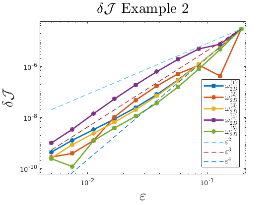
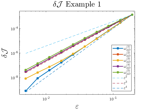
with two constants ε0=0.005{\varepsilon}_{0}=0.005 and δ=1.5\delta=1.5, and solved the perturbed PDE constraint (2.9) on a mesh which is highly refined around the point zz and evaluated the cost function to get perturbed cost function values 𝒥⁡(Ωε)\mathcal{J}(\Omega_{\varepsilon}). For all ε∈ε¯{\varepsilon}\in\underline{{\varepsilon}} and for each of the five inclusion shapes ω2​D(i)\omega_{2D}^{(i)}, we computed the quantities δ​𝒥\delta\mathcal{J} defined in (3.2). In Figure 2, it can be observed that, for each inclusion shape, δ​𝒥\delta\mathcal{J} behaves (at least) like ε3{\varepsilon}^{3}. In the case of the two inclusions ω2​D(1)\omega_{2D}^{(1)}, ω2​D(3)\omega_{2D}^{(3)} which are symmetric with respect to both the x1x_{1}- and the x2x_{2}-axes, we can even observe that δ​𝒥=𝒪⁡(ε4)\delta\mathcal{J}=\mathcal{O}({\varepsilon}^{4}). This is expected since it is known that the second term in the expansion (3.1) vanishes, d2​𝒥​(Ω,ω)​(z)=0d^{2}\mathcal{J}(\Omega,\omega)(z)=0 for this example if symmetric inclusion shapes ω\omega are considered, see e.g. [8]. In Figure 2 as well as in the subsequent Taylor test graphs, the data for ω2​D(i)\omega_{2D}^{(i)}, i>1i>1, is scaled such that they coincide with the data for ω2​D(1)\omega_{2D}^{(1)} for the largest considered value of ε{\varepsilon}. This is done for better comparison of the convergence rates.
Refer to caption
Figure 2. Numerical verification of topological asymptotic expansion (3.1) for Example 1 for five different inclusion shapes.
Refer to caption
Figure 3. Numerical verification of topological asymptotic expansion (3.1) for Example 2 for five different inclusion shapes.

We will further investigate the numerically computed topological derivative for this example in Section 4 where we will also discuss the efficient evaluation of the topological derivative in the full computational domain 𝖣\mathsf{D}.

3.1.2. Example 2: A nonlinear diffusion-convection-reaction problem in 2D

Next, we consider a more general, quasilinear setting of problem (3.3)–(3.5) where we set ud=0u_{d}=0, α~1=1\tilde{\alpha}_{1}=1, α~2=2\tilde{\alpha}_{2}=2, β~1=1\tilde{\beta}_{1}=1, β~2=2\tilde{\beta}_{2}=2, γ~=1\tilde{\gamma}=1, 𝐛1=(1,0)⊤\mathbf{b}_{1}=(1,0)^{\top}, 𝐛2=(0,1)⊤\mathbf{b}_{2}=(0,1)^{\top}, f1=1f_{1}=1, f2=2f_{2}=2, 𝐌1=(1,0)⊤\mathbf{M}_{1}=(1,0)^{\top}, 𝐌2=(0,1)⊤\mathbf{M}_{2}=(0,1)^{\top}, gN​(x1,x2)=x1​x2g_{N}(x_{1},x_{2})=x_{1}x_{2} as well as the nonlinear functions

βε​(x,|∇u​(x)|)={1x∈Ωε,β^2​(|∇u​(x)|)else,αε​(x,u⁡(x))={1x∈Ωε,u​(x)3else,\displaystyle\beta_{\varepsilon}(x,|\nabla u(x)|)=\begin{cases}1&x\in\Omega_{\varepsilon},\\ \hat{\beta}_{2}(|\nabla u(x)|)&\mbox{else},\end{cases}\qquad\alpha_{\varepsilon}(x,u(x))=\begin{cases}1&x\in\Omega_{\varepsilon},\\ u(x)^{3}&\mbox{else},\end{cases}

where β^2(s)=ν0−(ν0−200)e−s6/1000\hat{\beta}_{2}(s)=\nu_{0}-(\nu_{0}-200)e^{-s^{6}/1000} with ν0=107/(4​π)\nu_{0}=10^{7}/(4\pi). This function is sometimes used as a magentic reluctivity function in electromagnetics and satisfies the monotonicity and Lipschitz conditions which ensure existence of a unique solution to the PDE constraint. Topological derivatives for problems involving quasilinear PDE constraints are challenging from both the analytical and the numerical point of view, see e.g. [5, 6, 12, 14]. The numerical experiments depicted in Figure 3 seem to exhibit the behavior 𝒪⁡(ε3)\mathcal{O}({\varepsilon}^{3}) for all five inclusion shapes which is in accordance with (3.2) and therefore confirms the numerically computed value for the topological derivative.

3.1.3. Example 3: A linear diffusion-convection-reaction problem in 3D

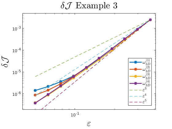
Next, we consider a linear three-dimensional version of (3.3)–(3.5) on the domain 𝖣=B⁡(𝟎,1)\mathsf{D}=B(\mathbf{0},1) with the subdomain Ω=B⁡((0,−0.7,0)⊤,0.2)\Omega=B((0,-0.7,0)^{\top},0.2). We chose the parameters ud=0u_{d}=0, α~1=1\tilde{\alpha}_{1}=1, α~2=2\tilde{\alpha}_{2}=2, β~1=β~2=0\tilde{\beta}_{1}=\tilde{\beta}_{2}=0, γ~=0\tilde{\gamma}=0, β1=1\beta_{1}=1, β2=2\beta_{2}=2, 𝐛1=𝐛2=(0,0)⊤\mathbf{b}_{1}=\mathbf{b}_{2}=(0,0)^{\top}, f1=1f_{1}=1, f2=2f_{2}=2, 𝐌1=𝐌2=(0,0)⊤\mathbf{M}_{1}=\mathbf{M}_{2}=(0,0)^{\top}, gN​(x1,x2)=x1​x2g_{N}(x_{1},x_{2})=x_{1}x_{2} and evaluate the topological derivative at the point z=(0,0.1,0)⊤z=(0,0.1,0)^{\top}. For each of the four inclusion shapes ω3​D(i)\omega_{3D}^{(i)}, i=1,2,3,4i=1,2,3,4, we solved the corresponding corrector equation (2.24) on a three-dimensional ball BRB_{R} of radius R=1000R=1000 using a tetrahedral mesh with 301116 vertices. Subsequently, we computed the topological derivative according to Section 2.5.6 and computed the quantities δ​𝒥\delta\mathcal{J} (3.2) for the vector of radius values (3.12) with ε0=0.05{\varepsilon}_{0}=0.05 and δ=1.25\delta=1.25. Figure 4 shows that the quantities δ​𝒥\delta\mathcal{J} decay at least as fast as ε4{\varepsilon}^{4} for all four inclusion shapes, which is in accordance with (3.1). The deterioration of the rates in Figure 4 can be attributed to the discretization error. We used a mesh consisting of 245177 vertices for the computational domain 𝖣\mathsf{D} which is highly refined around the point zz.

Refer to caption
Figure 4. Numerical verification of topological asymptotic expansion (3.1) for Example 3 for four different inclusion shapes.
Refer to caption
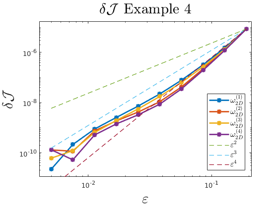
Figure 5. Numerical verification of topological asymptotic expansion (3.1) for Example 4 for four different inclusion shapes.

3.2. Elasticity

In this section, we consider vector-valued partial differential equations coming from elasticity as PDE constraints. We consider the computational domain 𝖣=(0,2)×(0,1)\mathsf{D}=(0,2)\times(0,1) which is clamped at the top left and bottom left, ΓD={(x1,x2):x1=0​ and ​x2∈[0,0.12]∪[0.88,1]}\Gamma_{D}=\{(x_{1},x_{2}):x_{1}=0\mbox{ and }x_{2}\in[0,0.12]\cup[0.88,1]\} and is subject to a downward directed force at ΓN=1×(0.45,0.55)\Gamma_{N}={1}\times(0.45,0.55). On the rest of the boundary, Γ:=∂𝖣∖(ΓD∪ΓN)\Gamma:=\partial\mathsf{D}\setminus(\Gamma_{D}\cup\Gamma_{N}), homogeneous Neumann boundary conditions are set. The domain consists of a strong material with Young’s modulus E=1000E=1000, and a very weak material which mimicks void inside Ω=B⁡((0.5,0.5)⊤,0.3)∪B⁡((1.8,0.25)⊤,0.1)∪B⁡((1.8,0.75)⊤,0.1)\Omega=B((0.5,0.5)^{\top},0.3)\cup B((1.8,0.25)^{\top},0.1)\cup B((1.8,0.75)^{\top},0.1) where E=0.1E=0.1, see Figure 6(a). The Poisson ratio is set to ν=13\nu=\frac{1}{3} in both subdomains. We consider the problem to minimize the compliance of the structure which is subject to self-weight as well as an external force acting on the boundary ΓN\Gamma_{N}. The problem reads

min Ω​J​(u,Ω):=12​∫𝖣SΩ​(𝒟​u):𝒟​u​d​x\displaystyle\underset{\Omega}{\mbox{min }}J(u,\Omega):=\frac{1}{2}\int_{\mathsf{D}}S_{\Omega}(\mathcal{D}u):\mathcal{D}u\;\mbox{d}x (3.13)

such that

u∈HΓD1​(𝖣)d:∫𝖣SΩ​(𝒟​u):𝒟​ψ​d​x=\displaystyle u\in H^{1}_{\Gamma_{D}}(\mathsf{D})^{d}:\int_{\mathsf{D}}S_{\Omega}(\mathcal{D}u):\mathcal{D}\psi\;\mbox{d}x= ∫𝖣fΩ⋅ψ​d​x+∫ΓNgN⋅ψ​d​S\displaystyle\int_{\mathsf{D}}f_{\Omega}\cdot\psi\;\mbox{d}x+\int_{\Gamma_{N}}g_{N}\cdot\psi\;\mbox{d}S (3.14)

for all ψ∈HΓD1​(𝖣)d\psi\in H^{1}_{\Gamma_{D}}(\mathsf{D})^{d}, where SΩ:𝐑d×d→𝐑d×dS_{\Omega}:{\mathbf{R}}^{d\times d}\rightarrow{\mathbf{R}}^{d\times d} represents a stress tensor and fΩf_{\Omega} is a piecewise constant vector function. Also this problem fits into the framework considered in Section 2 by setting

jΩ​(x,u⁡(x),𝒟​u​(x))=\displaystyle j^{\Omega}(x,u(x),\mathcal{D}u(x))= 12​SΩ​(𝒟​u​(x)):𝒟​u​(x),\displaystyle\frac{1}{2}S_{\Omega}(\mathcal{D}u(x)):\mathcal{D}u(x),
A1Ω​(x,u⁡(x),𝒟​u​(x))=\displaystyle A_{1}^{\Omega}(x,u(x),\mathcal{D}u(x))= 0,\displaystyle 0,
A2Ω​(x,u⁡(x),𝒟​u​(x))=\displaystyle A_{2}^{\Omega}(x,u(x),\mathcal{D}u(x))= SΩ​(𝒟​u​(x)),\displaystyle S_{\Omega}(\mathcal{D}u(x)),
F1Ω​(x)=\displaystyle F_{1}^{\Omega}(x)= fΩ​(x),\displaystyle f_{\Omega}(x),
F2Ω​(x)=\displaystyle F_{2}^{\Omega}(x)= 0.\displaystyle 0.
Refer to caption Refer to caption
(a) (b)
Refer to caption Refer to caption
(c) (d)
Figure 6. (a) Computational domain 𝖣\mathsf{D} with subdomain Ω\Omega for Examples 4 and 5. (b) Solution to linear state equation of Example 4 (undeformed). (c) Solution to nonlinear state equation of Example 5 in deformed configuration. (d) Deformed domain of Example 5.

3.2.1. Example 4: Linear elasticity in 2D

We consider problem (3.13)–(3.14) for the two-dimensional cantilever example introduced above under a linear stress-strain relation,

SΩ​(𝒟​u)=2​μΩ​e​(u)+λΩ​T​r​(e⁡(u))​I2\displaystyle S_{\Omega}(\mathcal{D}u)=2\mu_{\Omega}e(u)+\lambda_{\Omega}Tr(e(u))I_{2} (3.15)

with the piecewise defined Lamé coefficients

μΩ​(x)=χΩ​(x)​μ1+χ𝖣∖Ω​(x)​μ2,λΩ​(x)=χΩ​(x)​λ1+χ𝖣∖Ω​(x)​λ2,\displaystyle\mu_{\Omega}(x)=\chi_{\Omega}(x)\mu_{1}+\chi_{\mathsf{D}\setminus\Omega}(x)\mu_{2},\qquad\lambda_{\Omega}(x)=\chi_{\Omega}(x)\lambda_{1}+\chi_{\mathsf{D}\setminus\Omega}(x)\lambda_{2},

corresponding to Young’s modulus E2=1000E_{2}=1000, E1=0.1E_{1}=0.1 and Poisson ratio ν2=ν1=13\nu_{2}=\nu_{1}=\frac{1}{3}, i.e.,

μi=Ei​12​(1+νi)λi=Ei​νi(1+νi)​(1−2​νi),for ​i=1,2.\displaystyle\mu_{i}=E_{i}\frac{1}{2(1+\nu_{i})}\qquad\lambda_{i}=E_{i}\frac{\nu_{i}}{(1+\nu_{i})(1-2\nu_{i})},\quad\mbox{for }i=1,2. (3.16)

Here, e⁡(u)=12​(𝒟​u+𝒟​u⊤)e(u)=\frac{1}{2}(\mathcal{D}u+\mathcal{D}u^{\top}) denotes the linearized strain tensor, T​r​(A)Tr(A) denotes the trace of a matrix AA and I2I_{2} denotes the two-dimensional identity matrix. Moreover, in this example we neglect self-weight, fΩ=0f_{\Omega}=0, and consider the external load gN=(0,−1)⊤g_{N}=(0,-1)^{\top} acting on ΓN\Gamma_{N}.

We computed the unperturbed state and adjoint on a mesh with about 150 000 vertices (resulting in about 300 000 degrees of freedom) which is highly refined around the point z=(1.2,0.5)⊤z=(1.2,0.5)^{\top} for which we compute and verify the topological derivative. We solve the corrector equation (2.24) with four considered two-dimensional inclusion shapes ω2​D(i)\omega_{2D}^{(i)}, i=1,…​4i=1,\dots 4 where we replace the unbounded domain 𝐑d{\mathbf{R}}^{d} by the large, but bounded domain BR=B⁡(𝟎,R)B_{R}=B(\mathbf{0},R) with R=1000R=1000 using a mesh with about 370 000 vertices. We again compute the quantities δ​𝒥\delta\mathcal{J} defined in (3.2) for a range of values for the inclusion radius ε{\varepsilon} (3.12) with ε0=0.005{\varepsilon}_{0}=0.005 and δ=1.5\delta=1.5. The behavior of δ​𝒥\delta\mathcal{J} for these five inclusion shapes can be seen in Figure 5 where we can again observe the behavior δ​𝒥=𝒪⁡(ε3)\delta\mathcal{J}=\mathcal{O}({\varepsilon}^{3}) for all five inclusion shapes.

3.2.2. Example 5: Nonlinear elasticity in 2D

Finally, we consider problem (3.13)–(3.14) with the nonlinear St. Venant-Kirchhoff material

SΩ​(𝒟​u):=(I2+𝒟​u)​[λΩ​Tr​(12​(C⁡(𝒟​u)−I2))​I2+μΩ​(C⁡(𝒟​u)−I2)],\displaystyle S_{\Omega}(\mathcal{D}u):=(I_{2}+\mathcal{D}u)\left[\lambda_{\Omega}\mbox{Tr}(\frac{1}{2}(C(\mathcal{D}u)-I_{2}))I_{2}+\mu_{\Omega}(C(\mathcal{D}u)-I_{2})\right], (3.17)

with C⁡(𝒟​u):=(I2+𝒟​u)⊤​(I2+𝒟​u)=I2+𝒟​u+𝒟​u⊤+𝒟​u⊤​𝒟​uC(\mathcal{D}u):=(I_{2}+\mathcal{D}u)^{\top}(I_{2}+\mathcal{D}u)=I_{2}+\mathcal{D}u+\mathcal{D}u^{\top}+\mathcal{D}u^{\top}\mathcal{D}u, and λΩ=χΩ​λ1+χ𝖣∖Ω​λ2\lambda_{\Omega}=\chi_{\Omega}\lambda_{1}+\chi_{\mathsf{D}\setminus\Omega}\lambda_{2}, μΩ=χΩ​μ1+χ𝖣∖Ω​μ2\mu_{\Omega}=\chi_{\Omega}\mu_{1}+\chi_{\mathsf{D}\setminus\Omega}\mu_{2} with E2=1000E_{2}=1000, E1=0.1E_{1}=0.1 and ν2=ν1=0.3\nu_{2}=\nu_{1}=0.3 and λ1,λ2,μ1,μ2\lambda_{1},\lambda_{2},\mu_{1},\mu_{2} defined as in (3.16). Here we use the larger external force gN=(0,−20)⊤g_{N}=(0,-20)^{\top} acting on ΓN\Gamma_{N} and also mimic self-weight with f2=(0,−5)⊤f_{2}=(0,-5)^{\top}, f1=0f_{1}=0.

For solving the state, adjoint and corrector equations, we use the same meshes as in Example 4. For solving the nonlinear state equation (2.4) we use a load stepping scheme with Nl​s=20N_{ls}=20 load steps where we gradually increase the loads given by f2f_{2} and gNg_{N} until they reach their full values given above, i.e., we solve (2.4) with the data given above and

f2=kNl​s​(0−5)gN=kNl​s​(0−20)\displaystyle f_{2}=\frac{k}{N_{ls}}\left(\begin{array}[]{c}0\\ -5\end{array}\right)\qquad g_{N}=\frac{k}{N_{ls}}\left(\begin{array}[]{c}0\\ -20\end{array}\right)

for k=1,…​Nl​sk=1,\dots N_{ls}. For each load step, we use Newton’s method to solve (2.4) for the given loads. The solution to the nonlinear state equation in deformed configuration can be seen in Figure 6(c) and the deformed domain in Figure 6(d). Moreover, we solve the corrector equation (2.24) by means of a damped Newton method with a very conservative damping factor of 0.0020.002.

We performed a Taylor test by computing the quantities δ​𝒥\delta\mathcal{J} for the four inclusion shapes ω2​D(i)\omega_{2D}^{(i)}, i=1,2,3,4i=1,2,3,4, using the same parameters ε¯\underline{{\varepsilon}} as in Example 4. Figure 7 shows that δ​𝒥\delta\mathcal{J} decays at least as fast as ε3{\varepsilon}^{3} which confirms the topologcial asymptotic expansion (3.1).
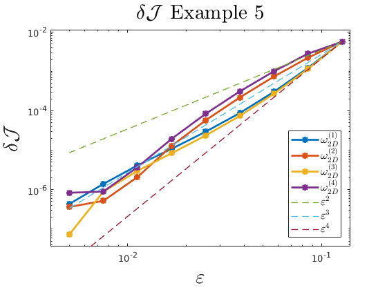
Refer to caption
Figure 7. Numerical verification of topological asymptotic expansion (3.1) for Example 5 for four different inclusion shapes.

4. On the efficient evaluation of topological derivatives in the full domain

In Section 3, we applied the systematic procedure for the computation of topological derivatives introduced in Section 2 to different model problems involving linear and nonlinear PDE constraints in two and three space dimensions. Moreover we verified the obtained values by Taylor tests. However, looking at the formulas of Section 2.5.6, it can be seen that the evaluation of the topological derivative at a spatial point zz requires the solution of the corrector equation (2.24). On the other hand, in order to employ an optimization algorithm, one usually is interested in the topological derivative in the full design domain. Of course, solving (2.24) for every spatial point in the design domain (or every element of a mesh) is prohibitively expensive.

In the following, we show how, for linear or semilinear PDE constraints, the corresponding solution KK can be obtained as a linear combination of some functions which can be precomputed. Note that, since we assume the PDE constraint to be linear or semilinear, both A2inA_{2}^{\text{in}} and A2o​u​tA_{2}^{out} are linear with respect to the third argument 𝒟​u\mathcal{D}u and constant with respect to the second argument uu, i.e., there exist a2in​(z),a2o​u​t​(z)a_{2}^{\text{in}}(z),a_{2}^{out}(z) such that

A2in​(z,u0​(z),𝒟​u0​(z))=a2in​(z)​𝒟​u0​(z)andA2o​u​t​(z,u0​(z),𝒟​u0​(z))=a2o​u​t​(z)​𝒟​u0​(z).\displaystyle A_{2}^{\text{in}}(z,u_{0}(z),\mathcal{D}u_{0}(z))=a_{2}^{\text{in}}(z)\mathcal{D}u_{0}(z)\quad\mbox{and}\quad A_{2}^{out}(z,u_{0}(z),\mathcal{D}u_{0}(z))=a_{2}^{out}(z)\mathcal{D}u_{0}(z).

We introduce the notation

a2ω​(z,𝒟​u0​(z)):=χω​(x)​a2in​(z)​𝒟​u0​(z)+χ𝐑d∖ω​(x)​a2o​u​t​(z)​𝒟​u0​(z).\displaystyle a_{2}^{\omega}(z,\mathcal{D}u_{0}(z)):=\chi_{\omega}(x)a_{2}^{\text{in}}(z)\mathcal{D}u_{0}(z)+\chi_{{\mathbf{R}}^{d}\setminus\omega}(x)a_{2}^{out}(z)\mathcal{D}u_{0}(z).

Now let K^\hat{K} be the solution to

∫𝐑d\displaystyle\int_{{\mathbf{R}}^{d}} a2ω​(z,𝒟​K^):𝒟​ψ​𝑑x=∫ω(F2in−F2o​u​t)​(z):𝒟​ψ​𝑑x\displaystyle a_{2}^{\omega}(z,\mathcal{D}\hat{K}):\mathcal{D}\psi\;dx=\int_{\omega}(F_{2}^{\text{in}}-F_{2}^{out})(z):\mathcal{D}\psi\;dx (4.1)

for all ψ\psi and, for i∈{1,…,m}i\in\{1,\dots,m\}, j∈{1,…,d}j\in\{1,\dots,d\}, let K~ei​j\tilde{K}_{e_{ij}} be the solution to

∫𝐑da2ω​(z,𝒟​K~ei​j):𝒟​ψ​d​x=−∫ω(a2in−a2o​u​t)(z)ei​j:𝒟ψdx\displaystyle\begin{aligned} \int_{{\mathbf{R}}^{d}}&a_{2}^{\omega}(z,\mathcal{D}\tilde{K}_{e_{ij}}):\mathcal{D}\psi\;dx&=-\int_{\omega}(a_{2}^{\text{in}}-a_{2}^{out})(z)e_{ij}:\mathcal{D}\psi\;dx\end{aligned} (4.2)

for all ψ\psi. Here ei​j∈𝐑m×de_{ij}\in{\mathbf{R}}^{m\times d} denotes the unit basis element with the value 11 at the position (i,j)(i,j) and the value 00 else.

These considerations immediately yield the following lemma.

Lemma 1.

Assume that the PDE constraint (2.4) is linear or semilinear and let 𝒟​u0​(z)∈𝐑m×d\mathcal{D}u_{0}(z)\in{\mathbf{R}}^{m\times d} be given. Then the solution KK to (2.24) is given as the linear combination

K=K^+∑i=1m∑j=1d(a2in−a2o​u​t)​(z)​𝒟​u0​(z)​[i,j]​K~ei​j\displaystyle K=\hat{K}+\sum_{i=1}^{m}\sum_{j=1}^{d}(a_{2}^{\text{in}}-a_{2}^{out})(z)\mathcal{D}u_{0}(z)[i,j]\,\tilde{K}_{e_{ij}} (4.3)

with K^\hat{K} and K~ei​j\tilde{K}_{e_{ij}} given in (4.1) and (4.2), respectively.

Using Lemma 1 it is possible to compute the solution KK of (2.24) for any value of 𝒟​u0​(z)\mathcal{D}u_{0}(z) by linear combination once the m​d+1md+1 functions K^\hat{K}, K~ei​j\tilde{K}_{e_{ij}} have been computed. By integration over ω\omega or 𝐑d{\mathbf{R}}^{d} (which is numerically approximated by B⁡(𝟎,R)B(\mathbf{0},R) with R=1000R=1000), the topological derivative can then be approximately evaluated at every point without having to solve an additional boundary value problem.

In the case of Example 1 (Section 3.1.1), it follows from 𝐌1=𝐌2=(0,0)⊤\mathbf{M}_{1}=\mathbf{M}_{2}=(0,0)^{\top} that K^=0\hat{K}=0. Since m=1m=1, d=2d=2, we need to precompute the solutions to (4.2) for the two unit vectors in 𝐑2{\mathbf{R}}^{2} and can obtain the solution KK to (2.24) by Lemma 1. The solutions K~e11\tilde{K}_{e_{11}} and K~e12\tilde{K}_{e_{12}} to (4.2) with 𝐑d{\mathbf{R}}^{d} replaced by B⁡(𝟎,1000)B(\mathbf{0},1000) are depicted in Figure 8.

Refer to caption Refer to caption
Figure 8. Solutions to (4.2) for e11=(1,0)⊤e_{11}=(1,0)^{\top} (left) and e12=(0,1)⊤e_{12}=(0,1)^{\top} (right).

Next, we chose a (comparably coarse) mesh with only background material, i.e. Ω=∅\Omega=\emptyset, and numerically computed the topological derivative for the centroid of every triangular element by evaluating the formulas of Section 2.5.6. Also here, integrals over 𝐑d{\mathbf{R}}^{d} were approximated by integrals over the large, but bounded ball B⁡(𝟎,1000)B(\mathbf{0},1000). A comparison of the obtained results with the analytical formula for the topological derivative given in (3.11) showed good accordance, see Figure 9.

Refer to caption Refer to caption Refer to caption
Figure 9. Left: Numerically computed topological derivative for Example 1. Center: Analytical formula (3.11). Right: Difference between numerical and analytical formulas. Observe the different orders of magnitude.
Remark 4.

The procedure described in this section is still computationally expensive since it involves the numerical computation of several integrals over ω\omega and B⁡(𝟎,1000)B(\mathbf{0},1000) for each topological derivative evaluation.

We remark that in many cases it is possible to exploit the (affine) linearity of the topological derivative d​𝒥d\mathcal{J} (2.23) with respect to the adjoint state as well as some rotational symmetry property of KK with respect to 𝒟​u0​(z)\mathcal{D}u_{0}(z) to directly precompute the topological derivative d​𝒥d\mathcal{J} for some basis elements and to obtain the full topological derivative as a linear combination of these values. We remark that such a procedure – if applicable – can be computationally cheaper and allow for the use of the obtained formulas in iterative topology optimization algorithms, see e.g. [6, 14] for more details.

Conclusion and Outlook

We have illustrated a systematic way of computing topological derivatives for a large class of PDE-constrained topology optimization problems. Using automated differentiation in NGSolve, it was possible to compute all potential terms of the topological derivative for an abstract problem class. We showed the effectivity of the method in several linear and nonlinear model problems and verified the topological derivative formulas by computing the values of the topological asymptotic expansion that should be satisfied by the topological derivative.

The presented work can be extended in several directions. On the one hand, we only considered problems posed in an H1H^{1} setting. We remark that the same procedure is possible for any differential operator 𝒟\mathcal{D} that scales as (𝒟​φ)∘Tε=1ε​𝒟​(φ∘Tε)(\mathcal{D}\varphi)\circ T_{\varepsilon}=\frac{1}{{\varepsilon}}\mathcal{D}(\varphi\circ T_{\varepsilon}). In particular, this also includes the c​u​r​lcurl operator, thus also allowing to treat H⁡(c​u​r​l)H(curl) problems as they arise in electromagnetics [14]. Moreover, for some linear problems, the computational effort for solving the corrector equation (2.24) could be reduced by employing a boundary element method rather than a finite element method on an approximation of the unbounded domain. Finally, a further topic of future research is the numerical analysis of the topological derivative with respect to mesh sizes in the bounded domain 𝖣\mathsf{D} and in the blown-up domain BRB_{R} as well as with respect to the radius RR of the large domain.

References

  • [1] G. Allaire and F. Jouve. Coupling the level set method and the topological gradient in structural optimization. In Springer, editor, IUTAM Symposium on Topological Design Optimization of Structures, Machines and Materials, pages 3–12, 2006.
  • [2] H. Ammari and H. Kang. Polarization and Moment Tensors. Springer-Verlag New York, 2007.
  • [3] S. Amstutz. Sensitivity analysis with respect to a local perturbation of the material property. Asymptotic analysis, 49(1), 2006.
  • [4] S. Amstutz and H. Andrä. A new algorithm for topology optimization using a level-set method. Journal of Computational Physics, 216(2):573–588, 2006.
  • [5] S. Amstutz and A. Bonnafé. Topological derivatives for a class of quasilinear elliptic equations. Journal de Mathématiques Pures et Appliquées, 107(4):367–408, 2017.
  • [6] S. Amstutz and P. Gangl. Topological derivative for the nonlinear magnetostatic problem. Electron. Trans. Numer. Anal., 51:169–218, 2019.
  • [7] S. Amstutz, A.A. Novotny, and N. Van Goethem. Topological sensitivity analysis for elliptic differential operators of order 2m. Journal of Differential Equations, 256(4):1735–1770, 2014.
  • [8] P. Baumann and K. Sturm. Adjoint based methods for the computation of higher order topological derivatives with an application to linear elasticity. arXiv, 2021.
  • [9] M. Burger, B. Hackl, and W. Ring. Incorporating topological derivatives into level set methods. Journal of Computational Physics, 194(1):344–362, 2004.
  • [10] M.C. Delfour. Control, shape, and topological derivatives via minimax differentiability of lagrangians. In Springer INdAM Series, pages 137–164. Springer International Publishing, 2018.
  • [11] H. A. Eschenauer, V. V. Kobelev, and A. Schumacher. Bubble method for topology and shape optimization of structures. Structural optimization, 8(1):42–51, 1994.
  • [12] P. Gangl and K. Sturm. A simplified derivation technique of topological derivatives for quasi-linear transmission problems. ESAIM Control Optim. Calc. Var., 26:Paper No. 106, 20, 2020.
  • [13] P. Gangl and K. Sturm. Topological derivative for PDEs on surfaces, 2020.
  • [14] P. Gangl and K. Sturm. Asymptotic analysis and topological derivative for 3d quasi-linear magnetostatics. ESAIM: Mathematical Modelling and Numerical Analysis, 55:S853–S875, 2021.
  • [15] P. Gangl and K. Sturm. Supplementary code for article ”Automated computation of topological derivatives with application to nonlinear elasticity and reaction-diffusion problems”, 2021. https://doi.org/10.5281/zenodo.5118379.
  • [16] P. Gangl, K. Sturm, M. Neunteufel, and J. Schöberl. Fully and semi-automated shape differentiation in NGSolve. Structural and Multidisciplinary Optimization, 63(3):1579–1607, November 2020.
  • [17] S. Garreau, P. Guillaume, and M. Masmoudi. The Topological Asymptotic for PDE Systems: The Elasticity Case. SIAM Journal on Control and Optimization, 39(6):1756–1778, 2001.
  • [18] M. Hintermüller. Fast level set based algorithms using shape and topological sensitivity information. Control and Cybernetics, 34(1), 2005.
  • [19] M. Hintermüller, A. Laurain, and A. A. Novotny. Second-order topological expansion for electrical impedance tomography. Advances in Computational Mathematics, 36(2):235–265, 2012.
  • [20] A. A. Novotny and J. Sokołowski. Topological derivatives in shape optimization. Interaction of Mechanics and Mathematics. Springer, Heidelberg, 2013.
  • [21] J. Schöberl. C++11 implementation of finite elements in NGSolve. Technical Report 30, Institute for Analysis and Scientific Computing, Vienna University of Technology, 2014.
  • [22] J. Sokołowski and A. Zochowski. On the topological derivative in shape optimization. SIAM Journal on Control and Optimization, 37(4):1251–1272, 1999.
  • [23] K. Sturm. Topological sensitivities via a Lagrangian approach for semilinear problems. Nonlinearity, 33(9):4310–4337, jul 2020.