Towards Plug-and-Play Visual Graph Query Interfaces: Data-driven Canned Pattern Selection for Large Networks
Abstract.
Canned patterns (i.e., small subgraph patterns) in visual graph query interfaces (a.k.a gui) facilitate efficient query formulation by enabling pattern-at-a-time construction mode. However, existing guis for querying large networks either do not expose any canned patterns or if they do then they are typically selected manually based on domain knowledge. Unfortunately, manual generation of canned patterns is not only labor intensive but may also lack diversity for supporting efficient visual formulation of a wide range of subgraph queries. In this paper, we present a novel generic and extensible framework called Tattoo that takes a data-driven approach to automatically selecting canned patterns for a gui from large networks. Specifically, it first decomposes the underlying network into truss-infested and truss-oblivious regions. Then candidate canned patterns capturing different real-world query topologies are generated from these regions. Canned patterns based on a user-specified plug are then selected for the gui from these candidates by maximizing coverage and diversity, and by minimizing the cognitive load of the pattern set. Experimental studies with real-world datasets demonstrate the benefits of Tattoo. Importantly, this work takes a concrete step towards realizing plug-and-play visual graph query interfaces for large networks.
1. Introduction
A recent survey (SM+17) revealed that graph query languages and usability are considered as some of the top challenges for graph processing. A common starting point for addressing these challenges is the deployment of a visual query interface (a.k.a gui) that can enable an end user to draw a graph query interactively by utilizing direct-manipulation (SP) and visualize the result matches effectively (PH+17; bloom). A useful component of such a gui is a panel containing a set of canned patterns (i.e., small subgraphs) which is beneficial to visual querying in at least three possible ways (bhowmick2016; catapult; midas). First, it can potentially decrease the time taken to visually construct a query by facilitating pattern-at-a-time query mode (i.e., construct multiple nodes and edges by performing a single click-and-drag action) in lieu of edge-at-a-time mode. Second, it can facilitate “bottom-up” search when a user does not have upfront knowledge of what to search for. Third, canned patterns (patterns for brevity) may alleviate user frustration of repeated edge construction especially for larger queries.

Example 1.1.
Consider the real-world subgraph query in Figure 1 from bsbm (bsbm) (Query ). Suppose Wei, a non-programmer, wishes to formulate it using a gui containing a set of canned patterns (a subset of patterns is shown). Specifically, he may drag and drop and on the Query Canvas, merge the yellow vertex of with the center vertex of , add a vertex and connect it with the grey vertex of . Finally, Wei can assign appropriate vertex labels. Observe that it requires five steps to construct the topology. On the other hand, if Wei takes an edge-at-a-time approach to construct the query, it would require 23 steps. Clearly, canned patterns enable more efficient (i.e., fewer number of steps or lesser time) formulation of the query.
It is worth noting that Wei may not necessarily have the complete query structure “in his head” during query formulation. He may find interesting while browsing the pattern set, which may initiate his bottom-up search leading to the query. Clearly, without the existence of a pattern set, such bottom-up search would be infeasible in practice.
Data-driven selection of relevant canned patterns for a gui (e.g., , , in Fig. 1) is important to facilitate efficient query formulation (catapult; bhowmick2016). In particular, data-driven selection paves the way for plug-and-play visual graph query interfaces, which are like a plug-and-play device that can be plugged into any kind of socket (i.e., graph data) and used. A plug-and-play gui is dynamically built from a high-level specification of canned pattern properties known as the plug (detailed in Section 3). Specifically, given a network and a plug , the gui is automatically constructed by populating its various components (e.g., node/edge attributes, canned patterns) from without the need for manual gui coding. This enhances portability and maintainability of guis across different data sources (bhowmick2016).
In this paper, we present a novel framework called Tattoo (daTa-driven cAnned paTtern selecTiOn from netwOrks) that takes a data-driven approach to the canned pattern selection (cps) problem for large networks. Given a network , a user-specified plug specification which is the number of canned patterns to display and their minimum and maximum permissible sizes, Tattoo automatically selects canned patterns from that satisfy .
The cps problem is technically challenging. First, it is a NP-hard problem (catapult). Second, the availability of query logs can facilitate the selection of relevant patterns as they provide rich information of past queries. In practice, however, such information is often publicly unavailable (e.g., none of the networks in snap (snap) reveal query logs) due to privacy and legal reasons. Hence, we cannot realistically assume the availability of query logs to select patterns. Furthermore, users may demand a gui prior to querying a network. Hence, there may not exist any query log prior to the creation of a visual query interface. Third, it is paramount to find unlabeled patterns (e.g., Example 1.1) that are potentially useful for query formulation (detailed in Sec. 4). However, the selection of such patterns is challenging as there is an exponential number of them in a large network. Fourth, these selected patterns should not only be topologically diverse so that they are useful for a wide variety of queries but they should also impose low cognitive load (i.e., mental load to visually interpret a pattern’s edge relationships to determine if it is useful for a query) on users. In particular, large graphs overload the human perception and cognitive systems, resulting in poor performance of tasks such as identifying edge relationships (huang2009; YA+18).
At this point, a keen reader may wonder why building blocks of real-world networks (e.g., paths of length , triangle patterns) (wang2003; milo2002) cannot be simply utilized as canned patterns since they have high coverage and low cognitive load. However, it may take a larger number of steps to formulate a variety of queries using these patterns due to their small size. For instance, reconsider Example 1.1. Suppose the pattern set consists of an edge, a path of length 2 (i.e., 2-path), a triangle, and a rectangle. In this case, may be formulated by dragging and dropping the rectangle once, the 2-path three times, construction of a single node and two edges, along with three node mergers. That is, it takes 10 steps altogether, which is more than using the patterns in Figure 1. Furthermore, these patterns do not expose “interesting” substructures to facilitate bottom-up search as they occur in almost all large real-world networks.

Tattoo addresses the aforementioned challenges as follows. It exploits a recent analysis of real-world query logs (Bonifati2017) to classify topologies of canned patterns into categories that are consistent with the topologies of real-world queries (detailed in Section 5). This enables us to reach a middle ground where Tattoo does not need to be restricted by the availability of query logs but yet exploit topological characteristics of real-world queries to guide the selection process. Next, it realizes a novel and efficient candidate canned pattern generation technique based on the classified topologies to identify potentially useful patterns. Lastly, canned patterns are selected from these candidates for display on the gui based on a novel pattern set score that is sensitive to coverage, diversity, and cognitive load of patterns. Specifically, we leverage recent progress in the algorithm community to propose a selection algorithm that guarantees -approximation (buchbinder2014). Figure 2 depicts an overview of the Tattoo framework. Experiments with several real-world large networks and users reveal that Tattoo can select canned patterns within few minutes. Importantly, these patterns can reduce the number of steps taken to formulate a subgraph query and query formulation time by up to 9.7X and 18X, respectively, compared to several baseline strategies.
In summary, this paper makes the following contributions: (1) We describe Tattoo, an end-to-end canned pattern selection framework for any plug-and-play visual graph query interface for large networks independent of domains and data sources. A video of a plug-and-play interface that incorporates Tattoo can be viewed at https://youtu.be/sL0yHV1eEPw. (2) We formally introduce the cps problem for large networks (Sec. 4) and present a novel categorization of potentially useful canned patterns in Section 5. (3) We present an efficient solution to select canned patterns for a gui (Sec. 6 - 7). Specifically, we present a novel candidate pattern generation framework that is grounded on topologies of real-world subgraph queries. Furthermore, for the first time in graph querying literature, we utilize the recent technique in (buchbinder2014) from the algorithm community to select canned patterns with good theoretical quality guarantees. (4) Using real-world networks, we show the superiority of our proposed framework compared to several baselines (Sec. 8).
Proofs of theorems and lemmas are provided in Appendix A.
2. Related Work
Most germane to our work is our prior efforts on data-driven construction of visual graph query interfaces in (zhang2015davinci; catapult; kai2020). The work in (midas) focuses on the maintenance of canned patterns for evolving data graphs. Our work differs from these efforts in the following ways. First, we focus on selecting unlabelled canned patterns from large networks in contrast to labelled patterns from a collection of small- or medium-sized data graphs in (zhang2015davinci; catapult; kai2020; midas). Specifically, existing efforts such as Catapult (catapult) first partitions a collection of data graphs into a set of clusters and summarizes each cluster to a cluster summary graph (csg). Then, it selects the canned patterns with the aforementioned characteristics from these csgs using a weighted random walk approach. This clustering-based approach is prohibitively expensive for large networks as detailed in Sec. 8. Second, these approaches do not exploit characteristics of real-world subgraph queries for selecting canned patterns. In contrast, we utilize topological characteristics of real-world queries to guide our solution design. Third, we present a novel real-world query topology-aware candidate pattern generation technique and a selection technique that provides quality guarantee. No theoretical guarantee is provided in (zhang2015davinci; catapult; kai2020) for selecting canned patterns. Lastly, as detailed in Sec. 7, the computation of pattern score to assess the quality of canned patterns is different as the computation of cognitive load and diversity is different from (catapult) due to the nature of large networks. Furthermore, in this work we provide a theoretical analysis of the pattern score.
Motif discovery techniques (gurukar2015; milo2002) do not consider diversity and cognitive load. Sizes of these motifs are generally bounded in the range of [3-7] in real applications (gurukar2015; milo2002). For the same reason, it is difficult to use graphlets (przulj2004; hocevar2014; ahmed2015) as patterns. Also, frequent subgraphs (dhiman2016) may not constitute good canned patterns (bhowmick2016) and are prohibitively expensive to compute for large networks (detailed in Sec. 8).
3. Background
We first introduce several graph terminologies that we shall be using subsequently. Next, we formally define the notion of plugs. Finally, we briefly describe the desirable characteristics of canned patterns as introduced in (catapult).
3.1. Terminology
We denote a graph or network as , where is a set of nodes/vertices and is a set of edges. Vertices and edges can have labels as attributes. The size of is defined as . The degree of a vertex is denoted as . In this paper, we assume that is an undirected, unweighted graph with labeled vertices.
A triangle is a cycle of length 3 in . The support of an edge (denoted by ) is the number of triangles in containing and (voegele2017). is a subgraph of (denoted by ) if and . Consider another graph where . and are isomorphic if there exists a bijection such that iff . Further, there exists a subgraph isomorphism from to a graph if contains a subgraph that is isomorphic to . We refer to as the embedding of in .
Given , the -truss of is the largest subgraph of in which every edge is contained in at least triangles within the subgraph. A 2-truss is simply itself. We define the trussness of an edge as where is the -truss in . Further, denotes the maximum trussness.
3.2. Plugs
Recall that data-driven selection of canned patterns facilitates the construction of a plug-and-play visual graph query interface. A plug is a high-level specification of the patterns in a gui. Given the specification, Tattoo dynamically generates the canned patterns satisfying it from the underlying network. Formally, it is defined as follows.
Definition 3.1.
[Plug] Given a network and a gui , a plug where (resp. ) is the minimum (resp. maximum) size of a pattern, is the number of patterns to be displayed on .
Essentially a plug11 1 Additional constraint on the distribution of the patterns which is application specific can be included in the plug. is a collection of attribute-value pairs that specifies the high-level content of a canned pattern panel in a gui. For example, is a plug. Accordingly, the minimum and maximum sizes of patterns in are 3 and 15, respectively, and the total number of patterns to be displayed is 30. Observe that there can be multiple plugs for as well. Similarly, the same plug can be used for different . Hence, different guis can be constructed by different plug specifications.
A plug should possess the following properties. (a) Data independence - A plug should not depend upon a specific network (i.e., socket). The specification of plug enables this by not admitting any network-specific information. Observe that this property is important for plug-and-play interfaces as a plug can be used on different network data across different application domains. (b) Able to select canned patterns with the required specifications - The resulting canned pattern selection mechanism should select patterns exactly as specified by the plug.
3.3. Characteristics of Canned Patterns
Since it is impractical to display a large number of patterns in a visual graph query interface , the number of patterns should be small and satisfy certain desirable characteristics as introduced in (catapult).
High coverage. A pattern covers if contains a subgraph that is isomorphic to . Since may have many embeddings in , the pattern set should ideally cover as large portion of as possible. Then a large number of subgraph queries on can be constructed by utilizing .
High diversity. High coverage of patterns is insufficient to facilitate efficient visual query formulation (catapult). In order to make efficient use of the limited display space on , should be structurally diverse to serve a variety of queries. This also facilitates bottom-up search where a user gets a bird’s-eye view of the diverse substructures in .
Low cognitive load. Cognitive load refers to the memory demand or mental effort required to perform a given task (huang2009). A topologically complex pattern may demand substantial cognitive effort from an end user to decide if it can aid in her query formulation (catapult). Hence, it is desirable for the canned patterns in to impose low cognitive load on an end user to make browsing and selecting relevant patterns cognitively efficient during visual query formulation.
4. The CPS Problem
Given a data graph or network , a visual graph query interface and a user-specified plug , the goal of the canned pattern selection (cps) problem is to select a set of unlabelled patterns for display on , which satisfies the specifications in and optimizes coverage, diversity and cognitive load of .
Observe that our cps problem differs from (catapult) in two key ways. First, we focus on a single large network instead of a large collection of small- or medium-sized data graphs. Second, we select unlabelled patterns instead of labelled ones. In large networks, a subgraph query may not always contain labels on its vertices or edges. Specifically, unlabelled query graphs are formulated in the subgraph enumeration problem (AFU13) whereas query graphs are labelled in the subgraph matching problem (SL20). Hence, by selecting unlabelled patterns Tattoo facilitates visual formulation of both these categories of queries. In particular, one may simply drag-and-drop specific vertex/edge labels from the Attribute panel of a gui to add labels to the vertices/edges of a pattern (e.g., Example 1).
We now formally define the cps problem addressed in this paper. We begin by introducing coverage, diversity, and cognitive load of canned patterns. Let be a bag of subgraphs in isomorphic to (i.e., embeddings of ) where vertex labels in and are assumed to be the same and . We say an edge is covered by . The coverage of is given as . Similarly, (i.e., ) where every is covered by at least one . Since is constant for a given , coverage can be rewritten as and . The diversity of w.r.t to is the inverse of similarity of . In particular, the similarity of a set of canned patterns is denoted as where is the similarity between patterns and (detailed in Sec. 7). Finally, we measure cognitive load of (denoted by ) based on the size, density, and edge crossings in (detailed in Sec. 7) as a user tends to spend more time identifying relationships between vertices in denser graphs with more edge crossings (huang2009; huang2010; YA+18). The cognitive load of (i.e., ) is given as .
Definition 4.1.
[CPS Problem] Given a network , a gui , and a plug , the goal of canned pattern selection (CPS) problem is to find a set of unlabelled canned patterns from that satisfies
| (1) | ||||
where is the solution; is the feasible set of canned pattern sets in ; , and are the coverage, similarity, and cognitive load of , respectively.
Remark. Observe that cps is a multi-objective optimization problem as our goal is to maximize coverage and diversity (i.e., minimize similarity) of canned patterns while minimizing their cognitive load. Hence, we address it by converting cps into a single-objective optimization problem using a pattern score (detailed in Section 7). Also, observe that we aim to find patterns of size greater than 2 (i.e., ). Small-size patterns that are basic building blocks of networks (wang2003; milo2002) (e.g., edge, 2-path, triangle) are provided by default for all datasets (i.e., default patterns).
The cps problem is shown to be NP-hard in (catapult) by reducing it from the classical maximum coverage problem.
Theorem 4.2.
The cps problem is NP-hard.
5. Categories of Canned Patterns
In theory, numerous different patterns can be selected from a given network. Which of these are “useful” for subgraph query formulation in practice? In this section, we provide an answer to this question.
5.1. Topologies of Real-world Queries
Although basic building blocks of networks (wang2003; milo2002) are presented as default patterns in our gui, as remarked earlier, they are insufficient as they do not expose to a user more domain-specific and larger patterns in the underlying data. Such larger substructures not only facilitate more efficient construction of subgraph queries but also guide users for bottom-up search by exposing substructures that are network-specific. However, which topologies of these substructures should be considered for canned patterns?
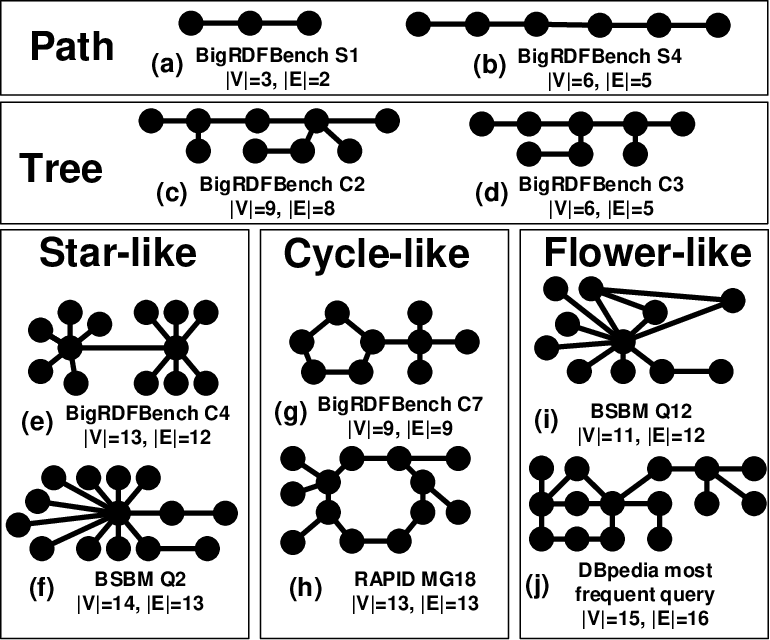
Ideally, real-world subgraph query logs can provide guidance to resolve this challenge. However, as remarked in Section 1, such data may be unavailable. Hence, we leverage results from a recent study (Bonifati2017) that analysed a large volume of real-world sparql query logs. It revealed that topologies of many real-world subgraph queries map to chains, trees, stars, cycles, petals, and flowers22 2 A petal is a graph consisting of a source node , target node and a set of at least 2 node-disjoint paths from to . A flower is a graph consisting of a node with three types of attachments: chains (stamens), trees that are not chains (the stems), and petals. A flower set is a graph in which every connected component is a flower. (Bonifati2017). Figure 3 depicts examples of these topologies in real-world subgraph queries extracted from BigRDFBench (saleem), BSBM (bsbm), Rapid (rapid), and DBPedia (dbpedia). Consequently, canned patterns in any gui should facilitate efficient construction of these topologies.
5.2. Topologies of Canned Patterns
We consider the following types of topological structures of canned patterns in order to facilitate construction of the above query substructures.
Path and cycle patterns. A subgraph query may contain paths of different lengths (i.e., chain) and/or cycles. Figure 3 depicts some examples. Hence, our canned patterns should expose representative -paths and -cycles in the underlying data. Given a graph , a -path, denoted as , is a walk of length containing a sequence of vertices where , such that all vertices in are distinct. A -cycle is simply a closed -path where .
Star and asterism patterns. Intuitively, a star is a connected subgraph containing a vertex where the remaining vertices are connected only to (i.e., neighbors of ). A -star is a single-level, rooted tree where , is the root vertex and is the set of leaves such that , , and . We refer to the root as the center vertex. Note that where is the minimum value of for which the single-level rooted tree is considered a star.
Real-world queries may contain multiple -stars that are combined together. For instance, the query topology in Figure 3(e) is a combination of 6-star and 7-star by merging on a pair of edges. Hence, our canned pattern topology also involves stars that form an asterism pattern by merging them on a pair of edges. Formally, given stars and merged edges where and , let be the center vertices such that . The asterism pattern of is defined as where , , )), , and .

-chord and composite chord patterns. Observe that tree-structured queries can be constructed by combining chains and stars (e.g., Figure 3(c)-(d)). However, they are insufficient to construct more complex petal and flower queries efficiently. In particular, petal and flower queries may often contain triangle-like structures. For example, the query in Figure 3(i) contains two triangles. Hence, at first glance it may seem that we can simply select different -trusses () of sizes within the plug specification as canned patterns. However, a subgraph query may not necessarily always contain -trusses. For instance, the query in Figure 3(j) contains multiple “triangle-like” structures as some common edges of triangles are missing. Consequently, the use of only -truss as a canned pattern may make query formulation inefficient as it demands deletion of multiple edges in order to construct a triangle-like query topology. This increases the number of steps required to formulate a query, thereby increase the formulation time. Hence, it is desirable to have “-truss-like” substructures as patterns.
| ID | Edge-at-a-time | Default patterns | Canned patterns |
|---|---|---|---|
| (c) | 17 | 6 [2 2-path + 1 square - 1 | 5 [4-path + 2 2-path + 2 merge] |
| edge + 1 edge + 1 merge] | 5 [4-star + 1 2-path + 1 node + 2 edge] | ||
| (e) | 25 | 11 [5 2-path + 1 node + 2 | 1 [A6,7] |
| edge + 3 merge] | 3 [5-star + 6-star + 1 edge] | ||
| (g) | 18 | 8 [4 2-path + 1 edge + 3 | 3 [5-cycle + 4-star + 1 merge] |
| merge] | 4 [6-path + 2-path + 1 edge + 1 merge] | ||
| (i) | 23 | 10 [square + 3 2-path + 1 | 5 [4-CP + 6-star + 1 node + 1 edge + 1 merge] |
| node + 2 edge + 3 merge] | 5 [CCPno(4,4) - 2 edge + 5-star + 1 merge] |
To this end, we extract two types of -truss-based structures as canned patterns, namely, k-chord patterns (-cp) and composite chord patterns (ccp). Intuitively, a -cp is a connected graph containing a truss edge (i.e., edge belonging to a -truss) and -2 triangles of . Formally, given a -truss for , the -chord pattern (-cp) associated with every edge where is defined as and where and . -cp can be considered as a building block of -trusses since it is found with respect to each edge in a given -truss. Examples of -cps (4-cp and 5-cp) are illustrated in Figure 4. We refer to the edge in a -chord pattern that is involved in (-2) triangles as a truss edge and the remaining edges as non-truss edges. For example, in Figure 4, edges and are truss edges whereas and are non-truss edges. Correspondingly, vertices of a truss edge (e.g., , , , ) are referred to as truss vertices. Observe that we can formulate a simple petal query in two steps by selecting the 4-cp pattern and deleting the truss edge.
To select larger canned patterns with greater structural diversity, we combine -cps to yield additional composite chord patterns (ccp) that occur in the underlying network. Observe that combining a set of -cps in different ways results in different patterns as demonstrated in Figure 4. However, this is an overkill as they are not only expensive to compute but also may generate patterns with higher density (higher cognitive load) or are larger than . Hence, we focus on the ccp generated by merging a single edge of two -cps as it not only reduces the complexity of ccp generation, but also produces ccps with lower density.
Unique small graph patterns. Lastly, we find small connected subgraphs that do not fall under above categories but occur multiple times in the underlying network.
Table 1 reports the number of steps taken by various modes of query construction of selected query topologies in Fig. 3. Observe that query construction using canned patterns often takes fewer number of steps compared to construction using only default patterns, emphasizing the need for patterns beyond the default ones. One can also formulate a specific query following multiple alternatives, i.e., using multiple sets of patterns (canned and default). This gives users the flexibility to formulate a query using these patterns in many ways, all of which often take fewer steps compared to the edge-at-a-time or default pattern-based modes.
6. Candidate Patterns Generation
In the preceding section, we classified the topologies of canned patterns broadly into “-truss-like” and “non--truss-like” structures. In this section, we describe how candidate canned patterns conforming to these topological categories are extracted from the underlying network .
We begin by providing an overview of the Tattoo algorithm. Algorithm 1 outlines the procedure. It first decomposes into truss-infested and truss-oblivious regions (Line 1) and then generates “-truss-like” and “non--truss-like” candidate patterns from these regions, respectively (Lines 2-8). Finally, it selects the canned pattern set from these candidate patterns based on the plug specification (Line 9). We discuss the decomposition of and candidate pattern generation in turn. In the next section, we shall elaborate on the selection of canned patterns from the candidate patterns.
| Data | Name | % () | % () | ||
|---|---|---|---|---|---|
| loc-Brightkite | 58K | 214K | 67.3 | 32.7 | |
| loc-Gowalla | 197K | 950K | 78.2 | 21.8 | |
| com-DBLP | 317K | 1.05M | 93 | 7 | |
| com-Amazon | 335K | 926K | 77.2 | 22.8 | |
| RoadNet-PA | 1.09M | 1.54M | 12.7 | 87.3 | |
| com-Youtube | 1.13M | 2.99M | 46.8 | 53.2 | |
| RoadNet-TX | 1.38M | 1.92M | 12.5 | 87.5 | |
| as-Skitter | 1.7M | 11M | 79.1 | 20.9 | |
| RoadNet-CA | 1.97M | 2.77M | 12.6 | 87.4 | |
| com-LiveJournal | 4M | 34.7M | 83.2 | 16.8 |
6.1. Truss-based Graph Decomposition
In order to extract “non--truss-like” and “-truss-like” structures as candidate patterns, we first decompose a network into sparse (containing non-trusses) and dense (containing trusses) regions. The latter region is referred to as truss-infested region (tir graph) and the former truss-oblivious region (tor graph), and are denoted by and , respectively. Table 2 reports the sizes of and in several real-world networks measured as the percentage of the total number of edges. We observe basically consists of relatively large connected subgraphs that comprise multiple -trusses. On the other hand, mainly consists of chains (i.e., paths), stars, cycles, and small connected components. Furthermore, although some networks have small (e.g., com-DBLP), there are networks where is large (e.g., RoadNet-CA), encompassing up to of the total number of edges. Consequently, by decomposing a network into and , we can improve efficiency by limiting the search for -truss-like patterns in instead of the entire network and extract non-truss-like patterns from . Additionally, generating candidate patterns of aforementioned topological categories from both tir and tor graphs enables us to select a holistic collection of patterns having higher coverage and diversity. Cognitive load of the pattern set is often reduced when patterns from both regions are considered due to the sparse structure of tor.
Tattoo utilizes the state-of-the-art truss decomposition approach in (wang2012) to decompose into and . Briefly, this approach identifies -trusses () in iteratively by removing edges with support less than from . Hence, our graph decomposition algorithm adapts it to assign 2-truss as and the remaining -trusses as .
We keep track of the edge trussness (denoted as ) in . Since the goal is to select canned patterns with maximum size , the upper bound of edge trussness is set to this value. The algorithm first identifies the support of each edge. Then, regions of the data graph are iteratively extracted by removing edges with the lowest support, starting from the sparsest (i.e., ) to the densest. In particular, Tattoo considers all edges with as sparse regions and these edges form the tor graph . The remaining edges form the tir graph .
In summary, the above approach makes the following two simple modifications to the truss decomposition technique in (wang2012): (1) instead of storing each -truss as a separate graph, it stores 2-truss as and the remaining -trusses are combined as a single graph ; (2) it assigns a trussness value to every edge in and . The worst-case time and space complexities of this algorithm are and , respectively (wang2012).
6.2. Patterns from a TIR Graph
Next, we generate -cps and ccps as candidate patterns from a tir graph. For each pattern we also compute its frequency as it will be used subsequently to measure its coverage. We discuss them in turn.
Generation of -chord patterns. Algorithm 2 describes generation of the -cps. In particular, we can find -cps with respect to each edge in a given -truss. For instance, every edge in a 4-truss and a 5-truss is part of at least 2 and 3 triangles, respectively. Observe that the -chord pattern of an edge is simply the edge itself. Hence, Tattoo generates -cps for . The frequency of a -cp is measured by the frequency of the pattern occurring in , which is essentially the number of edges having trussness greater than or equals to (Lines 13 to 20). Formally, given a tir graph and a -chord pattern , the frequency of is defined as . Then, the set of -cps of a is simply the set of patterns whose frequency is greater than 0. We first generate -chord patterns in and then compute their frequencies using edge trussness.

Lemma 6.1.
The worst-case time and space complexities of -cp generation are and , respectively.
Generation of composite chord patterns. Next, we generate the ccps. Specifically, we generate the following categories of ccps based on different ways of merging truss and non-truss edges.
Definition 6.2.
Let and be two -chord patterns where and are truss vertices. Then, we can generate the following categories of composite chord patterns of and by merging and as follows:
- (1)
: merge the truss edge of with a non-truss edge of .
- (2)
: merge the truss edge of with a non-truss edge of .
- (3)
: merge a non-truss edge of with a non-truss edge of such that there is an overlapping truss vertex.
- (4)
: merge a non-truss edge of with a non-truss edge of such that there is no overlapping truss vertex.
Figure 4 depicts examples of these four categories of ccps. When the context is clear, we shall simply refer to a ccp as . A keen reader may observe that it is possible to create another ccp by merging the truss edge of with the truss edge of . However, this ccp is in fact a -cp where . For instance, when and in Figure 4 are merged on their truss edges, the resultant pattern is a -cp. Also, combining two -cps always yields a -cp (Lemma 6.3). Since -cps have already been handled earlier, these combinations are ignored.
Lemma 6.3.
Two -cps always yield a ccp that is -cp.
We now elaborate on how the ccps and their frequencies are computed in Tattoo efficiently. We shall introduce two terminologies related to node and edge neighbourhoods of a ccp to facilitate exposition. Given an edge in a -truss, the -ccp node neighbourhood (denoted as ) of is a set of vertices adjacent to and such that , and where . The -ccp edge neighbourhood (denoted as ) of is the set of edges adjacent to such that , where . Figure 5 illustrates examples of -ccp node and edge neighborhoods. For instance, consists of since and .
Lemma 6.4.
Given a truss edge , there is at least a -chord pattern on if .
Frequencies of and . Consider two different -cps. and involve merger of a truss edge belonging to one -cp with a non-truss edge belonging to another -cp. Given two -cps and , let edges and be the truss edges of and , respectively. Intuitively, a pattern is a if it contains an embedding of and of whereby there is an edge in the pattern that belongs to the two embeddings such that is a truss edge of ’s embedding and is a non-truss edge of ’s embedding, respectively. In other words, and can form a ccp () by merging a truss edge from with a non-truss edge from if the following conditions are satisfied: (a) Condition 1: There is a pattern on containing . (b) Condition 2: There is a pattern on where .
Note that due to Lemma 6.4, Condition 1 holds if where . Further, if , then the pattern must exist. Hence, Tattoo checks the conditions iteratively on decreasing and skips checks for if the conditions are satisfied for . The frequency of is simply the number of such edges. For , the approach is the same by swapping with .

Frequencies of and . Recall that (Def. 6.2) a single-edge merge can also involve the merger of two non-truss edges, each from a different -cp. Each non-truss edge contains a truss vertex. There are two ways in which two non-truss edges can merge as shown in Figures 6(b) and (c). In the former (resp. latter), vertex pairs () (resp. ()) and () (resp. ()) are merged. Hence, a pattern is a if it contains at least one embedding of a structure shown in Figure 6(b) which we refer to as the skeleton structure of (denoted as ). Hence, we can search for the of a in a tir graph to compute its occurrence and frequency. Specifically, a can be obtained if the followings are satisfied: (a) Condition 1: There is a pattern on its truss edge which contains . (b) Condition 2: There is a pattern on its truss edge which contains .
Note that Condition 1 holds if (Lemma 6.4). Similarly, Condition 2 holds if . Further, if , then the pattern must exist. The frequency of a is simply the number of skeleton structures in a tir graph.
is very similar to except that the truss vertices of the merged edges are not combined during the merger. Figure 6(c) illustrates the skeleton structure of a (), which occurs in all . The frequency of a is the number of skeleton structures .
Observe that since and can be swapped. The same is true for and . Hence, when combining two -cps, we only consider the case when .
Algorithm. Putting the above strategies together (outlined in Algorithm 3), the ccps are computed as follows. For each edge in , compute the -ccp node and edge neighbourhoods (Lines 4-5). Next, it computes the four types of ccps (Lines 6-13) based on the aforementioned strategies. Note that the smallest ccp generated is a ccp(3,4) due to Lemma 6.3. Also, we only compute instead of both and as is covered when and are swapped.
Theorem 6.5.
The worst-case time and space complexities of the ccp generation technique are and , respectively.
6.3. Patterns from a TOR Graph
Generation of candidates from a tor graph consists of two phases: star pattern extraction and small pattern extraction. The former extracts star and asterism patterns. Subsequently, the edges involved in these patterns are removed from resulting in further decomposition of the tor graph. The resultant graph is referred to as the remainder graph (). Then, the second phase extracts paths, cycles, and small connected subgraphs from .
Extraction of star and asterism patterns. The frequencies of these patterns can be derived directly from their definitions (Sec. 5.2). Specifically, and where , , and . Algorithm 4 outlines the procedure. The star and asterism patterns are extracted in Lines 2 to 22 and Lines 6 to 20, respectively. Briefly, asterism patterns are found using breadth-first search (bfs). A vector of vertices is used to keep track of star centers in an asterism pattern. We “grow” the pattern by adding a neighbouring vertex of the current star center being considered only if and when the size of the grown pattern is less than or equals to .
Lemma 6.6.
The worst-case time and space complexities of star and asterism pattern extraction are and , respectively.
Extraction of small patterns. The remainder graph is primarily composed of small connected components such as paths, cycles, and subgraphs with unique topology. Algorithm 5 outlines the extraction of these small patterns and we denote -cycle as and subgraphs with unique topology as . Given a graph , a -path, denoted as , is a walk of length containing a sequence of vertices where , such that all vertices in are distinct. A -cycle is simply a closed -path where . We refer to small subgraph patterns as connected components in that are neither -paths nor -cycles. Note that 1-path, 2-path, 3-cycle and 4-cycle are basic building blocks of real-world networks (milo2002). Recall that in Tattoo, we consider them as default patterns and they are not part of the candidate canned pattern set. Hence, we extract all -paths for (Lines 19-21) and -cycles for (Lines 22-24) and their frequencies. After that, small connected subgraphs and their corresponding frequencies are extracted.
Lemma 6.7.
Worst-case time and space complexities to find small patterns are and , respectively.
Remark. Exponential time complexity of the small pattern extraction phase is due to the isomorphism check. The time cost is small in practice due to the small size of candidate patterns and their number is typically small in .
7. Selection of Canned Patterns
In this section, we describe the algorithm to select canned pattern set from the generated candidate patterns. We begin by presenting the theoretical underpinning that influences the design of our algorithm.
7.1. Theoretical Analysis
Due to the hardness of the cps problem, we design an approximation algorithm to address it. We draw on insights from a related problem, team formation problem (tfp) (chen2004; bhowmik2014), which aims to hire a team of individuals from a group of experts for a specific project where . Bhowmik et al. (bhowmik2014) proposed that several aspects should be considered in tfp, namely, skill coverage (skill), social compatibility (social), teaming cost (team) and miscellaneous aspects such as redundant skills avoidance (red) and inclusion of selected experts (exp). The formulation of tfp is given as were , , , and are non-negative coefficients that represent the relative importance of each aspect of team formation (bhowmik2014). The goal is to find a team where the non-negative and non-monotone function is maximized. According to (bhowmik2014), this formulation can be posed as an unconstrained submodular function maximization problem which is NP-hard for arbitrary submodular functions.
Selecting a set of canned patterns in cps is akin to hiring a team of individuals in tfp where , , correspond to , and , respectively. Hence, cps can be formulated in the form (Definition 7.1) where is the set of candidate patterns which yields an optimized .
Definition 7.1.
[Pattern Set Score] Given a pattern set , the score of is where , and are the coverage, similarity and cognitive load of , respectively.
Definition 7.2.
[Good Candidate Pattern] Given a pattern set and two candidate patterns and , is considered a good candidate pattern if and is added to instead of .
Note that Definition 7.2 can be utilized for determining inclusion of a candidate pattern in . Next, we analyze the properties of , , , and the pattern score.
Lemma 7.3.
Coverage of a pattern set , , is submodular.
Lemma 7.4.
The similarity (resp. cognitive load) of a pattern set , (resp. ), is supermodular.
Theorem 7.5.
The pattern set score in Definition 7.1 is a non-negative and non-monotone submodular function.
Similar to in tfp, in cps is non-negative and non-monotone. However, unlike tfp, cps imposes a cardinality constraint where is at most . Thus, cps can be posed instead as a maximization of submodular function problem subject to cardinality constraint (buchbinder2014).
7.2. Coverage, Cognitive Load, and Similarity
Next, we quantify the coverage, cognitive load, and similarity measures used in the pattern score .
Coverage. Recall from Section 4, we can compute the coverage of a pattern as . Since the edge sets of and are mutually exclusive, we further modify to include a weight factor to account for effects exerted by the sizes of and . Specifically, where for patterns obtained from . However, exact computation of coverage for each candidate pattern is prohibitively expensive. Hence, we approximate as follows: . Observe that is in fact the upper bound of when no isomorphic instances of in overlap. Any superior upper bound that can be computed efficiently can be incorporated. Unlike , computation of requires only , which is significantly more efficient.
The order of pattern extraction in (e.g., extracting stars and asterisms before small patterns) may affect the frequency of the extracted patterns. Hence, normalization of is performed for each class of patterns (-cp, ccp, star, asterism, and small pattern) as follows:
| (2) |
where represents a class of pattern. Specifically, we compute -cps and ccps in . Stars, asterisms and small patterns are computed in . The normalized is in [0-1].
Cognitive Load. (catapult; midas) measure cognitive load based on size and density only, ignoring edge crossings. Since it is designed for a collection of small- or medium-sized data graphs, it is a reasonable measure as in many applications such data graphs have very few edge crossings (e.g., chemical compounds), if any. In contrast, edge crossings occur frequently in large networks and hence cannot be ignored in our context. In fact, Huang and colleagues examined the effect of edge crossings on mental load of users and found that cognitive load displays a relationship with edge crossings that resembles the logistic curve (huang2010) where is the curve’s maximum value, is the value of sigmoid’s midpoint and is the logistic growth rate (zeide1993).
Lemma 7.6.
The crossing number (i.e., number of edge crossings) of any simple graph with at least 3 vertices satisfies .
Hence cognitive load of a pattern is computed based on the size (), density () and edge crossing (). if is planar. Otherwise, it is . We modelled the normalized cognitive load function in Tattoo according to the logistic curve:
| (3) |
Parameters of are set empirically to ensure even distribution within the range of [0 1].
Similarity. Given a partial pattern set and two candidate patterns and , Tattoo selects preferentially to add to if . To this end, we utilize NetSimile, a size-independent graph similarity approach based on distance between feature vectors (berlingerio2013). It is scalable with runtime complexity linear to the number of edges.
7.3. CPS-Randomized Greedy Algorithm
The canned pattern selection algorithm is as follows. First, it retrieves the default pattern set (-path, -path, -cycle and -cycle). Next, it prunes candidate patterns whose sizes do not satisfy the plug specification or are “nearly-unique” (i.e., where is a pre-defined threshold). Note that the latter patterns have very low occurrences in and are unlikely to be as useful for query construction in their entirety33 3 In the case, a user is interested in patterns with low coverage, can be set to 0 along with the reduction in in (Defn. 7.1).. Then, it selects from the remaining candidates.
Recall from Section 7.1, the cps problem can be cast as a maximization of submodular function problem subject to cardinality constraint. Recently, the algorithm community has proposed a technique with quality guarantee in (buchbinder2014) to address it. We exploit this approach, referred to as CPS-Randomized Greedy (CPS-R-Greedy, Algorithm 6), in our cps problem. To the best of our knowledge, this approach has not been utilized for graph querying.
In particular, CPS-R-Greedy extends the discrete greedy algorithm (nemhauser1978) using a randomized approach. At every step, a random candidate pattern is chosen from a set of “reasonably good” candidates (Lines 19-22). Intuitively, these candidates should have very few edge crossings, good coverage and are different from patterns already in . These candidates are identified as follows. For every candidate pattern , we compute the pattern set score (Definition 7.1) assuming is added to the canned pattern set. A “good” candidate improves on the score of the set when it is added (Definition 7.2). Note that , , and changes as changes. Hence, we recompute them at every iteration. Then, we randomly select a “good” candidate and assign it to . The algorithm terminates either when the set contains the desired number of patterns or when there exists no more good candidates. The following quality guarantee can be derived from (buchbinder2014).
Theorem 7.7.
CPS-R-Greedy achieves -approximation of cps.
Theorem 7.8.
CPS-R-Greedy has worst-case time and space complexity of and , respectively, where and are the number of vertices and edges in the largest candidate pattern.

Example 7.9.
Consider a gui and a plug . Suppose there are four default patterns and five candidate patterns (i.e., ) as depicted in Figure 7. Let . The algorithm first removes since . Then, for the remaining patterns in , each is considered in turn to be added to by exploiting CPS-R-Greedy technique. It first considers adding to and computes the resulting coverage (), cognitive load () and similarity (). The pattern set score of is then computed using Defn. 7.1. The scores of the other candidate patterns are computed similarly. Suppose the scores are 0.72, 0.63, 0.54, 0.68 for , , , , respectively. Then, in the first iteration, is selected (and removed from subsequent iterations) and the current best score is updated to 0.72. In the next (i.e., final) iteration, the candidates are again considered in turn to be added to and corresponding pattern set scores are computed. However, unlike the first iteration, only those candidates whose scores are greater than are considered. Let the scores of , and be 0.81, 0.7 and 0.77, respectively. Then, a candidate will be randomly selected from or . Suppose is chosen, then the final pattern set is .
8. Performance Study
Tattoo is implemented in C++ with GCC 4.2.1 compiler. We now report the key performance results of Tattoo. All experiments are performed on a 64-bit Windows 10 desktop with Intel(R) Core(TM) i7-4770K CPU (3.50GHz) and 16GB RAM.
8.1. Experimental Setup
Datasets. We evaluate Tattoo’s performance using 10 large networks (Table 2) from snap (http://snap.stanford.edu/data/index.html) containing up to 34.7 million edges.
Algorithms. State-of-the-art guis for large networks (PH+17; PH+18) do not support canned patterns. Hence, we compare Tattoo with the following baselines: (a) Catapult (catapult): We assign same labels to all nodes of a network and partition it into a collection of small- or medium-sized data graphs using Metis (karypis1997). Then the algorithm in (catapult) is used to select canned patterns. (b) Use graphlets, frequent subgraphs, random patterns, default patterns, and edge-at-a-time (i.e., pattern oblivious): -node graphlets where are generated using the approach in (chen2016). Random patterns are generated by randomly selecting subgraphs of specific sizes from a network. The number of candidates per size follows a uniform distribution. Frequent subgraphs are generated using Peregrine(jamshidi2020) (downloaded from (peregrine-c)). These subgraphs are considered as candidates from which the canned patterns are selected using our algorithm in Section 7.3.
Query sets and GUI. We use different query sets for the user study and automated performance study. We shall elaborate on them in respective sections. The gui used for user study is viewable at https://youtu.be/sL0yHV1eEPw.
Parameter settings. Unless specified otherwise, we set , , , , and .
Performance measures. We measure the performance of Tattoo using the followings: (1) Run time: Execution time of Tattoo. (2) Memory requirement (mr): Peak memory usage when executing Tattoo. (3) Reduction ratio (denoted as ): Given a subgraph query , where is the minimum number of steps required to construct when is used and is the total number of steps needed when edge-at-a-time approach is used. Note that the number of steps excludes vertex label assignments which is a constant for a given regardless of the approach. For simplicity in automated performance study, we follow the same assumptions in (catapult): (1) a canned pattern can be used in iff ; (2) when multiple patterns are used to construct , their corresponding isomorphic subgraphs in do not overlap. In the user study, we shall jettison these assumptions by allowing users to modify the canned patterns and no restrictions are imposed (i.e., does not need to be minimum). Smaller values of imply better pattern diversity. For ease of comparison, the diversity plots are based on the inverse of .
8.2. User Study
We undertake a user study to demonstrate the benefits of using our framework from a user’s perspective. 27 unpaid volunteers (ages from 20 to 35), who were students of, or, researchers within different majors took part in the user study. None of them has used our gui prior to the study. First, we presented a 10-min scripted tutorial of our gui describing how to visually formulate queries. Then, we allowed the subjects to play with the tool for 15 min.
For each dataset, 5 subgraph queries with size in the range [10-28] are selected. These queries mimic topology of real-world queries containing various structures described in Section 5.2. To describe the queries to the participants, we provided printed visual subgraph queries. A subject then draws the given query using a mouse in our gui. The users are asked to make maximum use of the patterns to this end. Each query was formulated 5 times by different participants. We ensure the same query set is constructed in a random order (the order of the query and the approach are randomized) to counterbalance learning effects.


The canned patterns on the gui are grouped by size and displayed using ForceAtlas2 layout (jacomy2014) in different pages according to their sizes. This multi-page-based organization yields faster average query formulation time and fewer steps compared to other alternatives.
Display layout of canned patterns. We first explore 3 different graph layout algorithms, namely, ForceAtlas2 (jacomy2014), Fruchterman Reingold (fr) (fruchterman1991) and Dagre (pettitt2014) to determine the most suitable layout for displaying canned patterns our gui. Ten participants were asked to construct a set of 5 queries each for the Amazon and YouTube datasets. Each participant repeated this experiment 3 times where a different graph layout was used on the canned pattern set each time. Figures 8 and 9 plot the average query formulation time and average number of steps. In general, the ForceAtlas2 layout yielded faster average qft compared to fr and Dagre. Participants also took fewer steps using ForceAtlas2 compared to the rest. Hence, in subsequent experiments, Tattoo leverages ForceAtlas2 layout to display the canned patterns.


Learning effect. Since the same query set is used repeatedly for each approach, there may be a learning effect where volunteers start to commit the query set to memory if the study is conducted in a fixed order. Particularly, approaches that are tested latter in the study may gain an unfair advantage over earlier approaches. We investigate it further with an experiment. Ten participants () were asked to construct 5 queries on the Amazon and YouTube datasets in a fixed order while another ten participants ( where ) were asked to construct the same query set in a random order (the order of the query and the approach are randomized) to minimize learning effects. Figure 10 reports the average time taken for query formulation. Interestingly, formulation time is generally faster using Tattoo’s canned patterns compared to graphlets regardless of the order on the query and approach. We further examined the difference in average formulation time (i.e., ) across queries and datasets for these two orders. In particular, the average time difference for Amazon (resp. YouTube) is 5.5s (resp. 5.5s) and 5.9s (resp. 3.7s) for fixed order and random order, respectively. This is possibly due to the learning effect. Hence, in subsequent experiments we follow the randomized order to minimize learning effect.
Visual mapping time. In order to use canned patterns for query formulation, a user needs to browse the pattern set and visually map them to her query. We refer to this as visual mapping time (vmt). For each pattern used, we record the pattern mapping time (pmt) as the duration when the mouse cursor is in the Pattern Panel to the time a user selects and drags it to the Query Canvas. The vmt of a query is its average pmt. Intuitively, a longer vmt implies greater cognitive load on a user. Figure 11 shows the vmt of tattoo patterns, graphlets, frequent subgraphs, and random patterns on am and yt datasets. On average, Tattoo patterns consume the least vmt.
We investigate the effect of various gui canned pattern layout options (i.e., single page (); group by size (); 4 per page (); 8 per page (); 16 per page (); sort by cognitive load (), diversity () and sort by coverage ()) on vmt for AM and YT datasets. Note that arranges the patterns in the order that they are identified. The plug was set to . Figure 12 shows that the average vmt for layout options with multiple pages tends to be shorter (up to 33.1%) than those in a single page (i.e., , , and ). When the patterns are organized in pages, an increased number of pages reduces the need for a user to scroll and browse the patterns on a particular page and increases the need to toggle between various pages to identify useful patterns. Compared to single page options, the multi-page options (, , , ) achieve superior performance primarily due to the former. Hence, the multi-page-based organization is used for our user study.



Query formulation time (qft) and number of steps. Figures 13 and 14 plot the average qft and the average number of steps taken, respectively, for am and yt. Note that a qft includes the vmt and the steps include addition/deletion of nodes and edges and merger of nodes. As expected, the edge-at-a-time approach took the most steps. Paired t-test shows that the superior performance of Tattoo is statistically significant () for 79.4% of the comparisons (Figure 15). In particular, it takes up to 18X, 9.3X, 6.7X, 8X, 9X, and 9X fewer steps compared to edge-at-a-time, default pattern, random patterns, graphlet, frequent patterns, and Catapult-generated patterns, respectively. For qft, Tattoo is up to 9.7X, 8.6X, 9X, 6.6X, 7.1X, and 7.4X faster, respectively. The results are qualitatively similar in other datasets. Note that we can run Catapult only on am for reasons discussed later.
Effect of . The number of patterns on a gui may also impact a user cognitively as larger means a user needs to browse more patterns to select relevant ones. Hence, we investigate the effect of on qft and the number of steps (Figure 16). Interestingly, qft and steps are reduced by average of 12% and 22% (maximum reduction of 77% and 80%), respectively, when is increased from 5 to 30. Increase in exposes more patterns that could be leveraged for query formulation, reducing query formulation steps. Further, it results in two opposing effects: (1) longer time needed to browse and select appropriate patterns (longer vmt) and (2) potentially more and larger patterns available for query construction resulting in fewer construction steps and shorter qft. The latter effect dominates.


Qualitative evaluation. We also conducted a post-study questionnaire to gain some qualitative feedback on Tattoo. Overall, all participants prefer to use pattern-at-a-time approach compared to edge-at-a-time approach and Tattoo’s canned patterns are rated the most useful with average rating of 4.5 on a 5-point Likert scale. Graphlets, frequent and random patterns have average ratings of 3.5, 4 and 1.75, respectively.
In addition, participants were queried using an adapted nasa-tlx (hart1988) questionnaire (on a 5-point Likert scale) regarding the mental demand, performance and frustration level of query formulation using canned patterns generated from various approaches. Briefly, nasa-tlx is a commonly used tool for assessing perceived workload based on user inputs in the form of a questionnaire and consists of ratings for 6 categories44 4 Mental demand can be interpreted as the cognitive load on the user; Physical demand assesses the amount of physical activity required for the task; Temporal demand is related to the time pressure experienced based on the pace of the task; Performance measures a user’s satisfaction with performance of the task; Effort can be interpreted as the overall mental and physical demand needed to perform the task; Frustration level sets out to measure user’s feelings (i.e., irritated, stressed and annoyed versus content, relaxed and complacent) during performance of the task., namely, mental demand, physical demand, temporal demand, performance, effort and frustration. Since we do not impose a time limit on the query formulation task, there is no temporal demand. Physical demand is also negligible in our problem setting. In particular, effort and mental demand are equivalent in this case and can be associated directly with cognitive load. The mental demand is 2.5, 3, 3.5 and 4.25 for Tattoo, frequent patterns, graphlets and random patterns, respectively, where larger values imply greater mental demand. In terms of performance, it is 4.25, 4, 4 and 3.75, respectively, where larger values are associated with better performance. The frustration level is 2.75, 2.75, 3 and 4, respectively, where larger values relates to more frustration. This highlights the benefits of canned patterns generated by Tattoo.
Some users elaborated on their preferences. Table 3 lists the key comments by these users. Several users highlighted that they found edge-at-a-time approach tedious to use compared to pattern-at-a-time approach due to the repetitive task of drawing vertices and edges. This is consistent with hci research as remarked in Section 1. They also felt that canned patterns of Tattoo are more diverse and easy to map to the query graphs. Hence, using them during query construction do not require much effort, and the patterns are useful in speeding up query formulation. Lastly, several users highlighted the usefulness of default patterns in extending other larger canned patterns during query formulation.
| Index | Comment |
|---|---|
| 1 | I like to use canned patterns to draw a query graph because it is faster and less tedious. Constructing the query graph each vertex and each edge at a time is just too tedious and boring! |
| 2 | The random and graphlet patterns appear very cluttered and confusing!. It takes me considerable time to figure out if I can use them or not for my query. |
| 3 | The default patterns are simple and easy for me to figure out. But I need to choose several of them repeatedly for a large query. The Tattoo patterns are a great complement to the default patterns to make the drawing faster. |
| 4 | Tattoo patterns are more varied and I can usually find some patterns to use for drawing subgraph queries. |
| 5 | I find it easy to map the Tattoo patterns to a query compared to other patterns like the random ones. It is actually much faster to construct a query using them than if I were to draw the vertices and edges one at a time. |
| 6 | I like the ease of use of the gui. I can just use one interface to query different datasets. I don’t need to switch to different interfaces for different sources. |
| 7 | The default patterns are very useful for extending other bigger patterns like those from Tattoo and graphlets when I draw a subgraph query. |
8.3. Automated Performance Study
In this section, we evaluate Tattoo from the following perspectives. First, we compare the runtime and quality of patterns of Tattoo with the baseline approaches (Exp 1, 2). Second, we present results that support our design decisions (Exp 3, 4, 5). To this end, we generate 1000 queries (size [4-30]) for each dataset where 500 are randomly generated and remaining (evenly distributed) are path-like, tree, star-like, cycle-like and flower-like queries.
Exp 1: Run time. First, we evaluate the generation time of different patterns types in canned pattern sets. Figure 17 (top) shows the results. In particular, generation of chord-like patterns requires significantly more time (up to 146% more for lj) than other pattern types. This is primarily due to checks for different types of edge merger required for ccps. Figure 17 (bottom) reports the time taken by various phases of Tattoo as well as runtime of Catapult. Tattoo selects canned patterns efficiently within a few minutes. Observe that the time cost for the small pattern extraction phase is small in practice. In general, pattern selection is the most expensive phase and requires a couple of minutes or less. Results are qualitatively similar for other datasets. Figure 18 plots the memory requirement for Tattoo. It is largely dependent on the size of the dataset where the largest dataset has the greatest memory cost.
Lastly, observe that Tattoo is 735X faster than Catapult, which is not designed for large networks. Except am, other datasets either cannot be processed by Metis or fail to generate patterns in a reasonable time (within 12 hrs) due to too many possible matches of unlabelled graphs that require expensive graph edit distance computation. In the sequel, we shall omit discussions on Catapult.
Exp 2: Comparison with graphlets, frequent subgraphs, and random patterns. Next, we compare Tattoo’s patterns with those of graphlets (30 patterns derived from graphlets). Figure 19 reports the results. Observe that Tattoo’s patterns are superior to graphlets in all aspects. The results are qualitatively similar for other datasets. Note that coverage is not examined since it is 100% in all cases as all queries can be constructed using 2-node graphlet.
We compare the canned pattern set derived from frequent subgraphs generated by Peregrine (denoted as ) to those generated by Tattoo. We observe that Peregrine failed to extract larger size patterns (i.e., ) within 12 hrs for all networks. Specifically, for rp, rc, and rt (resp. am), it was able to extract frequent patterns of size (resp. ) within 2.5 hrs. For bk and db (resp. yt, lj, sk, and go) it can extract upto size (resp. ) within 2.5hrs. However, it took around 39 hrs on am to yield a meaningful number of candidate patterns (994 patterns with size and ) when the minimum threshold is set to 100. Hence, Tattoo is orders of magnitude faster than frequent pattern-based solution. Consequently, we restrict the canned pattern sets of both Tattoo and to 30 patterns with and for am in our experiments for fair comparison. Consistent with our user study, Tattoo’s pattern set is superior to in most aspects. The average coverage, cognitive load, diversity and for Tattoo (resp. Peregrine) are 0.3 (resp. 0.27), 0.15 (resp. 0.14), 0.64 (resp. 0.59) and 0.23 (resp. 0.24), respectively.
The comparison with random patterns are reported in Figure 20. We observe that Tattoo’s patterns result in higher , and are significantly lower in cognitive load (up to 3.2X) when compared to random patterns. Tattoo’s patterns is up to less diverse compared to random patterns. The greater diversity of the random pattern set is likely due to the unrestricted way in generating the random patterns as compared to pattern generation of Tattoo which are partially derived from defined structures such as trusses, paths, cycles and stars. Despite the greater diversity, random patterns are more difficult to use in practice (Section 8.2) likely due to the greater cognitive load necessary to interpret the patterns.


Exp 3: Measuring cognitive load. We now justify the choice of our proposed cognitive load measure. Specifically, we compare several ways of measuring cognitive load of a pattern , namely, ; ; ; (used in (catapult)); and (recall , , from Sec. 7.2). 20 volunteers were asked to rank the visual representations of six graphs (Figure 21) of varying sizes and topology, in terms of cognitive effort required to interpret these graphs. A “ground truth” ranking for these graphs is obtained based on the average ranks assigned by the volunteers. Then, the graphs are ranked according to the five cognitive load measures and compared against the ground truth using Kendall’s (kendall1948). and achieve the highest . We select as the cognitive load measure since it is in the range of and facilitates easy formulation of a non-negative and non-monotone submodular pattern score function (Theorem 7.5).
Exp 4: Chord patterns vs -trusses. Next, we show the benefits of using -cp/ccps (i.e., -truss-like structures) compared to simply utilizing -trusses as topology for canned patterns (recall from Section 5.2). We generate 100 random queries of size [4-30] from and these yielded 11 -cp/ccps and 3 -trusses. Observe that -cp/ccps improve both and diversity but have poorer cognitive load (Figure 22). Here the cognitive load and diversity of a pattern set is the average value for respective measures. Importantly, more -cp/ccps than -trusses satisfying the plug are generated due to relaxed structure of the former. For instance, the rp dataset produces more -cp/ccps due to the small size of (see Table 2). That is, -trusses may not result in sufficient number of canned patterns on a gui. Hence, chord patterns improve the quality of canned patterns in terms of and diversity compared to -trusses and yielded more candidate patterns.

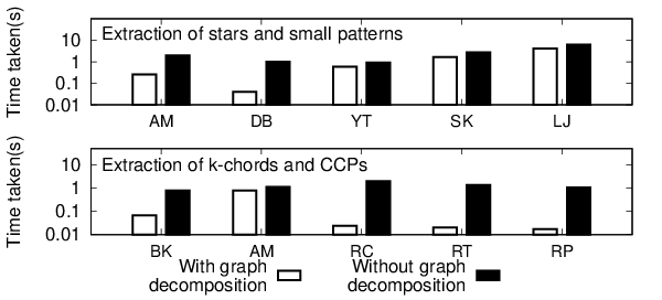
Exp 5: Generating patterns from and . Lastly, we examine the (a) benefits brought by graph decomposition on pattern extraction and (b) the characteristics (i.e., average cognitive load, , and average diversity) of canned pattern sets generated from and and compare them with the default patterns (i.e., - and -oblivious). Graph decomposition reduces the pattern extraction time for -truss-like structures, as well as, stars and small patterns across all datasets (Figure 23). The effect is most prominent for extraction of -truss-like structures where it is up to 81.5X faster when graph decomposition is applied. For extraction of stars and small patterns, it is up to 24.3X faster with graph decomposition. Hence, this justifies our decision to perform truss-based graph decomposition.
Figure 24 reports the characteristics of the canned pattern sets. Note that coverage is 100% for the three cases as all queries can be constructed using the default pattern (Figure 7). On the other hand, Tattoo’s canned patterns achieve and average coverage of and , respectively. Observe that patterns obtained from and contribute to higher and greater diversity over the default patterns, respectively. That is, despite 100% coverage of the latter, it is less efficient (i.e., more number of steps for query formulation) than the former. Also notice the increase in cognitive load due to the inclusion of chord-like patterns as they are likely to be denser than others. Hence, patterns from and complement the default patterns by improving and diversity.

9. Case Study
In this section, we describe the application of Tattoo for visual query formulation on the Amazon and RoadNet-TX datasets. We generate 30 canned patterns of sizes between 4 and 15 from each of these datasets. Figures 25(a) and 25(b) depict some of the patterns selected from Amazon and RoadNet-TX, respectively. Observe that the patterns are different for different datasets. Specifically, patterns in red rectangle boxes in Figures 25(a) are not found in Figures 25(b) and vice versa. This emphasizes the fact that different datasets may expose different collection of canned patterns to aid efficient query formulation. Second, observe that the patterns have low cognitive load as one can easily recognize their topology with a quick glance. In particular, patterns encapsulated by blue ellipses (solid lines) in Figures 25(a) and (b) are examples of some patterns derived from .
We now illustrate efficient query construction using canned patterns. Suppose one is interested in making a new movie involving Ben Affleck and Matt Damon. She would like to identify other actors that have prior working experience with these two actors. She may construct a subgraph query such as the one in Figure 25(c) to query the Amazon dataset containing movie titles and associated actors. Query formulation takes 8 steps () by utilizing one canned pattern (highlighted by green ellipse with broken line in Figure 25(a)) and adding an edge. Note that the steps taken include vertex label assignment. In comparison, edge-at-a-time requires a total of 20 steps ().
10. Conclusions & Future Work
Canned patterns play a pivotal role in supporting efficient visual subgraph query formulation using direct-manipulation interfaces. We present Tattoo, which takes a data-driven approach to selecting them from the underlying network by exploiting real-world query characteristics and optimizing coverage, diversity, and cognitive load of the patterns. Our experimental study demonstrates superiority of our framework to several baselines. As part of future work, we plan to explore the problem in a distributed settings.
Acknowledgements. The first four authors are supported by the AcRF Tier-2 Grant MOE2015-T2-1-040. Wook-Shin Han was supported by Institute of Information & communications Technology Planning & Evaluation (IITP) grant funded by the Korea government (MSIT) (No. 2018-0-01398). Byron Choi is supported by HKBU12201518.
References
- [1] 2021. Neo4j Bloom. https://neo4j.com/bloom.
- [2] 2021. BSBM. http://wifo5-03.informatik.uni-mannheim.de/bizer/berlinsparqlbenchmark/spec/20080912/index.html#queriesTriple.
- [3] 2021. Peregrine.https://github.com/pdclab/peregrine.
- [4] 2021. RAPID. https://research.csc.ncsu.edu/coul/RAPID/RAPIDAnalytics/.
- [5] 2021. Stanford Large Network Dataset Collection. http://snap.stanford.edu/data/index.html.
- [6] Foto N. Afrati, Dimitris Fotakis and Jeffrey D. Ullman. 2013. Enumerating subgraph instances using map-reduce. In IEEE 29th International Conference on Data Engineering. IEEE, 62-73.
- [7] Nesreen K. Ahmed, Jennifer Neville, Ryan A. Rossi and Nick Duffield. 2015. Efficient graphlet counting for large networks. In 2015 IEEE International Conference on Data Engineering. IEEE, 1-10.
- [8] Michele Berlingerio, Danai Koutra, Tina Eliassi-Rad and Christos Faloutsos. 2013. Network similarity via multiple social theories. In Proceedings of the 2013 IEEE/ACM International Conference on Advances in Social Networks Analysis and Mining. IEEE/ACM, 1439-1440.
- [9] Sourav S. Bhowmick, Byron Choi and Curtis E. Dyreson. 2016. Data-driven visual graph query interface construction and maintenance: challenges and opportunities. Proceedings of the VLDB Endowment 9, 12 (2016), 984-992.
- [10] Sourav S. Bhowmick, Kai Huang, Huey Eng Chua, Zifeng Yuan, Byron Choi and Shuigeng Zhou. 2020. AURORA: Data-driven construction of visual graph query interfaces for graph databases. In Proceedings of the 2020 ACM SIGMOD International Conference on Management of Data. ACM, 2689-2692.
- [11] Avradeep Bhowmik, Vivek Borkar, Dinesh Garg and Madhavan Pallan. 2014. Submodularity in team formation problem. In Proceedings of the 2014 SIAM International Conference on Data Mining. SIAM, 893-901.
- [12] Angela Bonifati, Wim Martens and Thomas Timm. 2017. An analytical study of large sparql query logs. Proceedings of the VLDB Endowment 11, 2 (2017), 149-161.
- [13] Niv Buchbinder, Moran Feldman, Joseph Naor and Roy Schwartz. 2014. Submodular maximization with cardinality constraints. In Proceedings of the 2014 Annual ACM-SIAM Symposium on Discrete Algorithms. SIAM, 1433-1452.
- [14] Shi-Jie Chen and Li Lin. 2004. Modeling team member characteristics for the formation of a multifunctional team in concurrent engineering. IEEE Transactions on Engineering Management 51, 2 (2004), 111-124.
- [15] Xiaowei Chen, Yongkun Li, Pinghui Wang and John C.S. Lui. 2016. A general framework for estimating graphlet statistics via random walk. Proceedings of the VLDB Endowment 10, 3 (2016), 253-264.
- [16] Luigi P. Cordella, Pasquale Foggia, Carlo Sansone and Mario Vento. 2004. A (sub) graph isomorphism algorithm for matching large graphs. IEEE Transactions on Pattern Analysis and Machine Intelligence 26, 10 (2004), 1367-1372.
- [17] Aarzoo Dhiman and S.K. Jain. 2016. Frequent subgraph mining algorithms for single large graphs - A brief survey. In 2016 International Conference on Advances in Computing, Communication, & Automation. IEEE, 1-6.
- [18] Basil Ell, Denny Vrandečić and Elena Simperl. 2011. Deriving human-readable labels from SPARQL queries. In Proceedings of the 7th International Conference on Semantic Systems. ACM, 126-133.
- [19] Thomas M.J. Fruchterman and Edward M. Reingold. 1991. Graph drawing by force-directed placement. Software: Practice and experience 21, 11 (1991), 1129-1164.
- [20] Satoru Fujishige. 2005. Submodular functions and optimization (2nd edition). Elsevier B.V., Amsterdam, The Netherlands.
- [21] Saket Gurukar, Sayan Ranu and Balaraman Ravindran. 2015. Commit: A scalable approach to mining communication motifs from dynamic networks. In Proceedings of the 2015 ACM SIGMOD International Conference on Management of Data. ACM, 475-489.
- [22] Sandra G. Hart and Lowell E. Staveland. 1988. Development of NASA-TLX (task load index): results of empirical and theoretical research. Advances in Psychology 52, 139-183.
- [23] Tomaž Hočevar and Janez Demšar. 2014. A combinatorial approach to graphlet counting. Bioinformatics 30, 4 (2014), 559-565.
- [24] Weidong Huang and Maolin Huang. 2010. Exploring the relative importance of crossing number and crossing angle. In Proceedings of the 3rd International Symposium on Visual Information Communication. ACM, 1-8.
- [25] Weidong Huang, Peter Eades and Seok-Hee Hong. 2009. Measuring effectiveness of graph visualizations: A cognitive load perspective. Information Visualization 8, 3 (2009), 139-152.
- [26] Kai Huang, Huey Eng Chua, Sourav S. Bhowmick, Byron Choi and Shuigeng Zhou. 2019. CATAPULT: Data-driven selection of canned patterns for efficient visual graph query formulation. In Proceedings of the 2019 International Conference on Management of Data. ACM, 900-917.
- [27] Kai Huang, Huey Eng Chua, Sourav S. Bhowmick, Byron Choi and Shuigeng Zhou. 2021, MIDAS: towards efficient and effective maintenance of canned patterns in visual graph query interfaces. In Proceedings of the 2021 International Conference on Management of Data. ACM, 764-776.
- [28] Mathieu Jacomy, Tommaso Venturini, Sebastien Heymann and Mathieu Bastian. 2014. ForceAtlas2, a continuous graph layout algorithm for handy network visualization designed for the Gephi software. PLOS ONE 9, 6 (2014), e98679.
- [29] Kasra Jamshidi, Rakesh Mahadasa and Keval Vora. 2020. Peregrine: a pattern-aware graph mining system. In Proceedings of the Fifteenth European Conference on Computer Systems. ACM, 1-6.
- [30] Richard M. Karp. 1972. Reducibility among combinatorial problems. In Complexity of computer computations, Raymond E. Miller, James W. Thatcher and Jean D. Bohlinger (Eds). The IBM Research Symposia Series. Springer, Boston, M.A.
- [31] George Karypis and Vipin Kumar. 1997. METIS: A software package for partitioning unstructured graphs, partitioning meshes, and computing fill-reducing orderings of sparse matrices. Technical Report. University of Minnesota.
- [32] Maurice George Kendall. 1948. Rank correlation methods. Griffin.
- [33] Ron Milo, Shai Shen-Orr, Shalev Itzkovitz, Nadav Kashtan, Dmitri Chklovskii and Uri Alon. 2002. Network motifs: Simple building blocks of complex networks. Science 298, 5594 (2002), 824-827.
- [34] George L. Nemhauser, Laurence A. Wolsey and Marshall L. Fisher. 1978. An analysis of approximations for maximizing submodular set functions-I. Mathematical Programming 14, 1 (1978), 265-294.
- [35] Chris Pettitt. 2014. Dagre. https://github.com/dagrejs/dagre/blob/master/LICENSE. Accessed: 2019-06-26.
- [36] Robert Pienta, Fred Hohman, Acar Tamersoy, Alex Endert, Shamkant Navathe, Hanghang Tong and Duen Horng Chau. 2017. Visual graph query construction and refinement. In Proceedings of the 2017 ACM International Conference on Management of Data. ACM, 1587-1590.
- [37] Robert Pienta, Fred Hohman, Alex Endert, Acar Tamersoy, Kevin Roundy, Chris Gates, Shamkant Navathe and Duen Horng Chau. 2018. VIGOR: Interactive visual exploration of graph query results. IEEE Transactions on Visualization and Computer Graphics 24, 1 (2018), 215-225.
- [38] Natasa Pržulj, Derek G. Corneil and Igor Jurisica. 2004. Modeling interactome: Scale-free or geometric? Bioinformatics 20, 18 (2004), 3508-3515.
- [39] Siddhartha Sahu, Amine Mhedhbi, Semih Salihoglu, Jimmy Lin and M. Tamer Özsu. 2017. The ubiquity of large graphs and surprising challenges of graph processing. Proceedings of the VLDB Endowment 11, 4 (2017), 420-431.
- [40] Muhammad Saleem, Ali Hasnain and Axel-Cyrille Ngonga Ngomo. 2018. LargeRDFBench: A billion triples benchmark for sparql endpoint federation. Journal of Web Semantics 48, 85-125.
- [41] Ben Shneiderman and Catherine Plaisant. 2010. Designing the user interface: Strategies for effective human-computer interaction (5th edition). Addison-Wesley, Boston, M.A.
- [42] Shixuan Sun and Qiong Luo. 2020. In-memory subgraph matching: An in-depth study. In Proceedings of the 2020 ACM SIGMOD International Conference on Management of Data. ACM, 1083-1098.
- [43] Chad Voegele, Yi-Shan Lu, Sreepathi Pai and Keshav Pingali. 2017. Parallel triangle counting and k-truss identification using graph-centric methods. In 2017 IEEE High Performance Extreme Computing Conference. IEEE, 1-7.
- [44] Jia Wang and James Cheng. 2012. Truss decomposition in massive networks. Proceedings of the VLDB Endowment 5, 9 (2012), 812-823.
- [45] Xiao Fan Wang and Guanrong Chen. 2003. Complex networks: Small-world, scale-free and beyond. IEEE Circuits and Systems Magazine 3, 1 (2003), 6-20.
- [46] Vahan Yoghourdjian, Daniel Archambault, Stephan Diehl, Tim Dwyer, Karsten Klein, Helen C. Purchase and Hsiang-Yun Wu. 2018. Exploring the limits of complexity: a survey of empirical studies on graph visualization. Visual Informatics 2, 4 (2018), 264-282.
- [47] Boris Zeide. 1993. Analysis of growth equations. Forest Science 39, 3 (1993), 594-616.
- [48] Jinbo Zhang, Sourav S. Bhowmick, Hong H. Nguyen, Byron Choi and Feida Zhu. 2015. DaVinci: Data-driven visual interface construction for subgraph search in graph databases. In 2015 IEEE 31st International Conference on Data Engineering. IEEE, 1500-1503.
Appendix A Proofs
Proof of Theorem 4.2 (Sketch). The cps is a multi-objective optimization problem which can be reformulated as a constrained single-objective optimization problem where the objective function is and the constraints are . This reformulated problem (i.e., ) can be reduced from the maximum coverage problem, which is a classical NP-hard optimization problem [30]. In particular, given a number and a collection of sets , the maximum coverage problem aims to find a set such that and the number of covered elements is maximized. In cps, the collection of sets is the set that consists of all possible subgraphs of the graph dataset . The subset is the canned pattern set and is the size of the canned pattern set. The number of covered elements corresponds to the number of covered subgraphs in . Note that the reformulated optimization problem is at least as hard as the maximum coverage problem since optimizing the objective may result in solutions that are sub-optimal with regards to additional imposed constraints.
Proof of Lemma 6.1 (Sketch). In Algorithm 2, the worst-case time complexity is due to Lines 13 to 20 which computes the trussness of each edge ( [44]), updates and stores in the candidate pattern set. Hence, the worst-case time complexity is since upper bound of is . Algorithm 2 uses and space to hold and , respectively. Further, all possible -chord patterns () and its frequency have to be stored in the worst-case (). Hence, worst-case space complexity is since for large graph in practice.
Proof of Lemma 6.3 (Sketch). The simple 3-truss pattern is simply a triangle. Hence, , there is a vertex that is adjacent to both and . That is, all edges in have similar structure. Hence, all different types of single edge merger between two produces a pattern with a merged edge and vertices and have two common adjacent vertices and which is essentially where its truss edge correspond to the merged edge of the two (Figure 26).

Proof of Lemma 6.4 (Sketch). Observe that -chord pattern on an edge implies that -2 triangles in the graph contains . Since is the set of nodes adjacent to and such that , and , is equivalent to the number of triangles around . Hence, when , a -chord pattern must exist on .
Proof of Theorem 6.5 (Sketch). In Algorithm 3, for each edge , there are iterations that computes the procedures (), () where is the -CCP edge neighbourhood with the largest size. The worst-case time complexity is since is the upper bound of . Algorithm 3 requires and to store and nb, respectively. In the worst-case, all possible combinations of , and , and their respective frequency are stored(). The worst-case space complexity is since for large graph in practice.
Proof of Lemma 6.6 (Sketch). In the worst-case, finding the stars and asterism patterns requires performing bfs for each vertex in . In the worst case, the graph is strongly connected and every other vertex in is visited during the bfs. Hence, the worst-case time complexity is . Algorithm 4 requires space for storing . In the worst-case, there are and possible and , respectively. Since occurs when every node is connected to every other nodes in , has worst-case complexity . Hence, storage of and requires and , respectively and Algorithm 4 requires space in the worst-case.
Proof of Lemma 6.7 (Sketch). In Algorithm 5, the worst-case time complexity is due to the graph isomorphism check ( [16]) on Line 26 which is within a for-loop with maximum of iterations. Hence, the worst-case time complexity is . Algorithm 5 requires space for storing . Since every -path (), -cycle () and subgraphs with unique topology () consists of multiple nodes, the number of possible , and is less than and the storage required will be . Hence, the worst-case space complexity is .
Proof of Lemma 7.3. Submodular functions satisfies the property of diminishing marginal returns. That is given a set of elements (), a function is submodular if for every and , . Given a graph and canned pattern sets and where , let the coverage of and be and , respectively. Observe that consists of and additional patterns (i.e., ). For each canned pattern , we let and denotes the overlapping set . The coverage of falls under one of four possible scenarios, namely, (1) if , (2) if , (3) is an empty set and (4) otherwise (i.e., ).
In the case where coverage of every falls under scenario 1, then . Should any falls under scenario 2, 3 or 4, then . Hence, . Consider a canned pattern , let . Suppose where (Scenario 1), then is an empty set. Note that we use the minus and set minus operator interchangeably in this proof. Since , . Hence, .
Now, consider where (Scenario 2). where . Let and be and , respectively. Observe that, similar to previous observation, it is possible for (1) to be fully contained in if , (2) to be fully contained in if , (3) to be empty or (4) otherwise (i.e., where ). Hence, . When , . Otherwise, there are some common graphs covered by and , resulting in . Hence, . Taken together, for scenario 2, .
For scenario 3, it is similar to scenario 2 where is instead of . and . Since , .
For scenario 4, it is the same as scenario 3 except that . Observe that due to .
Hence, in all cases, applies and is submodular.
Proof of Lemma 7.4. We begin by stating the first order difference. Given a submodular function , for every and every such that , the first order difference states that .
Given a graph , a canned pattern and canned pattern sets and where , let the similarity of and be and , respectively. and . Since , and by definition of the first order difference, is supermodular. The proof is similar for .
Proof of Theorem 7.5 (Sketch). Consider a partial pattern set and a candidate pattern . Suppose does not improve the set coverage of and adds a high cost in terms of cognitive load and diversity. Then, . Hence, the score function is non-monotone. Since , is in the range [-2,]. Hence, (Definition 7.1) is in the range and is non-negative. Since supermodular functions are negations of submodular functions and that non-negative weighted sum of submodular functions preserve submodular property [20], is submodular. Note that adding a constant (i.e., ) does not change the submodular property [11] and ensures that is non-negative. The scaling factors of further bounds within the range .
Proof of Lemma 7.6. Consider a graph with crossings. Since each crossing can be removed by removing an edge from , a graph with edges and vertices containing no crossings (i.e., planar graph). Since for planar graph (i.e., Euler’s formula), hence, for . Rewriting the inequality, we have .
Proof of Theorem 7.7. Let be an event fixing all the random decisions of Greedy for every iteration and be the set of all possible events. We denote as . Further, let the desired size of be , and . Unless otherwise stated, all the probabilities, expectations and random quantities are implicitly conditioned on . Consider a set containing the patterns of plus enough dummy patterns to make the size of exactly .
Note that [13], where the first inequality follows from the definition of (i.e., set of “good” candidate patterns) and the second from the submodularity of Unfixing the event and taking an expectation over all possible such events, , where the second inequality is due to observation that for every , [13].
We now prove by induction that . Note that this is true for since . Further, we assume that the claim holds for every . Now, we prove it for . . Hence, . That is, Alg. 6 achieves -approximation of cps.
Proof of Theorem 7.8 (Sketch). Let be the largest candidate pattern in . In the worst-case, time complexity of Algorithm 6 is since there are candidate patterns and the while-loop in Algorithm 6 iterates at most times. For each iteration, the score function requires computation of coverage, cognitive load and redundancy which requires , and [8], respectively. Note that in real-world graphs [8]. The space complexity is due to storage of all candidate patterns. Hence, Algorithm 6 has space complexity of .