Spin-wave growth via Shapiro resonances in a spinor Bose-Einstein condensate

We consider a spin-1 BEC in a uniform system without a trapping potential. Under the mean-field approximation, the macroscopic wave functions $\psi_{m}$ of atoms in the magnetic sublevel $m=1,0,-1$ obey the following GPE:

where $M$ is the atomic mass, and $c_{0}$ and $c_{1}$ are the strength of the spin-independent and spin-dependent interaction, respectively. The sign of $c_{1}$ determines the magnetism of the system: The condensate is antiferromagnetic (AFM) for $c_{1}>0$ and ferromagnetic (FM) for $c_{1}<0$. The total particle number density $\rho$ and the spin density $F_{\mu}~(\mu=x,y,z)$ are defined by

where $\hat{\mathrm{f}}_{\mu}~(\mu=x,y,z)$ is the $\mu$-component of the spin-1 matrix given by

We assume that the QZ coupling strength $q(t)$ consists of a static term and an oscillating term with frequency $\Omega$ as given by

where $q_{0}$ and $q_{\rm osc}$ are the strength of the static and oscillating QZ couplings. Here, we eliminate the linear Zeeman coupling without loss of generality because it can be removed when we move onto the rotating frame of reference in spin space with the Larmor frequency Kawaguchi and Ueda 2012.

We can rewrite GPE (1) without any approximation to the equations of motion for the particle number density $\rho$, the particle density current $v_{\mu}$, the spin density vector $f_{\mu}$, and the nematic density tensor $n_{\mu\nu}$ $(\mu,\nu=x,y,z)$, which are defined by Eq. (2) and

where $\zeta_{m}\equiv\psi_{m}/\sqrt{\rho}$ is the normalized spinor wavefunction. By taking the time derivative of the above quantities and using GPE (1), we obtain the following spin hydrodynamic equations Yukawa and Ueda 2012:

Here, we have defined the spin current $\bm{v}_{\mu}^{\rm(s)}$ and the nematic current $\bm{v}_{\mu\nu}^{\rm(s)}$ as

Note that the number of variables in the spin hydrodynamic equations is larger than in the three-component GPE (1). This is because some of the variables in the spin hydrodynamic equations are dependent on each other via the following constraints Yukawa and Ueda 2012:

The detail is described in Ref. Yukawa and Ueda 2012.

The previous works on Shapiro resonance Hoang et al. 2016; Evrard et al. 2019; Qu et al. 2020 analyze the Madelung form of GPE (1), which is the equations of motion for the density and phase of each component (see Appendix A), under the single-mode approximation. In this paper, we use the spin hydrodynamic equations rather than the Madelung form since the linear analysis beyond the single-mode approximation becomes simpler for the former case as discussed in Sec. III.

In this study, we prepare a polar BEC, where all atoms are spatially uniform and condensed in the $m=0$ state, and investigate how the numbers of the atoms in the $m=\pm 1$ state increase via parametric resonance. We therefore choose parameters such that the polar state is stable when the oscillating frequency $\Omega$ is off-resonance. This condition is satisfied when $q(t)$ moves in the polar phase region:

where $\bar{\rho}$ is the mean particle number density of the condensate. In the following calculations, we choose $q_{0},q_{\rm osc}>0$ and $q_{0}-q_{\rm osc}>{\rm max}(0,-2c_{1}\bar{\rho})$. We also assume $\Omega>0$ without loss of generality.

The bulk chemical potential in the polar state is given by $c_{0}\bar{\rho}$. The corresponding length and time are given by

which we use as the characteristic scales of the system.

We discuss the linear stability of the polar state, $(\psi_{1},\psi_{0},\psi_{-1})=(0,\sqrt{\bar{\rho}},0)$. In the absence of fluctuations, the particle current, the spin density vector, and the nematic density tensor for the polar state are given by

We introduce small fluctuations, $\delta\rho,\delta f_{\mu},\delta n_{\mu\nu}$, and $\delta v_{\mu}$, and write the hydrodynamic variables as

By substituting them into Eqs. (8)–(11) and expanding the equations up to the first order in the fluctuations, we obtain 13 linearized equations. Among them, the equations for $\delta f_{x},\delta f_{y},\delta n_{xz}$, and $\delta n_{yz}$ include the driving QZ term and are divided into two sets of coupled equations:

where $(A,B)=(\delta f_{x},\delta n_{yz})$ and $(\delta f_{y},\delta n_{xz})$. Here, the plus and minus signs on the right-hand side of Eq. (III.1) are for $(A,B)=(\delta f_{x},\delta n_{yz})$ and $(\delta f_{y},\delta n_{xz})$, respectively. These equations indicate that the transverse spin components, $\delta f_{x}$ and $\delta f_{y}$, and the off-diagonal elements of the nematic density tensors, $\delta n_{yz}$ and $\delta n_{xz}$, can be amplified by the driving QZ term. Thus, we call them the resonant variables. Note that Eq. (III.1) is valid only for the initial stages of the resonant dynamics since we have neglected the nonlinear terms.

Equation $(\ref{eq:ABx})$ can be transformed into an eigenvalue problem of an infinite-dimensional matrix by utilizing the Floquet’s theorem, which enables us to derive the resonant conditions. First, we introduce the Fourier transform

and rewrite Eq. (III.1) as

where $\epsilon_{k}=\hbar^{2}k^{2}/(2M)$. Second, we perform the linear transformation such that the time-independent part of the matrix in Eq. (III.2) is diagonalized. The linear transformation is given by

where $\pm iE_{k}$ are the eigenvalues of the matrix in Eq. (III.2) with $q_{\rm osc}=0$:

Then, Eq. (III.2) reduces to

with

Note that $E_{k}$ is identical to the spin-wave excitation energy obtained by the Bogoliubov analysis under the static QZ term. Equation (III.2) indeed reproduces the equation of motion for the spin wave when $q_{\mathrm{osc}}=0$.

Because Eq. (III.2) has the periodicity of $T=2\pi/\Omega$, we can apply the Floquet’s theorem: Without loss of generality, the functions $S_{A}$ and $S_{B}$ can be expanded as

where $\lambda_{\mathrm{F}}$ is the Floquet exponent. The summation over $j\in\mathbb{Z}$ comes from the Fourier expansion of $T$-periodic functions, and $C_{j,A}$ and $C_{j,B}$ are the Fourier components. By substituting Eq. (III.2) into Eq. (III.2), we obtain

where $\hat{Q}$ and $\ket{C}$ are the infinite-dimensional matrix and the column vector, respectively, given by

with

Here, we omit the sign $\pm$ from Eq. $(\ref{eq:EigenEq})$ because both equations provide the same result about the real part of the Floquet exponents (see Appendix B). The FL exponent is defined as the real part of $\lambda_{\mathrm{F}}$:

If there exists a positive $\lambda_{\mathrm{FL}}$, $S_{A}$ and $S_{B}$ exhibit exponential increase, that is, the Shapiro resonance. Therefore, we refer to the positive ones as the FL exponents in the following discussions unless otherwise noted.

In the following sections, we solve the infinite-dimensional eigenvalue problem of Eq. (64) by assuming $b\ll 1$. This assumption is satisfied for large $E_{k}$. Furthermore, with the parameters discussed in Sec. II.3, the off-diagonal elements of $\hat{Q}$ is proved to be smaller than $E_{k}/2$, i.e., $b(\hat{G})_{l,m}<E_{k}/2$ with $l,m=1,2$, which also supports the validity of the perturbative expansion below. The proof is given in Appendix C.

We start from the simplest case of $b=0$, at which the matrix (III.2) becomes diagonal and has the eigenvalues

Note that all $\lambda_{\mathrm{F}}$’s are pure imaginary in this case, which means that the amplitudes of the spin density vectors and nematic density tensors do not grow in time.

A small finite $b$ couples the above eigenmodes, and its effect becomes prominent when two eigenvalues are close to each other. Note that $\hat{Q}$ in Eq. (64) is a pseudo-Hermitian matrix, i.e., there exists an Hermitian matrix $\eta$ such that $\hat{Q}^{\dagger}=\eta^{\dagger}\hat{Q}\eta$ Kato 1995; In the present case, $\eta$ is given by $\eta=\textrm{Diag}\,[\cdots,1,-1,1,-1,\cdots]$. In such a case, two close eigenvalues can coalesce and become a pair of complex conjugate values. Thus, $\lambda_{\mathrm{F}}$’s have nonzero real parts around the intersections of $\omega_{j,\pm}~(j=0,\pm 1,\pm 2,\cdots)$ as a function of $\Omega$ [see Fig. 1(a)]. By solving $\omega_{j_{1},+}=\omega_{j_{2},-}$ with $j_{1},j_{2}\in\mathbb{Z}$, we obtain the intersection points at

where $J\equiv j_{2}-j_{1}$. Since $\Omega$ is assumed to be positive, we restrict $J$ to be a positive integer. Equation (76) is the approximated condition for the Shapiro resonance with spatial degrees of freedom.

To confirm the above argument, we numerically calculate $\lambda_{\mathrm{FL}}$ from Eq. $(\ref{eq:S})$ by following the method used in Ref. Chen et al. 2019: For a fixed wavenumber, we numerically solve Eq. (III.2) from $t=0$ to $T$ with the initial conditions $(S_{A},S_{B})^{\mathrm{T}}=(1,0)^{\mathrm{T}}$ and $(0,1)^{\mathrm{T}}$, obtaining $\bm{S}_{1}(T)$ and $\bm{S}_{2}(T)$, respectively; The $2\times 2$ matrix $\hat{U}=(\bm{S}_{1}(T),\bm{S}_{2}(T))$ is the one-period time-evolution operator and its eigenvalue $\lambda_{U}$ is related to the Floquet exponent as $\lambda_{U}=e^{\lambda_{\textrm{F}}T}$; Thus, we obtain the FL exponent from the numerically obtained $\lambda_{U}$ as $\lambda_{\textrm{FL}}=\textrm{Re}\,[(\ln\lambda_{U})/T]$. The color plot in Fig. 1(b) shows the numerical result of $\lambda_{\mathrm{FL}}$, where we obtain two FL exponents with opposite signs and plot only the positive one in Fig. 1(b). We also plot Eq. (76) with dotted curves in the same figure, which show an excellent agreement with the numerical result.

Note that although Eq. (64) has an infinite number of eigenvalues, we obtain only a pair of FL exponents in the numerical procedure, suggesting that the imaginary part of the eigenvalues of $\hat{Q}$ can only take two values corresponding to the numerically obtained $\lambda_{\mathrm{FL}}$. Indeed, we will see below (and also in Appendix B) that the detailed analysis of the infinite-dimensional matrix $\hat{Q}$ results in a pair of FL exponents with opposite signs.

We have obtained the resonant condition of Eq. (76), but our numerical results in Fig. 1(b) show that there is a width of the resonant frequency. In this section, we analytically calculate the FL exponent and the width of the resonance by approximating the infinite-dimensional matrix in Eq. (64) with a finite one Salwen 1955; Shirley 1965.

Our procedure is as follows. Let $\ket{C_{j,\pm}}$ denote the normalized eigenmode at $b=0$ with eigenvalue $\omega_{j,\pm}$. We consider the case when the oscillating frequency is close to the $J$th resonance, $\hbar\Omega\simeq 2E_{k}/J$, at which $\ket{C_{j,+}}$ and $\ket{C_{j+J,-}}$ are almost degenerate. In such a case, we can neglect the other modes, and $\hat{Q}$ is approximated by the $2\times 2$ matrix $\bra{a}\hat{Q}\ket{a^{\prime}}$ with $a,a^{\prime}=C_{j,+}$ and $C_{j+J,-}$. This procedure is similar to what we do in calculating the energy bands of the nearly free electron model, where a band gap opens at the boundary of the Brillouin zone. However, the $2\times 2$ matrix is not enough for $J>1$ because the off-diagonal elements vanish for $J>1$; In the perturbative expansion of $\hat{Q}$ in powers of $b$, the coupling between $\ket{C_{j,+}}$ and $\ket{C_{j+J,-}}$ first appears in the $J$th order term. We therefore need to take into account the intermediate states that appear in the coupling between $\ket{C_{j,+}}$ and $\ket{C_{j+J,-}}$ and approximate $\hat{Q}$ with the one projected onto the restricted Hilbert space. Below, we demonstrate the cases of $J=1$ and $2$.

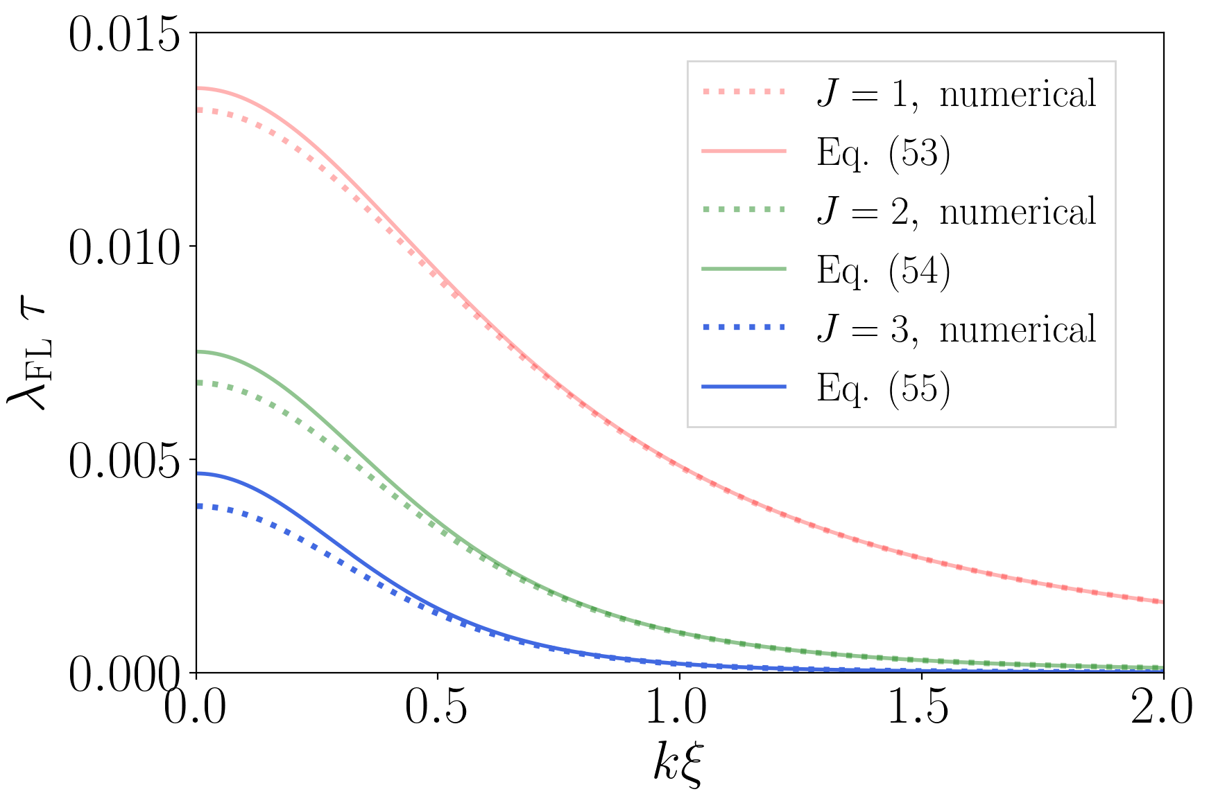
Although we can calculate $\lambda_{\mathrm{FL}}$ for higher $J$ in a similar manner as in the cases of $J=1$ and 2, it requires tedious calculations. We note that $\lambda_{\mathrm{FL}}$ at $\hbar\Omega=2E_{k}/J$ can be obtained more easily by using the conventional perturbation theory for degenerate states. We regard $b$ as a small perturbation parameter and rewrite Eq. $(\ref{eq:EigenEq})$ in the following form:

where $\hat{E}$ and $b\hat{V}$ are the matrices composed of the diagonal and off-diagonal elements of $\hat{Q}$, respectively. As we have discussed in the above, at $\hbar\Omega=2E_{k}/J$, the states $\ket{C_{j,+}}$ and $\ket{C_{j+J,-}}$ are degenerate at $b=0$. These states are coupled in the $J$th order perturbation, giving rise to a nonzero $\lambda_{\mathrm{FL}}$. Following the conventional perturbation theory for degenerate states, $\lambda_{\mathrm{FL}}$’s for $J=1,2$ and $3$ are obtained as the imaginary parts of the eigenvalues of the $2\times 2$ matrices, respectively, given by

where $l,l^{\prime}=(j,+)$ and $(j+J,-)$, and we take the summation over $l_{1},l_{2}=(j,s)$ for all possible combinations of $j\in\mathbb{Z}$ and $s=+$ and $-$ other than $(j,+)$ and $(j+J,-)$. The resulting FL exponents are given by

The results for $J=1$ and 2 coincide with Eqs. (78) and (121), respectively. We can calculate the FL exponent for $J\geq 4$ in the same manner, but we need to be careful that the diagonal terms of $V_{ll^{\prime}}^{(J^{\prime})}$ with even $J^{\prime}<J$ generally lifts the degeneracy of $(j,+)$ and $(j+J,-)$ states, which also contributes to $\mathrm{Im}\lambda_{\mathrm{F}}$ for $J=3$.

Figure 3 compares numerical results of $\lambda_{\mathrm{FL}}$ (dotted lines) with Eqs. (92)–(94) (solid lines). As one can see, the approximation works quite well for larger $k\xi$ because the perturbation parameter $b=q_{\mathrm{osc}}/2E_{k}$ becomes smaller for larger $k\xi$.

We solve Eq. (1) for a 1D system of a system size $L_{x}/\xi=256$ with a periodic boundary condition. The initial wavefunction is given by

where $R_{m,l}(x)$ $(l=1,2)$ is a uniform random number in [0,1]. We choose the parameters as $(q_{0},q_{\mathrm{osc}},\hbar\Omega)=(0.5,0.39,2E_{k_{\mathrm{res}}})$ with $k_{\mathrm{res}}=10\times 2\pi/L_{x}$. According to Eq. (78), the $\Omega$ is the resonance frequency of $J=1$, and the spin waves with the wavelength $L_{x}/10$ will grow. The interaction parameters are set to be $c_{1}/c_{0}=1/20$ and $-1/20$ for AFM and FM BECs, respectively.

In Fig. 4, we plot the time evolution of the spin density $f_{x}(x,t)$ which is expected to grow as $e^{\lambda_{\textrm{FL}}t}$ within the linear analysis. Figures 4(a) and (b) show the spatial and temporal distributions of $f_{x}(x,t)$ for the AFM and FM systems, respectively. As expected from the linear analysis, the spin waves with wavelength $L_{x}/10$ grow in the early stage (see the enlarged views in Fig. 4). In the late stage ($t/\tau\gtrsim 1500$), $f_{x}(x,t)$ in the AFM system exhibits finer structure than that in the FM system. This can be seen more clearly in the $k$-space.

Figure 5 shows the dynamics in the $k$-space. Here, we define the Fourier components in the 1D system as $\tilde{A}(k)\equiv\int_{0}^{L_{x}}A(x)e^{-ikx}dx$ and plot $|\tilde{f}_{x}(k,t)|^{2}$ averaged over 1000 samples of random initial states given by Eq. (95). Figures 5(a1) and (a2) show the time evolution of $|\tilde{f}_{x}(k_{\mathrm{res}},t)|^{2}$ for the AFM and FM systems, respectively, where the dashed lines are the analytical result $e^{2\lambda_{\textrm{FL}}t}$ with $\lambda_{\textrm{FL}}$ given in Eq. (92). One can clearly see that, for both cases, $|\tilde{f}_{x}(k_{\textrm{res}},t)|^{2}$ in the early stage agrees well with the linear analysis.

The linear analysis breaks down in the long-time dynamics, and $|\tilde{f}_{x}(k_{\textrm{res}},t)|^{2}$ in Figs. 5 (a1) and (a2) deviates from the exponential growth. The breakdown of the linear analysis is also seen in the $k$ dependence of $|\tilde{f}_{x}(k,t)|^{2}$ shown in Fig. 5(b), where the results for AFM (FM) systems are shown with open (filled) circles. As one can see, in addition to the main peak at $k=k_{\textrm{res}}$, small peaks appear around odd multiples of $k_{\mathrm{res}}$ at $t/\tau=400$. They are consequences of the nonlinear effect as mentioned in the next subsection. As time evolves, these peaks become broader, and $|\tilde{f}_{x}(k,t)|^{2}$ eventually distributes in the wide range of $k$. Figure 5(b) directly shows that the sign of $c_{1}$ significantly alters the late dynamics especially at $t/\tau\geq 680$: The spectra of the AFM system have the larger values in the high wavenumber region than those of the FM system. This is consistent with the real space configuration of $f_{x}(x,t)$ in Fig. 4.

References

- Bukov et al. (2015) M. Bukov, L. D’Alessio, and A. Polkovnikov, Advances in Physics 64, 139 (2015).
- Eckardt (2017) A. Eckardt, Rev. Mod. Phys. 89, 011004 (2017).
- Oka and Kitamura (2019) T. Oka and S. Kitamura, Annual Review of Condensed Matter Physics 10, 387 (2019).
- Aidelsburger et al. (2013) M. Aidelsburger, M. Atala, M. Lohse, J. T. Barreiro, B. Paredes, and I. Bloch, Phys. Rev. Lett. 111, 185301 (2013).
- Miyake et al. (2013) H. Miyake, G. A. Siviloglou, C. J. Kennedy, W. C. Burton, and W. Ketterle, Phys. Rev. Lett. 111, 185302 (2013).
- Jotzu et al. (2014) G. Jotzu, M. Messer, R. Desbuquois, M. Lebrat, T. Uehlinger, D. Greif, and T. Esslinger, Nature 515, 237 (2014).
- Choi et al. (2017) S. Choi, J. Choi, R. Landig, G. Kucsko, H. Zhou, J. Isoya, F. Jelezko, S. Onoda, H. Sumiya, V. Khemani, C. von Keyserlingk, N. Y. Yao, E. Demler, and M. D. Lukin, Nature 543, 221 (2017).
- Zhang et al. (2017) J. Zhang, P. W. Hess, A. Kyprianidis, P. Becker, A. Lee, J. Smith, G. Pagano, I. D. Potirniche, A. C. Potter, A. Vishwanath, N. Y. Yao, and C. Monroe, Nature 543, 217 (2017).
- Qu et al. (2020) A. Qu, B. Evrard, J. Dalibard, and F. Gerbier, Phys. Rev. Lett. 125, 033401 (2020).
- Kawaguchi and Ueda (2012) Y. Kawaguchi and M. Ueda, Physics Reports 520, 253 (2012).
- Stamper-Kurn and Ueda (2013) D. M. Stamper-Kurn and M. Ueda, Rev. Mod. Phys. 85, 1191 (2013).
- Shapiro (1963) S. Shapiro, Phys. Rev. Lett. 11, 80 (1963).
- Evrard et al. (2019) B. Evrard, A. Qu, K. Jiménez-García, J. Dalibard, and F. Gerbier, Phys. Rev. A 100, 023604 (2019).
- Stenger et al. (1998) J. Stenger, S. Inouye, D. M. Stamper-Kurn, H. J. Miesner, A. P. Chikkatur, and W. Ketterle, Nature 396, 345 (1998).
- Sadler et al. (2006) L. E. Sadler, J. M. Higbie, S. R. Leslie, M. Vengalattore, and D. M. Stamper-Kurn, Nature 443, 312 (2006).
- Ho (1998) T.-L. Ho, Phys. Rev. Lett. 81, 742 (1998).
- Ohmi and Machida (1998) T. Ohmi and K. Machida, Journal of the Physical Society of Japan 67, 1822 (1998).
- Yukawa and Ueda (2012) E. Yukawa and M. Ueda, Phys. Rev. A 86, 063614 (2012).
- Eto et al. (2018) Y. Eto, H. Shibayama, H. Saito, and T. Hirano, Phys. Rev. A 97, 021602 (2018).
- Kim et al. (2020) J. H. Kim, D. Hong, and Y. Shin, Phys. Rev. A 101, 061601 (2020).
- Vinit et al. (2013) A. Vinit, E. M. Bookjans, C. A. R. Sá de Melo, and C. Raman, Phys. Rev. Lett. 110, 165301 (2013).
- Jiménez-García et al. (2019) K. Jiménez-García, A. Invernizzi, B. Evrard, C. Frapolli, J. Dalibard, and F. Gerbier, Nature Communications 10, 1422 (2019).
- Huh et al. (2020) S. Huh, K. Kim, K. Kwon, and J.-y. Choi, Phys. Rev. Research 2, 033471 (2020).
- Hoang et al. (2016) T. M. Hoang, M. Anquez, B. A. Robbins, X. Y. Yang, B. J. Land, C. D. Hamley, and M. S. Chapman, Nature Communications 7, 11233 (2016).
- Kato (1995) T. Kato, Perturbation Theory for Linear Operators (Springer; 2nd ed., New York, 1995).
- Chen et al. (2019) T. Chen, K. Shibata, Y. Eto, T. Hirano, and H. Saito, Phys. Rev. A 100, 063610 (2019).
- Salwen (1955) H. Salwen, Phys. Rev. 99, 1274 (1955).
- Shirley (1965) J. H. Shirley, Phys. Rev. 138, B979 (1965).
- Zakharov et al. (1992) V. E. Zakharov, V. S. L’vov, and G. Falkovich, in Kolmogorov Spectra of Turbulence I: Wave Turbulence, Springer Series in Nonlinear Dynamics, edited by V. E. Zakharov, V. S. L’vov, and G. Falkovich (Springer, Berlin, Heidelberg, 1992) pp. 83–143.
- Samuelis et al. (2000) C. Samuelis, E. Tiesinga, T. Laue, M. Elbs, H. Knöckel, and E. Tiemann, Phys. Rev. A 63, 012710 (2000).
- van Kempen et al. (2002) E. G. M. van Kempen, S. J. J. M. F. Kokkelmans, D. J. Heinzen, and B. J. Verhaar, Phys. Rev. Lett. 88, 093201 (2002).
- Chai et al. (2020) X. Chai, L. You, and C. Raman, arXiv:2011.11462 (2020).