Magnetic topology in coupled binaries, spin-orbital resonances, and flares

As discussed above, the key point to production of observable flares is the establishment of quasi-steady magnetic configuration, whereby the magnetic energy is slowly stored in the magnetospheres and later released in a sudden flare.

There are several basic cases where we expect that the whole interacting magnetospheres periodically return to their initial state. Consider first the case of magnetic moments parallel to the $z$-axis (one aligned, one counter-aligned, so that the two stars are magnetically connected) and spins also (anti)/parallel to $z$. Case-I is a fully locked case: $\omega_{1}=\omega_{2}=\Omega$. In the rotating frame this corresponds to $\omega_{1}^{\prime}=\omega_{2}^{\prime}=0$ (dashed quantities are measured in the corotating frame). Neutron stars are not expected to be tidally locked (Bildsten & Cutler 1992), so this case is unlikely to be realized and, consequently, of no interest for us.

Case-II is counter-aligned spins in the corotating frame $\omega_{1}^{\prime}=-\omega_{2}^{\prime}$ (and arbitrary $\Omega$), Fig. 2. In this case in the rotating frame the configuration returns to the initial state. In the observer frame this corresponds to the case when the frequency of beat-plus of spins equals two times the orbital frequency, Figs. 3 and 4,

Importantly, the condition (1) applies to the beat-plus frequency $\omega_{1}+\omega_{2}$, not each individual frequency separately. We call this 2:1 resonance: the sum of spins is two times the orbital frequency, Fig. 3. This is the Dirac belt configuration. In the case of merging neutron stars the changing orbital frequency may, at some point, become two times the sum of spins.

To the best of our knowledge the 2:1 spin-orbital resonance has not been applied to magnetic fields of interacting binaries. In general physics such twisting arrangement is known under the names of “Dirac’s belt” or “Feynman arrow” (also related to a “Plate trick”).

In addition to the basic scenarios considered above, there is a number of more complicated cases. As we are about to demonstrate, the 2:1 resonance is more generic than the aligned case - it occurs for a wide variety of directions of spins and orbital axes and orientations of the intrinsic magnetic dipole moments. We shall now describe three indicative cases, illustrating them in Figs. 4-8 using table-top demonstrations. In the next section, we give a more economical description of the relevant geometry, and use it to revisit these illustrative cases again with better insight.

We number the two stars, let the first star not rotate at all, and, for definiteness, in all cases let the magnetic moments be counter-aligned along the $z$-axis at the initial moment (so that there is a strong magnetic coupling). Consider first when the spin of the second star is along the $x$ axis. Curiously, if the second star make one spin rotation first, then half an orbit, then another full spin rotation, and then another half an orbit, the configuration does not unwind, Fig. 5.

If, instead, the second star first makes two spin rotations, and then a full orbital rotation, the configuration doest unwind, Fig. 6. This example illustrates that the significance of the relative phase and angles.

Next, consider the case of spin of the second star along the $y$ axis. This case displays another property: topological bifurcation. In example in Fig. 7 the configuration unwinds, while in nearly equivalent case Fig. 8 it does not. Fig. 9 illustrates this behavior.

Let us start with a convenient mathematical description of a magnetic tube, it is a sufficiently small tubular neighborhood of some central magnetic line. It is formed by a smooth family of nearby magnetic lines parameterized by any transverse disk. (Mathematically, following the lines gives a diffeomorphism between any two transverse disks.)

Consider a pair of disks¹¹ 1 For global considerations $D_{1}$ is the magnetic North cap of star 1 and $D_{2}$ is the magnetic South cap of star 2. For local considerations, these are small star surface disks centered on the beginning and end of some central magnetic line. $D_{1}$ and $D_{2}$ (on the respective star surfaces) each oriented by a unit normal $\vec{\mu}_{1}$ and $\vec{\mu}_{2}$ directed along the magnetic field as in Figure 10. Their centers are connected by a length-parameterized path (representing a magnetic field line), the central line,

with unit tangent $\hat{B}=\frac{d\beta}{ds}$. A nearby magnetic field line (dashed green) intersects a normal disk centered at $\beta(s)$ at some point $\beta(s)+n(s)$ and thus the shape of the nearby line is determined by a normal vector field $n(s).$ Since we are only concerned with twisting, we keep track of the direction unit normal vector field $\hat{n}(s)=n(s)/|n(s)|.$ We shall be concerned with how much one line twists around the other, or, rather, how this twisting is changing with time, as the two discs orbit each other while also spinning at the same time.

For now let us focus on the static situation and describe the topology and geometry of a single magnetic tube, represented by a framed path $(\beta,\hat{n})$ with given initial and final frames specified by fixed $\hat{B}(0)=\vec{\mu}_{1},\hat{B}(\ell)=\vec{\mu}_{2},$ and fixed $\hat{n}(0)=\hat{n}_{1}$ and $\hat{n}(\ell)=\hat{n}_{2}$.

The frame along a path $\beta$ is specified by a single normal field $\hat{n}(s)$. Of course the complete frame is formed by the triplet of vectors $f=(\hat{B},\hat{n},\hat{B}\times\hat{n}).$ Written as a $3\times 3$ matrix, with each column representing a vector in this frame, we have an orthogonal matrix, thus a framed path gives a corresponding path in $SO(3)$ with

Thus, thinking of a small magnetic tube as a framed path we arrive at a path $f$ in $SO(3)$. Clearly, the first column of $f(s)$ is $\hat{B}(s)$, thus, the path $\beta$ can be recovered from $f$ via integration $\beta(s)=\beta(0)+\int_{0}^{s}f(s)(1,0,0)^{T}ds$.

Given two such framed paths $(\beta,\hat{n})$ and $(\beta^{\prime},\hat{n}^{\prime})$ with the same initial and final frames, one might ask whether it is possible to deform one of them into another, while holding the initial and final frames fixed. If it is indeed possible, then the corresponding paths $f$ and $f^{\prime}$ in $SO(3)$ are called homotopic. Thus it is worth understanding the space of paths in the group of orientation preserving rotations $SO(3).$ Any rotation of $\mathbb{R}^{3}$ can be specified by a single vector: its direction specified by the (oriented) axis of rotation and its length is the angle of the rotation around this axis. In particular the length of this vector does not exceed $\pi$. At this stage all rotations appear to be in one-to-one correspondence with a radius $\pi$ ball in $\mathbb{R}^{3},$ except for one caveat. A rotation by angle $\pi$ around $\hat{m}$ produces the same result as a rotation by $\pi$ around $-\hat{m},$ therefore the antipodal points on the surface of this ball correspond to the same rotation. One concludes that the group of rotations $SO(3)$ is a three-ball with antipodal points of its surface identified.

One can view this three-ball as a Northern hemisphere of some three-sphere $S^{3}$, making clear the identification of $SO(3)$ with the three-dimensional projective space $\mathbb{R}P^{3}=S^{3}/\{\pm 1\}$, which is a three-sphere with its antipodal points identified (or, equivalently, the space of lines in $\mathbb{R}^{3}$ passing through the origin): $\mathbb{R}P^{3}=SO(3)$.

While a three sphere is simply connected, i.e. any two paths between two given points can be deformed into each other. The projective space has exactly two classes of paths. The difference between the two paths is a closed path obtained by traversing the first path and then returning backwards along the second path. This difference between the two paths in different classes is homotopic to (i.e. can be deformed to) the path in $S^{3}$ connecting two of its antipodal points.

Note: the above is often illustrated with a belt, with its two ends held fixed at a distance, so that one can move the belt around these ends increasing or decreasing its twisting in the process. However, if one breaks the rules and twists one of the ends once, the resulting belt configuration differs from all prior ones, in that those cannot be reached by manipulating the belt, while its ends are held fixed.

The above correspondence is often interpreted in terms of spin. Namely, identifying $SU(2)$ as a three-sphere (for example, as a sphere of unit quaternions), and thinking of the three space $\mathbb{R}^{3}$ as imaginary quaternions, the rotation $R(M)$ of $\mathbb{R}^{3}$ is a conjugation of the imaginary quaternions by a unit quaternion: $SU(2)\ni M:x\mapsto M^{-1}xM$. Then, clearly, $M$ and $-M$ have exactly the same effect on $\mathbb{R}^{3}$ and the group of all orientation preserving rotations $SO(3)=SU(2)/\{\pm 1\}$. A framed path gives a path in $SO(3)$ (for example starting at identity and arriving at some fixed frame $M\in SO(3)$) and lifts unambiguously to a path in $SU(2)$ (also beginning at identity). It will arrive at some element of $\hat{M}\in SU(2)$. As we deform the path in $SO(3)$, its lift to $SU(2)$ will still be beginning at identity and ending at $\hat{M}.$ However, there is a whole other class of paths in $SO(3)$ to $M$, they lift to paths in $SU(2)$ from identity to $-\hat{M}$. Thus what governs the framed path (up to its deformations) is the spin group $Spin(3)=SU(2),$ rather than $SO(3).$ This is the reason a belt is sometimes used to illustrating fermion statistics.

Perhaps, a more economical view of a framed path is in terms of the tangent bundle $TS^{2}$ of a two-sphere of directions $S^{2}.$ This bundle consists of disjoint tangent planes to $S^{2}$. Namely, for any length parameterized path $\beta$ in $\mathbb{R}^{3}$, its normal tangents $\hat{B}:[0,\ell]\to S^{2},s\mapsto\hat{B}(s)=\frac{d}{ds}\beta(s)$ form a path in the unit sphere $S^{2}$ of directions, as in Fig.11, while $\hat{n}(s)$, orthogonal unit vector to $\hat{B}(s)$, is a tangent vector to $S^{2}$ at $\hat{B}(s)$ as in Fig. 12. Since it is normalized, it lies in the unit circle in the tangent plane $T_{\hat{B}(s)}S^{2}$ to $S^{2}$ at point $\hat{B}(s).$

Thus we arrive at a slightly different picture of the space $\mathbb{F}$ of all unit circles in the tangent spaces of the unit two-sphere: $\mathbb{F}=T^{1}S^{2}\subset TS^{2}.$ An element of this space is specified by a pair $(a,b)$ of orthogonal unit vectors, the first vector $a$ specifies the point in $S^{2}$ and the second vector $b$ specifies a point in the tangent plane to $S^{2}$ at $a.$ Of course, given a point $(a,b)\in\mathbb{F}$ the forgetful map $(a,b)\mapsto a$ gives the corresponding element of the sphere, in other words we have a natural projection $\mathbb{F}\to S^{2},(a,b)\mapsto a$ (it projects a circle fiber of normals to its corresponding point on the sphere of directions).

A framed path $(\beta,\hat{n})$ gives a path $\hat{\beta}$ in $\mathbb{F}$ by

The path in the sphere traced by $\hat{B}(s)$ simply traces out the directions of the path $\beta,$ while the unit tangent field $\hat{n}(s)$ along this path lifts it to $\mathbb{F}.$ The path in the sphere begins at $\vec{\mu}_{1}$ and ends in $\vec{\mu}_{2}.$ It is constrained by $\vec{R}=\int_{0}^{\ell}\hat{B}(s)ds.$ Thus, this path is bound to spend some time near $\vec{R}/|\vec{R}|\in S^{2},$ as illustrated in Figure 11. Needless to say, our description is equivalent to that of section IV.2, as the space $\mathbb{F}$ can be identified with $SO(3)$ via $(a,b)\mapsto(a,b,a\times b).$

Let us comment on the topology of the unit circle bundle $T^{1}S^{2}$ of the two-sphere $S^{2}$. In particular, we would like to make it transparent that it is a degree 2 Hopf bundle. This degree 2 is at the heart of the effect discussed in this paper; it is responsible for the persistence of the 2:1 resonance. Perhaps the most common way to demonstrate that the degree is 2 is to consider the polar projection $F:S\setminus\{N\}\to\mathbb{R}^{2}$ from the North pole $N$ to the plane tangent at the South pole $S$. Taking a constant vector field on the plane and pulling it back to $S\setminus\{N\}$ one obtains a vector field that winds twice as one circumnavigates the North pole traversing a small meridian near it.

For our purposes, however, we use a different picture. We trivialize the bundle over the Northern hemisphere $U_{N},$ the southern hemisphere $U_{S},$ and over the tropical region $U_{T}=S^{2}\setminus\{N,S\}$ containing the equator, as follows. Let us mark a point $E$ on the equator and call it the East pole. We also call its antipodal point the West pole. A unit tangent vector field $u$ directed towards $E$ is then well defined everywhere on the sphere except at $E$ and at $W$. We use it to define coordinates in the tangent circle fiber over $U_{N}$ and $U_{S}.$ For any point $p\in U_{N}$ and for any tangent unit vector $w_{p}$ at $p$, let $\phi_{N}(w_{p})$ be the angle between $u_{p}$ and $w_{p}$. Now, any real number determines a unique unit tangent vector at $p$, whose angle with $u_{p}$ is that number. In other words we defined a coordinate along the circle fiber. Similarly, if $p\in U_{S},$ we define $\phi_{S}(w_{p})$ to be the angle between $u_{p}$ and $w_{p}.$

Next, consider the Northward unit tangent field $v$. It is well defined everywhere in the tropical region $U_{T}$. For any $p\in U_{T}$ let $\phi_{T}(w_{p})$ be the angle between $v_{p}$ and $w_{p}.$

Consider some parallel in the Northern hemisphere and a point $p$ on it. Clearly, $\phi_{T}=\phi_{N}+\phi_{T}(v_{p}),$ i.e. the difference between the two angles $\phi_{T}(w_{p})$ and $\phi_{N}(w_{p})$ is the angle between $v_{p}$ and $u_{p}$. Whenever the point $p$ circumnavigates the parallel Eastward, this angle between $v_{p}$ and $u_{p}$ changes by $2\pi$, i.e. $\Delta(\phi_{T}(w_{p})-\phi_{N}(w_{p}))=2\pi.$ Similarly, circumnavigating any parallel in the Southern hemisphere Eastwards, the change in the difference between $\phi_{T}$ and $\phi_{S}$ is $-2\pi,$ i.e. $\Delta(\phi_{T}(w_{p})-\phi_{S}(w_{p}))=-2\pi.$

For example, if we have a path in $\mathbb{F}$ passing over the equator, then, if we move it all the way around the equator holding the limiting value of, say, $\phi_{N}$ at the equator fixed, then the value of $\phi_{E}$ will change by $2\pi,$ while the value of $\phi_{S}$ will change by $4\pi.$ It is this factor of 2 in $2\times 2\pi$, that is the degree or the Hopf number of this bundle. (It is exactly because this degree is not zero that the sphere ‘cannot be combed’, i.e. it has no nowhere vanishing continuous tangent fields. It is also the reason there is no global coordinate along the fiber of $\mathbb{F}$.)

For some paths one might be able to introduce the notion of twisting, for example, using the (unit) tangent $\hat{B}$ and curvature $d\hat{B}/ds$ of the path to form a frame along it. Such a Frenet frame could be used to define the twisting of a magnetic tube centered around that path. However, as we consider the evolution of the path, as it changes its shape we might (and even are likely to) loose this frame. For example, the curvature might vanish at some point. This would prevent continuous tracking of this path twisting angle. In other words, there are two issues preventing us from discussing twisting of an arbitrary tube:

1. 1.

   there cannot be a coordinate on the fiber circle that is valid over the whole sphere of directions and

2. 2.

   there is no guarantee that the path of directions $\hat{B}$ is differentiable, even though the original path in $\mathbb{R}^{3}$ was.

However, if we have one path $\hat{\gamma}_{1}$ and another path $\hat{\gamma}_{2}$ in $T^{1}S^{2},$ and both happen to project to the same path $\gamma$ in $S^{2},$ then there is a good notion of how much $\hat{\gamma}_{2}$ winds around $\hat{\gamma}_{1}.$ To do this, as we traverse $\gamma$, we continuously track the change in the angle between $\hat{\gamma}_{1}(s)$ and $\hat{\gamma}_{2}(s)$. Importantly, this does not involve any charts, fiber coordinates, or auxiliary vector fields. Thus, for such pair of paths the relative twisting angle is well defined.

In general we shall consider a family of framed paths $\hat{\gamma}(s,t)$, where $s$ is the length parameter along a path at time $t$. In particular, $\hat{\gamma}(s,0)=\hat{\gamma}_{1}(s)$ is the initial path and $\hat{\gamma}(s,2\pi)=\hat{\gamma}_{2}(s)$ is the final path. Also, the projection of $\hat{\gamma}(s,t)\in\mathbb{F}$ is the direction $\gamma(s,t).$

Let us begin with a very simple example, consider a path $\gamma(s,t)$ that is the meridian from $N$ to $S$ with longitude $t$. Clearly, as $t$ changes from $0$ to $2\pi$ this meridian sweeps the sphere and returns to its original shape, i.e. $\gamma(s,0)=\gamma(s,2\pi).$ Consider a tangent vector field to each meridian that, away from a small neighborhood of the equator is given by the East pole directed field $v$. (Clearly, the field $v$ does not give a good normal field along the whole family $\gamma(s,t)$, since it is not defined at $E$ and $W$. Thus, for each $t$ we interpolate the resulting tangent field along the path $\gamma(s,t)$ in the vicinity of the equator.) Let $\hat{\gamma}(s,0)$ be the path lifting the meridian $\gamma(s,0)$ using that field (outside the neighborhood of the equator) and continuous along the whole meridian. As we vary $t$ and the meridian $\gamma(s,t)$ rotates sweeping the sphere, we keep $\hat{\gamma}(s,t)$ given by $v$ away from the equator and change continuously with $s$ and $t$. We would like to learn about the resulting path $\hat{\gamma}(s,2\pi)$ relation to the original path $\hat{\gamma}(s,0).$

In terms of the local coordinates, these paths have $\phi_{N}=0$ and $\phi_{S}=0$ away from the neighborhood of the equator. There is a discontinuity between $\phi_{N}$ and $\phi_{T}$, for example, and this discontinuity changes by $2\pi$ as the meridian sweeps the sphere. Since we keep the North and South coordinates zero by construction, and the gap between $\phi_{N}$ and $\phi_{T}$ changes by $2\pi$, the interpolating path near equator has to adjust, changing its initial value of $\phi_{T}$ just North of equator. Similarly, since the gap between $\phi_{T}$ and $\phi_{S}$ changes by $2\pi$, the value of $\phi_{T}$ just South of the equator changes. As a result, the interpolating part of the path shown in dashed blue in Fig. 14 wraps twice around the fiber relative to the original path shown in solid red.

In fact, nothing in this argument depends on our special choice of path lifting, so long as we hold the initial and final frames fixed. (The solid red and dashed blue graphs in Fig. 14 will be arbitrary, but the relation between their discontinuities will remain the same, adding up to $4\pi$.) As the path $\gamma$ sweeps the sphere once (moving Eastwards), the path $\hat{\gamma}(s,2\pi)$ will twist by $4\pi$ relative to $\hat{\gamma}(s,0).$

With our newly gained perspective let us revisit the cases discussed in Sec. III and account for the observed twisting.

Case I had $\vec{\omega}_{1}=\vec{\omega}_{2}=\vec{\Omega}\sim\hat{z}$. In terms of the sphere of directions this can be visualized, left Fig. 15, as points $\vec{\mu}_{1}$ and $\vec{\mu}_{2}$ presented as, respectively, red and blue dots circling in the same (Eastward) direction around, respectively, North and South poles. The path of directions is the blue path on the sphere connecting these two points and passing in the vicinity of the black dot $\hat{R}$. The latter rotates around the equator. The twisting is captured by the sum of the angles $\chi_{1}$ and $\chi_{2}.$ For Case I all three points (red, blue, and black) rotate with the angular velocity, and the resulting angles $\chi_{1}$ and $\chi_{2}$ can remain constant. Therefore, we observe no winding.

Case II, as illustrated in Fig. 2, is very similar to the picture above. As illustrated in the right Fig. 15, the red and blue dots moving in the opposite directions (with equal angular velocity), while the black bot is staying put. In this case one of the $\chi$ angles increases, while another decreases, with their sum remaining constant (on average). Therefore, there cannot be twisting in this case.

Case II, as illustrated in Fig. 3, is the picture we just described, but rotated, so that now the blue dot is staying put, the black dot rotates, and the red dot rotates twice as fast. This modification has no bearing on the resulting evolution of the angles $\chi_{1}$ and $\chi_{2}$, again resulting in no winding.

In the remaining cases, Figs. 5-8, $\vec{\omega}_{1}=0$ and the red dot stays put at the North pole. Clearly, for actual continuous spin and orbital motions there is no difference between $\vec{\omega}_{2}$ directed along $x$- or along $y$-axis, due to the rotational symmetry. In the table-top demonstrations, however, the motions are consecutive and the result depends on their order. For example, Fig. 5 movements in terms of the direction two-sphere on the left of Fig. 16, amount to the blue point circling along the vertical meridian (winding=-1), then the original black dot $\hat{R}(1)$ moving along the equator to $\hat{R}(3)$ (winding=-1+1), the blue point circles the meridian again (with $\hat{R}$) on the other side (winding=-1+1+1), and the blue point completes its journey around the equator (winding=-1+1+1+1).

The movements of Fig. 6, on the other hand, consist of the blue point circling the meridian twice (winding=-2) followed by the black dot circling the equator (winding=-2+2).

The case of $\vec{\omega}_{2}$ aligned with the $y$-axis presents a bifurcation, since in this case the blue point passes through the black point. This is the moment of bifurcation. Movements of Fig. 8 (with $\vec{\omega}_{2}=\omega_{2}\hat{y}+\epsilon\hat{x}$) from the direction two-sphere point of view are not so different from those of Fig. 5 discussed above. The only difference is that the vertical meridian is rotated to the green meridian in Fig. 16. The winding calculation remains the same.

Movements of Fig. 7 result in blue point circling the green meridian (winding=-1), black point moving along the equator from $\hat{R}(1)$ to $\hat{R}(2)$ (winding=-1+1), then the blue point circling the orange meridian (winding=-1+1-1), and the black point completing its trip around the equator (winding=-1+1-1+1).

If we keep the central line fixed and rotate the first disk in Fig. 10 around its axis once, the new green path will wind by $2\pi$ relative to the original green path. Similarly, rotating the second disc once winds this path by $-2\pi$. All the action in these cases is taking place in the cylinder in $\mathbb{F}=T^{1}S^{2}$ that is the preimage of the blue direction path.

Another important effect is due to the orbital motion, namely the point $\hat{R}=\vec{R}/|\vec{R}|$ is rotating around the equator with frequency $\Omega.$ Let us first focus on the path of directions in the sphere $S^{2}$ while holding its origin $\vec{\mu}_{1}$ and its end $\vec{\mu}_{2}$ fixed. Moreover, we presume that $\vec{\mu}_{1}$ is in the Northern hemisphere and $\vec{\mu}_{2}$ is in the Southern hemisphere. As discussed in Sec. IV.3, the path of directions passes in vicinity of $\hat{R}$, as illustrated in Fig. 11. As a result, during one orbital rotation the path of directions sweeps the whole surface of the sphere, and the magnetic tube twisting angle will increase by $4\pi$ with each such sweep.

Since the main phenomenon we are describing is topological in nature, we can simplify our path of directions by deforming it to be the major arc from $\vec{\mu}_{1}$ to $\hat{R}$ followed by the major arc from $\hat{R}$ to $\vec{\mu}_{2}$. (For example we can deform the blue path of directions to the arc path just described, without passing through the antipodal point $-\hat{R}.$) During this deformation the covering path (dashed blue) will deform as well. In fact, we deform it so that at $\hat{R}$ the tangent vector is pointing due North. Any such choice does not change the twisting, since rotating the tangent vector at $\hat{R}$ by some angle $\phi$ twists one part of the tube by $-\phi,$ while twisting the other by $\phi,$ thus not changing the total path twisting at all.

This deformation makes it very easy to track the tube winding and its time evolution. In fact, now that the frame at $\hat{R}$ is fixed, we have a separate notion of twisting of the first part of the path and of its second part. In particular, if $\vec{\mu}_{1}\in U_{N}$ and $\vec{\mu}_{2}\in U_{S}$, then as $\hat{R}$ circumnavigates the equator, the Northern part winds by $2\pi$, and so does the Southern part. Let us put this more geometrically. When the point $\hat{R}$ rotates around $\vec{\mu}_{1}$ counterclockwise, the $\vec{\mu}_{1}-\hat{R}$ path segment is twisted by $2\pi.$ Similarly, whenever, $\hat{R}$ moves around $\vec{\mu}_{2}$ clockwise the segment $\hat{R}-\vec{\mu}_{2}$ is twisted by $2\pi.$ (Note, the difference is due to the opposite orientation: $\vec{\mu}-\hat{R}$ vs $\hat{R}-\vec{\mu}$.)

Now, as the path of directions returns to itself after one orbital rotation, what happens to the magnetic flux tube? It is twisted by $4\pi$ if $\vec{\mu}_{1}$ is North of equator and $\vec{\mu}_{2}$ is South of it. It is twisted by $-4\pi$ if $\vec{\mu}_{1}$ is South of equator and $\vec{\mu}_{2}$ is North of it. And it is not twisted at all if $\vec{\mu}_{1}$ and $\vec{\mu}_{2}$ are on the same side of the equator. This effect of the orbital motion is due to the fact that the bundle $\mathbb{F}$ of circles over the sphere has Hopf number 2.

Of course in general the disks will spin and orbit each other at the same time. Consider the first disk rotating with angular velocity $\vec{\omega}_{1}$ and the second with angular velocity $\vec{\omega}_{2}.$ Then, the points $\vec{\mu}_{1}$ and $\vec{\mu}_{2}$ will be in circular motions around $\hat{\omega}_{1}=\frac{\vec{\omega}_{1}}{\omega_{1}}$ and $\hat{\omega}_{2}=\frac{\vec{\omega}_{2}}{\omega_{2}}$ respectively. Let $\alpha_{1}$ be the angle between $\vec{\Omega}$ and $\vec{\omega}_{1}$ and let $\beta_{1}$ be the angle between $\vec{\omega}_{1}$ and $\vec{\mu}_{1}$, as in Fig. 17. Similarly, we define $\alpha_{2}$ and $\beta_{2}$ using $\vec{\omega}_{2}$ and $\vec{\mu}_{2}$. Now, as the first disk undergoes one such rotation around $\omega_{1}$ it rotates around its axis once, therefore, as $\vec{\mu}_{1}$ undergoes one rotation around $\frac{\omega_{1}}{|\omega_{1}|}$ the circle fiber of $\mathbb{F}$ above it rotates once (relative to the fiber at $\hat{\omega}_{1}$). The resulting twisting, however, depends on whether $\vec{R}$ lies inside or outside the smaller disk bounded by the circle traversed by $\omega_{1}$ (or, respectively, $\omega_{2}$).

If the motion of $\vec{\mu}_{1}$ is happening entirely in one hemisphere (either Northern or Southern) and the same holds for $\vec{\mu}_{2},$ then the twisting rate of the $\hat{\mu}_{1}-\hat{R}$ part is $-\omega_{1}\,\mathrm{sign}\,\vec{\omega}_{1}\cdot\vec{\mu}_{1}+\Omega\,\mathrm{sign}\vec{\Omega}\cdot\vec{\mu}_{1}$, while the twisting rate of the $\hat{R}-\hat{\mu}_{2}$ part is $-\omega_{2}\,\mathrm{sign}\,\vec{\omega}_{2}\cdot\vec{\mu}_{2}+\Omega\,\mathrm{sign}\vec{\Omega}\cdot\vec{\mu}_{2}.$ Assembling the two together we have the rate of twisting of the whole path:

The above holds so long as $\alpha_{i}+\beta_{i}<\frac{\pi}{2}$ or after $\alpha_{i}-\beta_{i}>\frac{\pi}{2}$ for $i=1,2$. Otherwise the circle on the direction sphere that $\vec{\mu}_{i}$ traces out dips in the other hemisphere. What fraction of this circle is in the other hemisphere? In other words, how long is the arc between the two points $O$ and $O^{\prime}$ (see Fig. 17) at which $\vec{\mu}_{1}$ passes the equator?

Let $\delta_{1}=\frac{\pi}{2}-\alpha_{1}$ be the latitude of $\vec{\omega}_{1}.$ Then from the spherical triangle formed by $\vec{\omega}_{1},$ $O,$ and the equator midpoint $M$ between $O$ and $O^{\prime}$ we have

Thus $\sin A=\frac{\sqrt{\sin^{2}\alpha_{1}-\cos^{2}\beta_{1}}}{\sin\alpha_{1}\sin\beta_{1}},$ and the fraction of the $\vec{\mu}_{1}$ circle that is in the opposite hemisphere is

Assuming for a moment that the rotation frequencies are much higher than the orbital frequency: $\omega_{1},\omega_{2}\gg\Omega,$ the average twisting rate $\mathcal{R}$ is

Here $f_{j}=f(\alpha_{j},\beta_{j})$ given by Eq. 9 with $\alpha_{j}$ being the angle between $\vec{\Omega}$ and $\vec{\omega}_{j}$ and $\beta_{j}$ angle between $\vec{\omega}_{j}$ and $\vec{\mu}_{j}.$

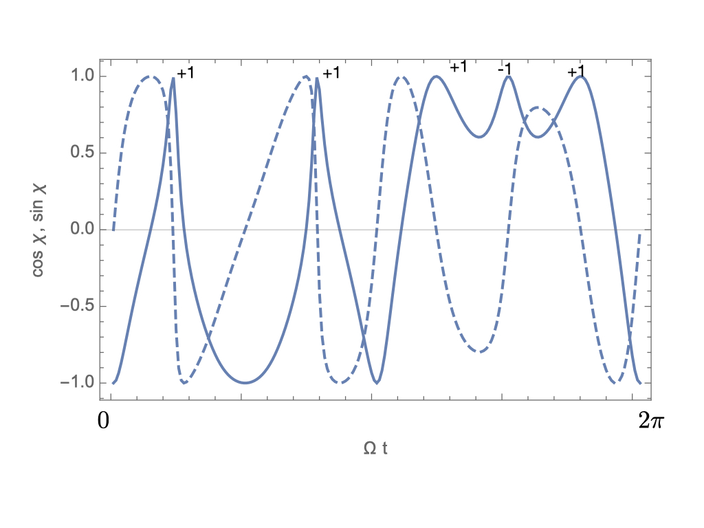
This provides the average rate of winding of the magnetosphere for the general relative orientation of spins and orbital angular velocity. The averaging used applies whenever $\omega_{1},\omega_{2}\gg\Omega.$ Fig. 20 illustrating the time average converging to $\mathcal{R}.$ Whenever the spins and angles are such that this rate $\mathcal{R}$ is low, a slow winding of the magnetosphere is possible on average over time. This does not imply, however, that these configurations allow for gradual storage of energy in the magnetosphere, since the critical winding might/is likely to be breached in the interim. With this in mind we focus on identifying other possible resonances.

We can have multiple non-winding resonances besides the 2:1 resonance; but their appearance depends on the phase. Thus, in a given system one can observe several various resonances. These higher resonances however are much less stable.

Consider a snapshot with $\omega_{1},\hat{R}=M,$ and $\vec{\mu}_{1}$ aligned lying on a spherical radius of the blue disk in Fig. 17. If in the near future $\hat{R}$ reaches point $O$ before $\vec{\mu}_{1}$ does, then it also implies that in the recent past $\vec{\mu}_{1}$ passed through point $O^{\prime}$ before $\hat{R}$ did. In other words, the motion of $\vec{\mu}_{1}$ over the arch $O^{\prime}O$ canceled the effect of $\hat{R}$ traversing the equator. (I.e. $\vec{\mu}_{1}$ made one clockwise rotation around $\hat{R}$.)

The necessary condition for such occurrence is $\frac{a}{\Omega}<\frac{A}{\omega}$, which translates to

If the above snapshot occurs and the ration of the two frequencies is rational, the above snapshot will recur with regularity. E.g. if $\frac{\omega_{1}}{\Omega}=\frac{2}{3},$ then every two orbital periods $\vec{\omega}_{1},\hat{R},$ and $\vec{\mu}_{1}$ are aligned again and the orbital winding effect is compensated by the above maneuver. Therefore, the effective magnetic tube winding rate is $\omega_{1}-\Omega(1-\frac{1}{3})$, which vanishes. In particular, if it so happens that $\vec{\mu}_{2}$ is engaged in a similar resonant configuration, then the total winding rate is zero. To summarize, we have another resonant configuration

In contrast to $2:1$ resonance which was very stable with respect to changes of angles, phases, and frequencies, this $4:3$ resonance is sensitive not only to angles and frequencies, but even to the phase, i.e. to the particular momentary (approximate) alignment. Nevertheless, during the binary evolution such resonances can occur. Moreover, there are many other possible resonances. If they are observed, they can provide detailed information about the individual spins, their orientations, and about the orbital frequency.

Let us estimate the local region of magnetosphere that can contribute to the 4:3 resonance. The $\hat{R}$ transit time (between $O^{\prime}$ and $O$) is $T_{R}=\frac{2a}{\Omega}$. The angular distance traveled by $\hat{B}$ during this time is $\omega T_{R}=\frac{\omega}{\Omega}2a.$ The remaining angular span of the $O^{\prime}O$ arc (on the boundary of the blue spherical disk in Fig. 17) is therefore $2A-\frac{\omega}{\Omega}2a$. This is the arc of the $\hat{B}$ points involved in the above described behavior leading to the 4:3 resonance. I.e. a point $\hat{B}$ passes $O^{\prime}$ before $\hat{R}$ does, and then $\hat{B}$ passes $O$ after $\hat{R}$ does. Thus, for each value of $\beta$ there is an arc of angular size

The relevant solid angle formed by the magnetic line star surface directions involved in the resonance is

The upper limit is reached when the equatorial arc $O^{\prime}O$ spans one third of the equator, i.e. $2a<\frac{2\pi}{3}$, implying $\cos\beta<\frac{1}{2}\sin\alpha$.

Now the fragility of this resonance can be illustrated in Fig. 21. The resonant region, indicated in red, involves only those magnetic lines whose direction at the star surface lie in both the interacting magnetic polar cap (shown in cyan) and in the resonant (red) region. With our formulas above one can estimate how likely it is that these two regions intersect at all and what the maximal overlap of these two regions can be.

References

- Antoine (2021) Antoine, S. 2021, arXiv e-prints, arXiv:2104.05968
- Arnold (1974) Arnold, V. I. 1974, Proc. Summer School in Differential Equations, Erevan. Armenian SSR A d Sci.
- Arnold (1986) Arnold, V. I. 1986, Selecta Math. Soviet., 5, 327, selected translations
- Bildsten & Cutler (1992) Bildsten, L., & Cutler, C. 1992, ApJ, 400, 175
- Buckley et al. (2017) Buckley, D. A. H., Meintjes, P. J., Potter, S. B., Marsh, T. R., & Gänsicke, B. T. 2017, Nature Astronomy, 1, 0029
- Callister et al. (2019) Callister, T. A., et al. 2019, ApJ, 877, L39
- Cauley et al. (2019) Cauley, P. W., Shkolnik, E. L., Llama, J., & Lanza, A. F. 2019, Nature Astronomy, 3, 1128
- Goldreich & Julian (1969) Goldreich, P., & Julian, W. H. 1969, ApJ, 157, 869
- Hansen & Lyutikov (2001) Hansen, B. M. S., & Lyutikov, M. 2001, MNRAS, 322, 695
- Hut (1981) Hut, P. 1981, A&A, 99, 126
- Lyutikov (2011) Lyutikov, M. 2011, Phys. Rev. D, 83, 124035
- Lyutikov (2019) —. 2019, MNRAS, 483, 2766
- Moffatt & Dormy (2019) Moffatt, K., & Dormy, E. 2019, Self-Exciting Fluid Dynamos, Cambridge Texts in Applied Mathematics (Cambridge University Press)
- Most & Philippov (2020) Most, E. R., & Philippov, A. A. 2020, ApJ, 893, L6
- Palenzuela et al. (2013) Palenzuela, C., Lehner, L., Ponce, M., Liebling, S. L., Anderson, M., Neilsen, D., & Motl, P. 2013, Physical Review Letters, 111, 061105
- Radice et al. (2018) Radice, D., Perego, A., Hotokezaka, K., Fromm, S. A., Bernuzzi, S., & Roberts, L. F. 2018, ApJ, 869, 130
- Rubenstein & Schaefer (2000) Rubenstein, E. P., & Schaefer, B. E. 2000, ApJ, 529, 1031
- Sachdev et al. (2020) Sachdev, S., et al. 2020, ApJ, 905, L25
- Schaefer et al. (2000) Schaefer, B. E., King, J. R., & Deliyannis, C. P. 2000, ApJ, 529, 1026
- Shultz et al. (2015) Shultz, M., Wade, G. A., Alecian, E., & BinaMIcS Collaboration. 2015, MNRAS, 454, L1
- Tejada Arevalo et al. (2021) Tejada Arevalo, R. A., Winn, J. N., & Anderson, K. R. 2021, arXiv e-prints, arXiv:2107.05759
- Turner et al. (2021) Turner, J. D., et al. 2021, A&A, 645, A59
- Vedantham et al. (2020) Vedantham, H. K., et al. 2020, Nature Astronomy, 4, 577
- Warner (1983) Warner, B. 1983, in Astrophysics and Space Science Library, Vol. 101, IAU Colloq. 72: Cataclysmic Variables and Related Objects, ed. M. Livio & G. Shaviv, 155–171
- Winn & Fabrycky (2015) Winn, J. N., & Fabrycky, D. C. 2015, ARA&A, 53, 409