Study of pion vector form factor and its contribution to the muon $(g-2)$

The muon magnetic moment is an important and long historical issue in particle physics Garwin:1957hc; Garwin:1960zz; Terazawa:1968jh; Terazawa:1968mx; Terazawa:1969ih; Kinoshita:1970js; Terazawa:2018pdc. Using Dirac theory, the gyromagnetic ratio $g_{\mu}$ is predicted as $g_{\mu}=2$ for the structureless and spin $\frac{1}{2}$ muon. In fact, due to the developments of the experiments and theories, it is found that $g_{\mu}$ is slightly greater than 2, which can be referred to as the anomalous magnetic moment $a_{\mu}=(g_{\mu}-2)/2$. As already known, it is Schwinger’s value of $a_{\mu}=\alpha/(2\pi)\simeq 0.00116$ from one loop QED radiative corrections, which is universal for all leptons. More discussions for that can be found in the reviews of Jegerlehner:2009ry; Miller:2012opa. The anomalous magnetic moment of the muon $a_{\mu}$ is experimentally and theoretically known to very high accuracy. Its measurement at Brookhaven National Laboratory was reported as Bennett:2006fi; Mohr:2012tt

$$a_{\mu}^{\mathrm{exp}}=(11659209.1\pm 5.4\pm 3.3)\times 10^{-10},$$

(1)

where the errors were given by statistical and systematic uncertainties, respectively. The Standard Model (SM) prediction was given by Davier:2019can

$$a_{\mu}^{\mathrm{SM}}=(11659183.1\pm 4.0\pm 2.6\pm 0.1)\times 10^{-10}.$$

(2)

And thus, the difference between the experiment and theory is

$$\Delta a_{\mu}=a_{\mu}^{\exp}-a_{\mu}^{\mathrm{SM}}=(26.0\pm 7.9)\times 10^{-10},$$

(3)

where one can see that there is a discrepancy of about 3.3$\sigma$ between the measured value and the full Standard Model prediction. But, this discrepancy has been updated with the recent results both in theory calculations and experimental measurements. The latest measurement of the anomalous magnetic moment of the muon was performed at Fermilab National Accelerator Laboratory Muon $g-2$ Experiment Muong-2:2021hlp, gotten

$$a_{\mu}^{\mathrm{exp}}=(11659204.0\pm 5.4)\times 10^{-10}.$$

(4)

Combined with the measurement at Brookhaven above, one can easily get the experimental average of

$$a_{\mu}^{\mathrm{exp}}=(11659206.1\pm 4.1)\times 10^{-10}.$$

(5)

Note that the reported results of Ref. Bennett:2006fi were used for this average. The latest SM prediction was given by the recent review of the White Paper (WP) Aoyama:2020ynm

$$a_{\mu}^{\mathrm{SM}}=(11659181.0\pm 4.3)\times 10^{-10}.$$

(6)

Therefore, the difference between the experiment and the theory is updated as

$$\Delta a_{\mu}^{\mathrm{new}}=a_{\mu}^{\exp}-a_{\mu}^{\mathrm{SM}}=(25.1\pm 5.9)\times 10^{-10},$$

(7)

which leads to a discrepancy of $4.2\sigma$. This discrepancy possibly hints the new physics beyond SM and draws much theoretical attention Chiang:2021pma; CarcamoHernandez:2021iat; Arcadi:2021cwg; Zhu:2021vlz; Endo:2021zal; Han:2021gfu; Das:2021zea; Ge:2021cjz; Baum:2021qzx; Zhang:2021gun; Ahmed:2021htr; Cao:2021tuh; Crivellin:2021rbq; Athron:2021iuf; Yin:2020afe; Yin:2021yqy; Yin:2021mls. More discussions can be referred to Refs. Athron:2021iuf; Terazawa for new physics beyond SM and the latest review of Keshavarzi:2021eqa for recent status, and references therein.

So it is crucial to know the prediction of the SM as precisely as possible. The prediction of the SM $a_{\mu}^{\mathrm{SM}}$ can be divided into several different contributions Aoyama:2020ynm; Zyla:2020zbs,

$$a_{\mu}^{\mathrm{SM}}=a_{\mu}^{\mathrm{QED}}+a_{\mu}^{\mathrm{had}}+a_{\mu}^{\mathrm{weak}},$$

(8)

where $a_{\mu}^{\mathrm{QED}}$ is the pure electromagnetic contribution, $a_{\mu}^{\mathrm{had}}$ is the hadronic contribution, and $a_{\mu}^{\text{weak}}$ accounts for the electroweak corrections due to the exchange of the weak interacting bosons. At present, $a_{\mu}^{\mathrm{QED}}$ was calculated with high accuracy up to five-loop order Aoyama:2012wj; Aoyama:2012wk; Baikov:2013ula; Volkov:2019phy, and $a_{\mu}^{\text{weak }}$ was also done up to two-loop order Czarnecki:2002nt; Gnendiger:2013pva; Ishikawa:2018rlv, which were given by

	$\displaystyle a_{\mu}^{\mathrm{QED}}$	$\displaystyle=(11658471.8931\pm 0.0104)\times 10^{-10},$		(9)
	$\displaystyle a_{\mu}^{\text{weak }}$	$\displaystyle=(15.36\pm 0.10)\times 10^{-10},$		(10)

where one can see the reviews of Aoyama:2020ynm; Keshavarzi:2021eqa; Zyla:2020zbs for more details. Thus, the large uncertainties of $a_{\mu}^{\mathrm{SM}}$ mainly come from the hadronic part of $a_{\mu}^{\mathrm{had}}$ due to the confinement and non-perturbative properties in the low energy region, which can be divided into two parts, one part from hadronic light-by-light (HLbL) scattering ($a_{\mu}^{\mathrm{HLbL}}$) and the other one from the hadronic vacuum polarization (HVP) contribution ($a_{\mu}^{\mathrm{HVP}}$).

For the HLbL contribution Melnikov:2003xd; Masjuan:2017tvw; Colangelo:2017fiz; Hoferichter:2018kwz; Gerardin:2019vio; Bijnens:2019ghy, the phenomenological estimation was given by the WP Aoyama:2020ynm

$$a_{\mu}^{\mathrm{HLbL}}=(9.2\pm 1.9)\times 10^{-10},$$

(11)

which was consistent with Lattice QCD calculations $a_{\mu}^{\mathrm{HLbL}}=(7.87\pm 3.06\pm 1.77)\times 10^{-10}$ Blum:2019ugy and $a_{\mu}^{\mathrm{HLbL}}=(10.68\pm 1.47)\times 10^{-10}$ Chao:2021tvp within the uncertainties. Recently (after the WP), with a model-independent method, the effects of short-distance constraints on the $a_{\mu}^{\mathrm{HLbL}}$ were evaluated in Ref. Ludtke:2020moa by considering the known states below 1 GeV, which obtained $a_{\mu}^{\mathrm{HLbL}}=(0.91\pm 0.50)\times 10^{-10}$ for the contribution of pseudoscalar ground-states and $a_{\mu}^{\mathrm{HLbL}}=(0.26\pm 0.15)\times 10^{-10}$ for the one of isovector parts. The short-distance expansion for the four-point function was derived in Ref. Bijnens:2020xnl via a systematic operator product expansion, where it was found that the contribution of the massless quark loop in leading order to the $a_{\mu}^{\mathrm{HLbL}}$ was dominant and the ones from higher order were estimated to be small. In a further work of Bijnens:2021jqo, the perturbative QCD correction to the massless quark loop was computed, and they found that the correction up to two loops was a quite small contribution to the $a_{\mu}^{\mathrm{HLbL}}$. Ref. Masjuan:2020jsf discussed the short-distance constraints to the calculation of $a_{\mu}^{\mathrm{HLbL}}$ from the contribution of the axial-vector mesons. Employing resonance chiral theory, the axial-vector contribution to the $a_{\mu}^{\mathrm{HLbL}}$ was discussed in Ref. Roig:2019reh with a small result of $a_{\mu}^{\mathrm{HLbL;\;A}}=(0.8^{+3.5}_{-0.8})\times 10^{-11}$. On the other hand, with a warped five-dimensional model, Ref. Cappiello:2019hwh considered the contributions of pseudoscalar and axial-vector resonances to the $a_{\mu}^{\mathrm{HLbL}}$ and obtained a value of $a_{\mu}^{\mathrm{HLbL;\;P+A}}=(12.5\pm 1.5)\times 10^{-10}$ with much larger role for the axial-vector contribution. In Ref. Zanke:2021wiq, the transition form factors of the resonance $f_{1}(1285)$ were analyzed in detail with the framework of vector meson dominance due to its contribution to the HLbL scattering, see more details in Ref. Leutgeb:2019gbz. Using dispersion relations, Ref. Danilkin:2021icn considered the contribution of scalar resonances to the $a_{\mu}^{\mathrm{HLbL}}$ and obtained an estimate of $a_{\mu}^{\mathrm{HLbL}}[\mathrm{scalar}]=(-0.9\pm 0.1)\times 10^{-10}$. Moreover, several models for the short-distance constraints to the calculation of $a_{\mu}^{\mathrm{HLbL}}$ were investigated detailedly in Ref. Colangelo:2021nkr, where the perturbative QCD correction was also taken into account and the result of the perturbative corrections to the operator product expansion was updated as $a_{\mu}^{\mathrm{HLbL}}=(1.3\pm 0.5)\times 10^{-10}$.

On the other hand, at the current status, the total HVP contribution was estimated as Aoyama:2020ynm; Keshavarzi:2021eqa

$$a_{\mu}^{\mathrm{HVP}}=(684.5\pm 4.0)\times 10^{-10},$$

(12)

which included the leading order (LO) Davier:2019can; Keshavarzi:2019abf, next-to-leading order Keshavarzi:2019abf and next-next-to-leading order Kurz:2014wya contributions. In fact, the dominant one is the LO part, given by the data-driven calculations Aoyama:2020ynm; Davier:2017zfy; Keshavarzi:2018mgv; Colangelo:2018mtw; Hoferichter:2019mqg; Davier:2019can; Keshavarzi:2019abf

$$a_{\mu\hskip 8.19447pt\mathrm{DaDr}}^{\mathrm{HVP,\;LO}}=(693.1\pm 4.0)\times 10^{-10},$$

(13)

which is overlapped with the lattice world average for the total LO HVP contribution Aoyama:2020ynm,

$$a_{\mu\hskip 8.19447pt\mathrm{lat}}^{\mathrm{HVP,\;LO}}=(711.6\pm 18.4)\times 10^{-10}.$$

(14)

But, the recent calculation of lattice QCD for the LO HVP contribution was reported as Borsanyi:2020mff

$$a_{\mu\hskip 8.19447pt\mathrm{lat}}^{\mathrm{HVP,\;LO}}=(707.5\pm 5.5)\times 10^{-10},$$

(15)

with high accuracy, which is a bit smaller than the one obtained in Ref. Lehner:2020crt, $(714\pm 27\pm 13)\times 10^{-10}$. These new lattice results lead the SM prediction to be in agreement with the current experimental measurement and the new physics to be questionable.

One thing should be mentioned that, the LO part from the data-driven calculations in Eq. (13) is only taken the $e^{+}e^{-}$ annihilation data into account, since the one from $\tau$ decay data is not precise enough at present. With the results of Ref. Davier:2013sfa, there was still $2.2\;\sigma$ discrepancy between the $e^{+}e^{-}$ based and $\tau$ based results. Recently, with resonance chiral theory supplemented by dispersion relations, Ref. Gonzalez-Solis:2019iod studied the pion vector form factor using the experimental data of $\tau$ decay from Belle and recent BaBar measurements. Based on these results, the $a_{\mu}^{\mathrm{HVP,\;LO}}$ was extracted from the $\tau$ decay data of $\tau^{-}\to\pi^{-}\pi^{0}\nu_{\tau}$ in a further work of Miranda:2020wdg, obtained $a_{\mu\hskip 8.19447pt\tau\;\mathrm{Dat}}^{\mathrm{HVP,\;LO}}=(705.7^{+4.0}_{-4.1})\times 10^{-10}$ and $a_{\mu\hskip 8.19447pt\tau\;\mathrm{Dat}}^{\mathrm{HVP,\;LO}}=(700.7^{+6.1}_{-5.2})\times 10^{-10}$ for different strategies. Using a framework of the hidden local symmetry model combined with appropriate symmetry breaking mechanisms, both the $e^{+}e^{-}$ annihilation and $\tau$ decay data were analysed in Ref. Benayoun:2019zwh, where a value of $a_{\mu}^{\mathrm{HVP,\;LO}}=(686.65\pm 3.01)\times 10^{-10}$ with the uncertainties of $\rho-\gamma$ mixing was reported and a further result was updated in the recent work of Benayoun:2021ody.

As one can see that, for the SM prediction $a_{\mu}^{\mathrm{SM}}$, the hadronic part $a_{\mu}^{\mathrm{had}}$ still has large uncertainties, especially for the one $a_{\mu}^{\mathrm{HVP}}$. Recently, to solve the inverse problem to the dispersion relation, a value for the HVP contribution was obtained as $a_{\mu}^{\mathrm{HVP}}=(641^{+65}_{-63})\times 10^{-10}$ in Ref. Li:2020fiz. Based on the chiral perturbation theory, Ref. Aubin:2020scy discussed that the finite-volume corrections to $a_{\mu}^{\mathrm{HVP}}$ could be precisely evaluated, where once all low-energy constants were already known. Ref. Malaescu:2020zuc investigated the potential impact on the electroweak fits of the tensions between the current determinations of the HVP contributions to the $a_{\mu}$, based on either phenomenological calculations or Lattice QCD calculations. Note that, taking into account the measurement of the Higgs mass, the impact of HVP on $a_{\mu}^{\mathrm{SM}}$ and the global fits to electroweak precision data was studied in Ref. Crivellin:2020zul, where some options for physics beyond SM were discussed.

To reduce the uncertainties of the part $a_{\mu}^{\mathrm{HVP}}$, indeed, the accurate evaluations must rely on the corresponding cross section measurements for the normal calculations of data-driven. Combined with the Effective Lagrangian, an iterated global fit scheme was adopted in Ref. Benayoun:2015gxa to reduce the uncertainties for the description of the $e^{+}e^{-}\to\pi^{+}\pi^{-}$ annihilation data up to 1.05 GeV. With a dispersive representation of the pion vector form factor (PVFF), different constraints on the two-pion contribution were examined for its effects on the $a_{\mu}^{\mathrm{HVP}}$ in Ref. Colangelo:2020lcg, where a value of $a_{\mu}^{\mathrm{HVP}}(\pi\pi\leq 1\text{GeV})=497.0(1.4)\times 10^{-10}$ was gotten in one case of their fits. Using a parametrization-free formalism based on analyticity and unitarity, the PVFF and its contribution to the $a_{\mu}^{\mathrm{HVP}}$ were investigated in Refs. Ananthanarayan:2016mns; Ananthanarayan:2018nyx; Ananthanarayan:2020vum for the energy range around the $\rho(770)$ resonance. As already known, about $73\%$ of the LO hadronic contribution and about $60\%$ of the total uncertainty are given by $e^{+}e^{-}$ annihilated to the $\pi^{+}\pi^{-}(\gamma)$ final states, which are dominated by the $\rho(770)$ resonance. Therefore, it is important to study the $e^{+}e^{-}\to\pi^{+}\pi^{-}$ annihilation, which always relates to the PVFF. Thus, in the present work, we study several theoretical models of the PVFF, and aim at finding out the best fit of the $\pi^{+}\pi^{-}$ scattering cross sections. In the next section, we first introduce the calculation of $a_{\mu}^{\mathrm{HVP,\;LO}}$ with data-driven briefly. Following, we discuss several phenomenological models of the PVFF, combined with a polynomial description, or equivalently how to take into account the contribution of the $\rho(770)$ resonance. Then, we obtain the results from fitting the PVFF data of the collaborations Orsay, DM1, OLYA, CMD1, CMD2, BABAR, BESIII, KLOE, SND, and so on. And thus, we perform a calculation of $a_{\mu}^{\mathrm{HVP,\;LO}}$ up to 1 GeV. At the end, it is our conclusion.

As we discussed above, the theoretical prediction of $a_{\mu}^{\mathrm{SM}}$ has large uncertainties from the parts of hadronic contribution $a_{\mu}^{\mathrm{had}}$. Due to the confinement, the non-perturbative properties become dominant in the low energy region, where the quarks are confined inside hadrons. Therefore, perturbative QCD fails to evaluate the hadronic (quark and gluon) loop contributions to the $a_{\mu}^{\mathrm{SM}}$ precisely. In principle, one can do the calculation of $a_{\mu}^{\mathrm{had}}$ from first principle calculation in lattice QCD. But, most of the evaluations in lattice QCD are still not precise enough, except for the recent one of Borsanyi:2020mff. Alternatively, the HVP contributions $a_{\mu}^{\mathrm{HVP}}$ can be calculated with the data-driven approach, which uses the dispersion relation together with the optical theorem and experimental data. Thus, the LO HVP contribution to the $a_{\mu}^{\mathrm{SM}}$ can be calculated via a dispersion relation using the measured cross sections of $e^{+}e^{-}\rightarrow$ hadrons Gourdin:1969dm

$$a_{\mu}^{\mathrm{HVP,\;LO}}=\frac{1}{\pi}\int_{0}^{\infty}\frac{\mathrm{d}s}{s}\operatorname{Im}\Pi^{(\mathrm{H})}(s)K(s),$$

(16)

where the kernel function is given by

$$K(s)=\left(\frac{\alpha}{\pi}\right)\left\{\frac{1}{2}x^{2}\left(2-x^{2}\right)+(1+x)^{2}\left(1+x^{2}\right)\frac{\ln(1+x)-x+\frac{1}{2}x^{2}}{x^{2}}+\frac{1+x}{1-x}x^{2}\ln x\right\},$$

(17)

with the definitions

$$\beta_{\mu}=\sqrt{1-\left(4m_{\mu}^{2}/s\right)}\text{ , }x=\left(1-\beta_{\mu}\right)/\left(1+\beta_{\mu}\right),$$

(18)

and the electromagnetic coupling taking as $\alpha=e^{2}/(4\pi)\approx 1/137.036$ from Particle Data Group (PDG) Zyla:2020zbs. Note that $s$ is the total energy of two-body system, $s\equiv(p_{1}+p_{2})^{2}$. With the optical theorem, the imaginary part of the vacuum polarization amplitude $\operatorname{Im}\mathrm{\Pi}^{(\mathrm{H})}(s)$ can be expressed in terms of the total cross section of the electron-positron annihilation into hadrons

$$\sigma_{\text{tot}}\left(\mathrm{e}^{+}\mathrm{e}^{-}\rightarrow\text{hadrons }\right)=\frac{4\pi^{2}\alpha}{s}\frac{1}{\pi}\operatorname{Im}\Pi^{(\mathrm{H})}(s).$$

(19)

Thus, one can deduce

$$a_{\mu}^{\mathrm{HVP,\;LO}}=\frac{1}{4\pi^{2}\alpha}\int_{m_{\pi}^{2}}^{\infty}\mathrm{d}s\;\sigma_{\text{tot}}\left(\mathrm{e}^{+}\mathrm{e}^{-}\rightarrow\text{hadrons }\right)K(s),$$

(20)

which uses the measured bare cross sections for the annihilation $\mathrm{e}^{+}\mathrm{e}^{-}\rightarrow$ hadrons as inputs, and where the lower limit of the dispersion integral is in fact the $\pi^{0}\,\gamma$ cut. One should keep in mind that the experimentally measured cross sections are the dressed one, where the bare cross sections can be corrected by the running of the coupling constant $\alpha(s)$. In fact, this correction has always been done in the experimental data reported. Thus, the corresponding cross section measurements play a key role in the accurate evaluation of $a_{\mu}^{\mathrm{had,\;LO}}$.

Note that, the kernel function $K(s)$ decreases monotonically with increasing $s$, so it gives strong weight to the low-energy part of the integral, where about $73\%$ of the LO hadronic contributions are given by the $\pi^{+}\pi^{-}(\gamma)$ final states, dominated by the $\rho(770)$ resonance. In the present work, we focus on the energy region of about 1 GeV, which is mainly contributed by the $\pi^{+}\pi^{-}(\gamma)$ final states. The total cross section contributed by two-pion final states is given by ¹¹ 1 In fact, the two-pion cross section is inclusive of final state radiation effects and exclusive of all vacuum polarization effects in the experimental measurements.

$$\sigma_{\mathrm{tot}}\left(\mathrm{e}^{+}\mathrm{e}^{-}\rightarrow\pi^{+}\pi^{-}\right)=\frac{1}{3}\pi\alpha^{2}\frac{1}{s}\beta_{\pi}^{3}(s)\mid F_{\pi}(s)\mid^{2},$$

(21)

where $F_{\pi}(s)$ is the PVFF and the pion phase is defined as $\beta_{\pi}(s)=\sqrt{1-4m_{\pi}^{2}/s}$. Then, it is important to study the model of PVFF, see the discussion in the next section. Thus, the two-pion contribution to the anomalous magnetic moment of the muon can be written as

$$a_{\mu}^{\mathrm{HVP,\;LO}}(\pi^{+}\pi^{-})=\frac{\alpha}{12\pi}\int_{4m_{\pi}^{2}}^{\infty}\frac{\mathrm{d}s}{s}\beta_{\pi}^{3}(s)\left|F_{\pi}(s)\right|^{2}K(s).$$

(22)

In the present work, we are interested in the experimental data at a centre-of-mass energy below 1 GeV, which is around the energy region corresponding to the $\rho$ resonance. For the cross section of $\mathrm{e}^{+}\mathrm{e}^{-}\rightarrow\pi^{+}\pi^{-}$, it can be associated with the PVFF, see Eq. (21), which can be defined as

$$\langle\pi^{+}(p^{\prime})\pi^{-}(p)|J_{\mu}(0)|0\rangle=(p^{\prime}-p)_{\mu}F_{\pi}(s),$$

(23)

with $s=(p^{\prime}+p)^{2}$ and $J_{\mu}$ the vector-isovector current. For our case of energy range below 1 GeV, in terms of the pion $P$-wave phase shift $\delta_{11}(s)$, the PVFF fulfills the following discontinuity condition,

$$\text{Im}\;F_{\pi}(s)=F_{\pi}(s)\sin\delta_{11}(s)e^{-i\delta_{11}(s)}\Theta(s-4m_{\pi}^{2}).$$

(24)

With a once subtracted dispersion relation, the solution of Eq. (24) can be written into a general ansatz Roos:1975zf; Lang:1975ge

$$F_{\pi}(s)=P(s)\Omega(s),$$

(25)

where $P(s)$ is a polynomial and $\Omega(s)$ is the Omnés function Omnes:1958hv. Note that the solution for higher subtracted dispersion relation can be referred to Refs. Pich:2001pj; Hoferichter:2014vra; Isken:2017dkw for more discussions and applications, where especially in Ref. Pich:2001pj the experimental data of the PVFF up to $\sqrt{s}\simeq 1.2$ GeV was in a good description with two subtraction constants of thrice-subtracted dispersion relation and the two-pion contribution to the $a_{\mu}^{\mathrm{HVP,\;LO}}$ was evaluated. Furthermore, this ansatz was extrapolated to the radiative decays of $\eta^{(\prime)}\to\pi^{+}\pi^{-}\gamma$ Stollenwerk:2011zz; Hanhart:2013vba, where a linear polynomial was used,

$$P(s)=1+\alpha s,$$

(26)

with $\alpha$ a free parameter, determined from the data. Indeed, the linear behaviour was clearly shown in the results of Refs. Stollenwerk:2011zz; Hanhart:2013vba for the data of the PVFF below 1 GeV. A new parameterization to the PVFF for a full energy range can be referred to Ref. Hanhart:2012wi, where the isospin violation mechanism was also considered, such as the mixing effects of $\rho-\omega$ and $\omega-\phi$. Besides, the Omnés function is given by

$$\Omega(s)=\exp\left(\frac{s}{\pi}\int_{4m_{\pi}^{2}}^{\infty}\frac{ds^{\prime}}{s^{\prime}}\frac{\delta_{11}\left(s^{\prime}\right)}{s^{\prime}-s-i\epsilon}\right),$$

(27)

where the phase shift ${\delta_{11}\left(s\right)}$ can be taken from the Madrid model’s results GarciaMartin:2011cn. In Ref. GarciaMartin:2011cn, the phase shift for $s^{1/2}\leq 2m_{K}$ fulfilled

	$\displaystyle\cot\delta_{11}(s)$	$\displaystyle=\frac{s^{1/2}}{2k^{3}}\left(m_{\rho}^{2}-s\right)\left\{\frac{2m_{\pi}^{3}}{m_{\rho}^{2}\sqrt{s}}+B_{0}+B_{1}w(s)\right\},$		(28)
	$\displaystyle w(s)$	$\displaystyle=\frac{\sqrt{s}-\sqrt{s_{0}-s}}{\sqrt{s}+\sqrt{s_{0}-s}},\quad s_{0}^{1/2}=1.05\mathrm{GeV},$

where the $\rho$ mass was fixed to ${m_{\rho}}=773.6$ MeV, the other masses were taken as ${m_{\pi}}=139.57$ MeV, ${m_{K}}=496$ MeV, ${m_{\eta}}=547.51$ MeV, and the central-mass momentum in the two-pion final states $k=\sqrt{s-4m_{\pi}^{2}}/2$. For $2m_{K}\leq s^{1/2}\leq 1420$ MeV, one can have

$$\delta_{11}(s)=\lambda_{0}+\lambda_{1}\left(\sqrt{s}/2m_{K}-1\right)+\lambda_{2}\left(\sqrt{s}/2m_{K}-1\right)^{2},$$

(29)

where $\lambda_{0}$ is fixed from the value of $\delta_{11}(4m_{K}^{2})$ obtained from the low energy parametrization, so that the phase shift is continuous. Besides, the parameters of $B_{0},B_{1},\lambda_{1},\lambda_{2}$ were determined with UFD set or CFD set in Ref. GarciaMartin:2011cn. For higher energy, we choose the phase shifts close to $\pi$ smoothly, written as

$$\delta_{11}(s)=\pi-\frac{a}{b-s},$$

(30)

where the coefficients $a$ and $b$ are determined with the value of $\delta_{11}(s_{0})$ ($\sqrt{s_{0}}=1420$ MeV for example, in fact, we take $\sqrt{s_{0}}=1300$ MeV for the best results) to make it continuous, and also keep the derivative at $s=s_{0}$.

In fact, as discussed above, the data for the cross section of two pions below 1 GeV is dominated by the contribution of the $\rho$ resonance ²² 2 Note that a new expression for the PVFF was proposed in Ref. Achasov:2012bz, where the contributions from the loops of $\pi^{+}\pi^{-}$ and $K\bar{K}$ and higher $\rho$ resonances were considered, and which described the data well in the range from -10 GeV to 1 GeV and was extrapolated to the energy up to 3 GeV in a further work of Achasov:2013usa.. Indeed, the Omnés function $\Omega(s)$ in Eq. (25) is mainly contributed by the pion p-wave phase shift, see Eq. (27). In the present work, we investigate how to include the contribution of $\rho$ to get better description of the experimental data. Thus, we want to know the effects of different models for the part of Omnés function. Note that the energy region of 1 GeV is safely below the inelastic threshold, see the discussions in Ref. Danilkin:2014cra. First, we use the model of Heyn and Lang (HL) Heyn:1980bh,

$$\Omega(s)=\frac{c+m_{\pi}^{2}g(0)}{\widetilde{s}_{p}}\frac{\tilde{s}_{p}-s}{as^{2}+bs+c-\left(s-4m_{\pi}^{2}\right)g(s)/4},$$

(31)

where the function $g(s)$ is given by the one-pion-loop diagram in the self-energy of $\rho$ resonance,

	$\displaystyle g(s)$	$\displaystyle=-\frac{1}{\pi}u\ln\frac{1+u}{1-u}+iu,\quad u=\sqrt{1-4m_{\pi}^{2}/s},\quad s\geqslant 4m_{\pi}^{2}$		(32)
		$\displaystyle=-\frac{2}{\pi}u\arctan\frac{1}{u},\quad u=\sqrt{4m_{\pi}^{2}/s-1},\quad 0\leqslant s\leqslant 4m_{\pi}^{2}$
		$\displaystyle=-\frac{1}{\pi}u\ln\frac{u+1}{u-1},\quad u=\sqrt{1-4m_{\pi}^{2}/s},\quad s<0,$
	$\displaystyle g(0)$	$\displaystyle=-2/\pi,$

and the parameters $a,\ b,\ c$ are free. Besides, $\tilde{s}_{p}$ is the value of the zero of the denominator and can be determined from $a,\ b,\ c$, using the condition $f(s)=0$, reading

$$f(s)=as^{2}+bs+c-\left(s-4m_{\pi}^{2}\right)g(s)/4=0.$$

(33)

Second, as discussed above, the Omnés function is mainly considered the resonance contribution of $\rho$. Thus, using the vector meson dominance approach, one can replace the Omnés function with the simple Breit-Wigner (BW) form (BW1),

$$\Omega(s)\rightarrow BW1=-\frac{M_{\rho}^{2}}{s-M_{\rho}^{2}+iM_{\rho}\Gamma_{\rho}},$$

(34)

with $M_{\rho}$ and $\Gamma_{\rho}$ as free parameters for the $\rho$ meson, which are also fitted by the experimental data. Furthermore, due to the large $\rho$ width, one can use the more common one (BW2) Danilkin:2014cra,

$$\Omega(s)\rightarrow BW2=-\frac{M_{\rho}^{2}}{s-M_{\rho}^{2}-i\sqrt{s}\Gamma(s)},$$

(35)

where the energy dependent decay width is given by

$$\Gamma(s)=\Gamma_{\rho}\left[\frac{p(s)}{p\left(M_{\rho}^{2}\right)}\right]^{3}\frac{M_{\rho}^{2}}{s},$$

(36)

with the pion momentum

$$p(s)=\frac{1}{2}\sqrt{s}\beta_{\pi}(s)=\frac{\sqrt{s-4m_{\pi}^{2}}}{2}.$$

(37)

Third, for taking into account more precisely the finite-width corrections, one can also use the method of Gounaris and Sakurai (GS) Gounaris:1968mw, written as

$$\Omega(s)\rightarrow BW^{\mathrm{GS}}(s)=\frac{-\left(M_{\rho}^{2}+dM_{\rho}\Gamma_{\rho}\right)}{s-M_{\rho}^{2}-\Gamma_{\rho}\left(M_{\rho}^{2}/p_{\rho}^{3}\right)\left[p^{2}\left(h-h_{\rho}\right)-\left(s-M_{\rho}^{2}\right)p_{\rho}^{2}h_{\rho}^{\prime}\right]+iM_{\rho}\Gamma_{\rho}(s)},$$

(38)

where

$$\begin{array}[]{l}p=\left(s/4-m_{\pi}^{2}\right)^{1/2},\quad h(s)=\frac{2p}{\pi\sqrt{s}}\ln\left(\frac{\sqrt{s}+2p}{2m_{\pi}}\right),\quad s\geqslant 4m_{\pi}^{2},\\ p=i\left(m_{\pi}^{2}-s/4\right)^{1/2},\quad h(s)=\frac{2pi}{\pi\sqrt{s}}\operatorname{arccot}\left(\frac{s}{4m_{\pi}^{2}-s}\right)^{1/2},\quad 0\leqslant s<4m_{\pi}^{2},\end{array}$$

(39)

$$p_{\rho}=p\left(M_{\rho}^{2}\right),\quad h_{\rho}=h\left(M_{\rho}^{2}\right),\quad\Gamma_{\rho}(s)=\Gamma_{\rho}\left(\frac{p}{p_{\rho}}\right)^{3}\frac{M_{\rho}}{\sqrt{s}},h_{\rho}^{\prime}=\left.h^{\prime}(s)\right|_{s=M_{\rho}^{2}},$$

(40)

and $d$ is fixed in terms of the masses $M_{\rho}$ and $m_{\pi}$,

$$d=\frac{3}{\pi}\frac{m_{\pi}^{2}}{p_{\rho}^{2}}\ln\left(\frac{M_{\rho}+2p_{\rho}}{2m_{\pi}}\right)+\frac{M_{\rho}}{2\pi p_{\rho}}-\frac{m_{\pi}^{2}M_{\rho}}{\pi p_{\rho}^{3}}.$$

(41)

Note that, in this GS model, one can also determine the $M_{\rho}$ and $\Gamma_{\rho}$ from the fits. Thus, in BaBar’s paper Lees:2012cj, its form was changed equivalently as

$$BW^{\mathrm{GS}}\left(s,M_{\rho},\Gamma_{\rho}\right)=\frac{M_{\rho}^{2}\left[1+d(M_{\rho})\Gamma_{\rho}/M_{\rho}\right]}{M_{\rho}^{2}-s+f\left(s,M_{\rho},\Gamma_{\rho}\right)-iM_{\rho}\Gamma\left(s,M_{\rho},\Gamma_{\rho}\right)},$$

(42)

where

$$\Gamma\left(s,M_{\rho},\Gamma_{\rho}\right)=\Gamma_{\rho}\frac{s}{M_{\rho}^{2}}\left[\frac{\beta_{\pi}(s)}{\beta_{\pi}\left(M_{\rho}^{2}\right)}\right]^{3},$$

(43)

$$d\left(M_{\rho}\right)=\frac{3}{\pi}\frac{m_{\pi}^{2}}{k^{2}\left(M_{\rho}^{2}\right)}\ln\left[\frac{M_{\rho}+2k\left(M_{\rho}^{2}\right)}{2m_{\pi}}\right]+\frac{M_{\rho}}{2\pi k\left(M_{\rho}^{2}\right)}-\frac{m_{\pi}^{2}M_{\rho}}{\pi k^{3}\left(M_{\rho}^{2}\right)},$$

(44)

$$f\left(s,M_{\rho},\Gamma_{\rho}\right)=\frac{\Gamma_{\rho}M_{\rho}^{2}}{k^{3}\left(M_{\rho}^{2}\right)}\left[k^{2}(s)\left(h(s)-h\left(M_{\rho}^{2}\right)\right)+\left(M_{\rho}^{2}-s\right)k^{2}\left(M_{\rho}^{2}\right)h^{\prime}\left(M_{\rho}^{2}\right)\right],$$

(45)

with the pion phase $\beta_{\pi}(s)$ defined as in the last section, and

$$k(s)=\frac{1}{2}\sqrt{s}\beta_{\pi}(s),$$

(46)

$$h(s)=\frac{2}{\pi}\frac{k(s)}{\sqrt{s}}\ln\left(\frac{\sqrt{s}+2k(s)}{2m_{\pi}}\right),$$

(47)

and $h^{\prime}(s)$ is the derivative of $h(s)$.

Moreover, similar to GS model, there is another form presented by Kühn and Santamaria (KS) Kuhn:1990ad,

$$BW^{KS}(s)=\frac{M_{\rho}^{2}+\Gamma_{\rho}M_{\rho}d^{\prime}}{M_{\rho}^{2}-s+H(s)-i\sqrt{s}\Gamma_{\rho}(s)},$$

(48)

where

$$H(s)=\hat{H}(s)-\hat{H}\left(M_{\rho}^{2}\right)-\left(s-M_{\rho}^{2}\right)\hat{H}^{\prime}\left(M_{\rho}^{2}\right),$$

(49)

$$\hat{H}(s)=\frac{\Gamma_{\rho}M_{\rho}^{2}}{p_{\rho}^{3}}\left(s/4-m_{\pi}^{2}\right)h(s),$$

(50)

$$h\left(s\right)=\left\{\begin{array}[]{l}\frac{1}{2\pi}\left(1-\frac{4m_{\pi}^{2}}{s}\right)^{1/2}\ln\left(\frac{1+\left(1-\frac{4m_{\pi}^{2}}{s}\right)^{1/2}}{1-\left(1-\frac{4m_{\pi}^{2}}{s}\right)^{1/2}}\right),4m_{\pi}^{2}\leq s\\ \frac{i}{2\pi}\left(\frac{4m_{\pi}^{2}}{s}-1\right)^{1/2}\ln\left(\frac{i\left(\frac{4m_{\pi}^{2}}{s}-1\right)^{1/2}+1}{i\left(\frac{4m_{\pi}^{2}}{s}-1\right)^{1/2}-1}\right),0\leq s\leq 4m_{\pi}^{2}\end{array}\right.$$

(51)

$$d^{\prime}=\frac{3}{2\pi}\frac{m_{\pi}^{2}}{p_{\rho}^{2}}\ln\left(\frac{M_{\rho}+2p_{\rho}}{M_{\rho}-2p_{\rho}}\right)+\frac{M_{\rho}}{2\pi p_{\rho}}-\frac{m_{\pi}^{2}M_{\rho}}{\pi p_{\rho}^{3}},$$

(52)

$$p(s)=\frac{1}{2}\left(s-4m_{\pi}^{2}\right)^{1/2},\quad p_{\rho}=\left(M_{\rho}^{2}-4m_{\pi}^{2}\right)^{1/2}/2.$$

(53)

Finally, since $e^{+}e^{-}$ annihilation data has the $\rho-\omega$ mixing effects, we should take into account this effect as done in Refs. Davier:2019can; Hanhart:2016pcd

$$P(s)=1+\alpha s+\frac{\kappa s}{m_{\omega}^{2}-s-im_{\omega}\Gamma_{\omega}},$$

(54)

where we take $m_{\omega}=782.65$ MeV and $\Gamma_{\omega}=8.49$ MeV from PDG Zyla:2020zbs, and $\kappa$ is a free parameter containing the information of $\omega\pi\pi$ coupling, see our results later, where more discussions can be referred to Ref. Hanhart:2016pcd. Note that, Eq. (54) fulfils $P(0)=1$, which guarantees the condition $F_{\pi}(0)=1$, except for the BW1 model. Indeed, the BW1 model is the typical one of the vector meson dominance, which is known to violate the condition OConnell:1995nse. Furthermore, in general, one can also float the parameters $m_{\omega}$ and $\Gamma_{\omega}$ in Eq. (54) as done in Refs. Hanhart:2016pcd; Davier:2019can. But, as found in Ref. Davier:2019can, a value of $m_{\omega}=(782.0\pm 0.1)$ MeV was obtained in the fitting results with all the experimental data, which is not much different from the PDG one we used. Due to the small width of the $\omega$ meson and the narrow energy region of $\rho-\omega$ mixing, we fixed them, where in fact the errors of $m_{\omega}$ and $\Gamma_{\omega}$ only contributed tiny influences to the uncertainties of final results as found later. Another thing should be mentioned that, the parameters $M_{\rho}$ and $\Gamma_{\rho}$ are model dependent. Thus, the differences between these models can be seen from our results in the next section, see more discussions later.

For the data of the PVFF below the energy region of 1 GeV, we take them from the experimental collaborations of Orsay, DM1, OLYA, CMD1, CMD2, BABAR, BESIII, KLOE and SND Augustin:1969kn; Quenzer:1978qt; Barkov:1985ac; Akhmetshin:2001ig; Akhmetshin:2003zn; Aulchenko:2006na; Akhmetshin:2006wh; Akhmetshin:2006bx; Aubert:2009ad; Ablikim:2015orh; Ablikim:2020bah; Aloisio:2004bu; Ambrosino:2008aa; Ambrosino:2010bv; Babusci:2012rp; Anastasi:2017eio; Achasov:2005rg; Achasov:2006vp; Achasov:2020iys. Our fitting results for each set of experimental data are given in Table I, where the details of $\chi^{2}/dof$ for the combined data (Com. Dat.) are given in the last line. In fact, there are two general parameters for all the models, $\alpha$ and $\kappa$ appearing in $P(s)$, see Eq. (54). For the Omnés model, there is no extra parameter. In the one of HL, there are three more, $a,\ b,\ c$, as discussed above. Besides, the other BW types, including BW1, BW2, GS and KS models, have another two parameters for the $\rho$ meson, $M_{\rho}$ and $\Gamma_{\rho}$. From the results of Table I, one can see that $\chi^{2}/dof$ for Orsay1969 data are all too small due to only a few data points, see Fig. 1, and the ones for KLOE2005 are much larger than the others owing to the fitted discrepancy around the $\rho-\omega$ mixing region. With the summarized results in Table I and a systematic analysis of all the fitting results, one can easily find that the results with the GS and KS models are better than the others, which are compatible with each other. Indeed, the Omnés model has only two free parameters, but it needs the $P$-wave phase shift as input, which is constrained by analyticity and unitarity, as well as crossing symmetry, and depends on the accuracy of the measured $\pi\pi$ $P$-wave phase shift. The HL model is in fact used $N/D$ method for the elastic $P$-wave $\pi\pi$ scattering amplitude with a simple one-pole contribution without considering the detail of the pole width, which can be matched with the simple BW pole ansatz, see the results later. For the BW1 model, it is only a simple BW pole ansatz from the vector meson dominance, which violates the charge normalization condition as discussed in the last section and is improved by the BW2 model with an energy dependent decay width. Utilized the unitarity condition and considered the detail of the energy dependence of the resonance width for the $\rho$ propagator, this is done in the GS and KS models. Therefore, it is not surprising that the fitting results of the GS and KS models are the best ones. Thus, our final results are favoured with the one of GS (or KS) model with the fit of the Com. Dat.. In Figs. 1 and 2, we show the results fitted with GS model for each set of experimental data and the Com. Dat., respectively. Note that some data above 1 GeV in the sets of DM1-1978, OLYA1985 and BABAR has been ignored.

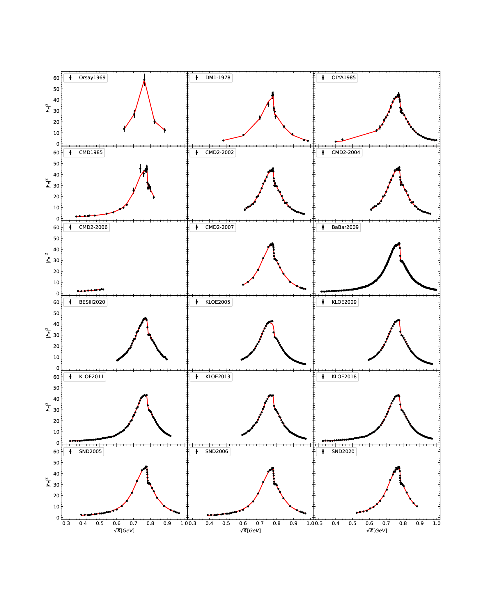
Furthermore, using the BW types of BW1, BW2, GS and KS models, one can also determine the parameters of $\rho$ meson, $M_{\rho}$ and $\Gamma_{\rho}$, from the fits, see the results of Table II. Note that in the first column, the ones for the HL model are not obtained directly from the fits. As discussed in Refs. Heyn:1980bh; Gardner:1997ie, once the parameters $a,\ b,\ c$ were determined from the fit, the $M_{\rho}$ and $\Gamma_{\rho}$ could also be determined, since the function $f(s)$, see Eq. (33), should be matched with the BW form when $s\to M_{\rho}^{2}$. And thus, one can have $\mathrm{Re}[f(M_{\rho}^{2})]=0$ and $\mathrm{Im}[f(M_{\rho}^{2})]=-M_{\rho}\Gamma_{\rho}$. Since the small uncertainties are obtained from the fits for the parameters of $a$, $b$, and $c$, the uncertainties for their results of determining $M_{\rho}$ and $\Gamma_{\rho}$ are small too, also for the results of $a_{\mu}^{\mathrm{HVP},\mathrm{LO}}$ later. For the data of CMD2-2006, because the data is close to the $\pi\pi$ threshold, it is not possible to get the results for $M_{\rho}$ and $\Gamma_{\rho}$ correctly. The results for Orsay1969 are bigger than the others, whereas the ones for KLOE2005 are much smaller. And compared with different models, the results with the BW2 model are bigger than the ones with the BW1 model, and also larger than the numbers obtained with the GS (or KS) model. Finally, we obtain the results of the $\rho$ meson parameters, $M_{\rho}$ and $\Gamma_{\rho}$ ⁴⁴ 4 In fact, these results are for the neutral one of $\rho^{0}$ meson in the $e^{+}e^{-}$ annihilation processes., from the fit with GS (or KS) model and the Com. Dat.,

$$M_{\rho}=(774.07\pm 0.04)\ \text{MeV},\quad\Gamma_{\rho}=(149.54\pm 0.08)\ \text{MeV},$$

(55)

which are 1 MeV smaller than the one reported in PDG Zyla:2020zbs, $(775.26\pm 0.23)$ MeV, for the mass, and 2 MeV bigger than the one $(147.4\pm 0.8)$ MeV for the width, and a bit smaller than the other one $M_{\rho}=(775.13\pm 0.02)$ MeV obtained in Ref. Pich:2001pj. Our results are also consistent with the one obtained in Ref. Davier:2019can, $M_{\rho}=(774.5\pm 0.8)$ MeV. Note that, the small errors for the pole parameters are due to more constraints in the Com. Dat.. One thing should be remarked that, as discussed above and shown in Table II, the $\rho$ meson parameters, $M_{\rho}$ and $\Gamma_{\rho}$, are model dependent and do not correspond to the physical resonance’s mass and width, which should be looked for the pole in the second Riemann sheet. It is complicated to extrapolate the form factor to the second Riemann sheet GBarton, which is out of our concern in the present work and where one can refer to Refs. Gonzalez-Solis:2019iod; GomezDumm:2013sib for more discussions ⁵⁵ 5 In their model, a pole $(762.0\pm 0.3,\frac{i}{2}(143.0\pm 0.2)\,)$ MeV was found for a mass parameter $M_{\rho}=(775.2\pm 0.4)$ MeV from the fitting of $\tau$ decay data. and Ref. LHCb:2021auc for the application in the unitarised three-body BW function.

Besides, for the other parameters, we show the results in Table IV in Appendix A, where the details for $\alpha$ and $\kappa$ are given and the results with Omnés model are consistent with the ones of Ref. Hanhart:2016pcd within the uncertainties. As done in Ref. Hanhart:2016pcd, one can extract the $\omega\pi\pi$ coupling and the branching ratio of $\omega\to\pi\pi$ from the results of $\kappa$ parameter in Table IV. Thus, following the same way and using the favoured results of GS (or KS) model for the Com. Dat., $\kappa=(1.77\pm 0.01)\times 10^{-3}$, we have

$$g_{\omega\pi\pi}=(3.02\pm 0.05)\times 10^{-2},\quad\text{Br}(\omega\to\pi\pi)=(1.52\pm 0.06)\%,$$

(56)

which are consistent with the ones obtained in Ref. Hanhart:2016pcd within the uncertainties. Our result for the branching ratio is also in good agreement with the one in PDG Zyla:2020zbs, $\text{Br}(\omega\to\pi\pi)=(1.53^{+0.11}_{-0.13})\%$.

References

- (1) R. L. Garwin, L. M. Lederman and M. Weinrich, Phys. Rev. 105, 1415-1417 (1957).
- (2) R. L. Garwin, D. P. Hutchinson, S. Penman and G. Shapiro, Phys. Rev. 118, 271-283 (1960).
- (3) H. Terazawa, Prog. Theor. Phys. 39, 1326-1332 (1968).
- (4) H. Terazawa, Prog. Theor. Phys. 40, 830-833 (1968).
- (5) H. Terazawa, Phys. Rev. 177, 2159-2166 (1969).
- (6) T. Kinoshita, J. Pestieau, P. Roy and H. Terazawa, Phys. Rev. D 2, 910-918 (1970).
- (7) H. Terazawa, Nonlin. Phenom. Complex Syst. 21, no.3, 268-272 (2018).
- (8) F. Jegerlehner and A. Nyffeler, Phys. Rept. 477, 1-110 (2009) [arXiv:0902.3360 [hep-ph]].
- (9) J. P. Miller, E. de Rafael, B. L. Roberts and D. Stöckinger, Ann. Rev. Nucl. Part. Sci. 62, 237-264 (2012).
- (10) G. W. Bennett et al. [Muon g-2], Phys. Rev. D 73, 072003 (2006) [arXiv:hep-ex/0602035 [hep-ex]].
- (11) P. J. Mohr, B. N. Taylor and D. B. Newell, Rev. Mod. Phys. 84, 1527-1605 (2012) [arXiv:1203.5425 [physics.atom-ph]].
- (12) M. Davier, A. Hoecker, B. Malaescu and Z. Zhang, Eur. Phys. J. C 80, no.3, 241 (2020) [erratum: Eur. Phys. J. C 80, no.5, 410 (2020)] [arXiv:1908.00921 [hep-ph]].
- (13) B. Abi et al. [Muon g-2], Phys. Rev. Lett. 126, no.14, 141801 (2021) [arXiv:2104.03281 [hep-ex]].
- (14) T. Aoyama, N. Asmussen, M. Benayoun, J. Bijnens, T. Blum, M. Bruno, I. Caprini, C. M. Carloni Calame, M. Cè and G. Colangelo, et al. Phys. Rept. 887, 1-166 (2020) [arXiv:2006.04822 [hep-ph]].
- (15) C. W. Chiang and K. Yagyu, Phys. Rev. D 103, no.11, L111302 (2021) [arXiv:2104.00890 [hep-ph]].
- (16) A. E. Cárcamo Hernández, C. Espinoza, J. Carlos Gómez-Izquierdo and M. Mondragón, [arXiv:2104.02730 [hep-ph]].
- (17) G. Arcadi, L. Calibbi, M. Fedele and F. Mescia, [arXiv:2104.03228 [hep-ph]].
- (18) B. Zhu and X. Liu, [arXiv:2104.03238 [hep-ph]].
- (19) M. Endo, K. Hamaguchi, S. Iwamoto and T. Kitahara, [arXiv:2104.03217 [hep-ph]].
- (20) X. F. Han, T. Li, H. X. Wang, L. Wang and Y. Zhang, [arXiv:2104.03227 [hep-ph]].
- (21) P. Das, M. K. Das and N. Khan, [arXiv:2104.03271 [hep-ph]].
- (22) S. F. Ge, X. D. Ma and P. Pasquini, [arXiv:2104.03276 [hep-ph]].
- (23) S. Baum, M. Carena, N. R. Shah and C. E. M. Wagner, [arXiv:2104.03302 [hep-ph]].
- (24) H. B. Zhang, C. X. Liu, J. L. Yang and T. F. Feng, [arXiv:2104.03489 [hep-ph]].
- (25) W. Ahmed, I. Khan, J. Li, T. Li, S. Raza and W. Zhang, [arXiv:2104.03491 [hep-ph]].
- (26) J. Cao, J. Lian, Y. Pan, D. Zhang and P. Zhu, [arXiv:2104.03284 [hep-ph]].
- (27) A. Crivellin and M. Hoferichter, JHEP 07, 135 (2021) [arXiv:2104.03202 [hep-ph]].
- (28) P. Athron, C. Balázs, D. H. Jacob, W. Kotlarski, D. Stöckinger and H. Stöckinger-Kim, [arXiv:2104.03691 [hep-ph]].
- (29) W. Yin and M. Yamaguchi, [arXiv:2012.03928 [hep-ph]].
- (30) W. Yin and W. Yin, [arXiv:2103.14234 [hep-ph]].
- (31) W. Yin, JHEP 06, 029 (2021) [arXiv:2104.03259 [hep-ph]].
- (32) H. Terazawa, Quark Matter: From Subquarks to the Universe, Physics Research and Technology, Nov. 2018, NOVA.
- (33) A. Keshavarzi, K. S. Khaw and T. Yoshioka, [arXiv:2106.06723 [hep-ex]].
- (34) P. A. Zyla et al. [Particle Data Group], PTEP 2020, no.8, 083C01 (2020).
- (35) T. Aoyama, M. Hayakawa, T. Kinoshita and M. Nio, Phys. Rev. Lett. 109, 111807 (2012) [arXiv:1205.5368 [hep-ph]].
- (36) T. Aoyama, M. Hayakawa, T. Kinoshita and M. Nio, Phys. Rev. Lett. 109, 111808 (2012) [arXiv:1205.5370 [hep-ph]].
- (37) P. A. Baikov, A. Maier and P. Marquard, Nucl. Phys. B 877, 647-661 (2013) [arXiv:1307.6105 [hep-ph]].
- (38) S. Volkov, Phys. Rev. D 100, no.9, 096004 (2019) [arXiv:1909.08015 [hep-ph]].
- (39) A. Czarnecki, W. J. Marciano and A. Vainshtein, Phys. Rev. D 67, 073006 (2003) [erratum: Phys. Rev. D 73, 119901 (2006)] [arXiv:hep-ph/0212229 [hep-ph]].
- (40) C. Gnendiger, D. Stöckinger and H. Stöckinger-Kim, Phys. Rev. D 88, 053005 (2013) [arXiv:1306.5546 [hep-ph]].
- (41) T. Ishikawa, N. Nakazawa and Y. Yasui, Phys. Rev. D 99, no.7, 073004 (2019) [arXiv:1810.13445 [hep-ph]].
- (42) K. Melnikov and A. Vainshtein, Phys. Rev. D 70, 113006 (2004) [arXiv:hep-ph/0312226 [hep-ph]].
- (43) P. Masjuan and P. Sánchez-Puertas, Phys. Rev. D 95, no.5, 054026 (2017) [arXiv:1701.05829 [hep-ph]].
- (44) G. Colangelo, M. Hoferichter, M. Procura and P. Stoffer, JHEP 04, 161 (2017) [arXiv:1702.07347 [hep-ph]].
- (45) M. Hoferichter, B. L. Hoid, B. Kubis, S. Leupold and S. P. Schneider, JHEP 10, 141 (2018) [arXiv:1808.04823 [hep-ph]].
- (46) A. Gérardin, H. B. Meyer and A. Nyffeler, Phys. Rev. D 100, no.3, 034520 (2019) [arXiv:1903.09471 [hep-lat]].
- (47) J. Bijnens, N. Hermansson-Truedsson and A. Rodríguez-Sánchez, Phys. Lett. B 798, 134994 (2019) [arXiv:1908.03331 [hep-ph]].
- (48) T. Blum, N. Christ, M. Hayakawa, T. Izubuchi, L. Jin, C. Jung and C. Lehner, Phys. Rev. Lett. 124, no.13, 132002 (2020) [arXiv:1911.08123 [hep-lat]].
- (49) E. H. Chao, R. J. Hudspith, A. Gérardin, J. R. Green, H. B. Meyer and K. Ottnad, [arXiv:2104.02632 [hep-lat]].
- (50) J. Lüdtke and M. Procura, Eur. Phys. J. C 80, no.12, 1108 (2020) [arXiv:2006.00007 [hep-ph]].
- (51) J. Bijnens, N. Hermansson-Truedsson, L. Laub and A. Rodríguez-Sánchez, JHEP 10, 203 (2020) [arXiv:2008.13487 [hep-ph]].
- (52) J. Bijnens, N. Hermansson-Truedsson, L. Laub and A. Rodríguez-Sánchez, JHEP 04, 240 (2021) [arXiv:2101.09169 [hep-ph]].
- (53) P. Masjuan, P. Roig and P. Sanchez-Puertas, [arXiv:2005.11761 [hep-ph]].
- (54) P. Roig and P. Sanchez-Puertas, Phys. Rev. D 101, no.7, 074019 (2020) [arXiv:1910.02881 [hep-ph]].
- (55) L. Cappiello, O. Catà, G. D’Ambrosio, D. Greynat and A. Iyer, Phys. Rev. D 102, no.1, 016009 (2020) [arXiv:1912.02779 [hep-ph]].
- (56) M. Zanke, M. Hoferichter and B. Kubis, [arXiv:2103.09829 [hep-ph]].
- (57) J. Leutgeb and A. Rebhan, Phys. Rev. D 101, no.11, 114015 (2020) [arXiv:1912.01596 [hep-ph]].
- (58) I. Danilkin, M. Hoferichter and P. Stoffer, [arXiv:2105.01666 [hep-ph]].
- (59) G. Colangelo, F. Hagelstein, M. Hoferichter, L. Laub and P. Stoffer, Eur. Phys. J. C 81, no.8, 702 (2021) [arXiv:2106.13222 [hep-ph]].
- (60) A. Keshavarzi, D. Nomura and T. Teubner, Phys. Rev. D 101, no.1, 014029 (2020) [arXiv:1911.00367 [hep-ph]].
- (61) A. Kurz, T. Liu, P. Marquard and M. Steinhauser, Phys. Lett. B 734, 144-147 (2014) [arXiv:1403.6400 [hep-ph]].
- (62) M. Davier, A. Hoecker, B. Malaescu and Z. Zhang, Eur. Phys. J. C 77, no.12, 827 (2017) [arXiv:1706.09436 [hep-ph]].
- (63) A. Keshavarzi, D. Nomura and T. Teubner, Phys. Rev. D 97, no.11, 114025 (2018) [arXiv:1802.02995 [hep-ph]].
- (64) G. Colangelo, M. Hoferichter and P. Stoffer, JHEP 02, 006 (2019) [arXiv:1810.00007 [hep-ph]].
- (65) M. Hoferichter, B. L. Hoid and B. Kubis, JHEP 08, 137 (2019) [arXiv:1907.01556 [hep-ph]].
- (66) S. Borsanyi, Z. Fodor, J. N. Guenther, C. Hoelbling, S. D. Katz, L. Lellouch, T. Lippert, K. Miura, L. Parato and K. K. Szabo, et al. Nature 593, no.7857, 51-55 (2021) [arXiv:2002.12347 [hep-lat]].
- (67) C. Lehner and A. S. Meyer, Phys. Rev. D 101, 074515 (2020) [arXiv:2003.04177 [hep-lat]].
- (68) M. Davier, A. Höcker, B. Malaescu, C. Z. Yuan and Z. Zhang, Eur. Phys. J. C 74, no.3, 2803 (2014) [arXiv:1312.1501 [hep-ex]].
- (69) S. Gonzàlez-Solís and P. Roig, Eur. Phys. J. C 79, no.5, 436 (2019) [arXiv:1902.02273 [hep-ph]].
- (70) J. A. Miranda and P. Roig, Phys. Rev. D 102, 114017 (2020) [arXiv:2007.11019 [hep-ph]].
- (71) M. Benayoun, L. Delbuono and F. Jegerlehner, Eur. Phys. J. C 80, no.2, 81 (2020) [erratum: Eur. Phys. J. C 80, no.3, 244 (2020)] [arXiv:1903.11034 [hep-ph]].
- (72) M. Benayoun, L. DelBuono and F. Jegerlehner, [arXiv:2105.13018 [hep-ph]].
- (73) H. n. Li and H. Umeeda, Phys. Rev. D 102, no.9, 094003 (2020) [arXiv:2004.06451 [hep-ph]].
- (74) C. Aubin, T. Blum, M. Golterman and S. Peris, Phys. Rev. D 102, no.9, 094511 (2020) [arXiv:2008.03809 [hep-lat]].
- (75) B. Malaescu and M. Schott, Eur. Phys. J. C 81, no.1, 46 (2021) [arXiv:2008.08107 [hep-ph]].
- (76) A. Crivellin, M. Hoferichter, C. A. Manzari and M. Montull, Phys. Rev. Lett. 125, no.9, 091801 (2020) [arXiv:2003.04886 [hep-ph]].
- (77) M. Benayoun, P. David, L. DelBuono and F. Jegerlehner, Eur. Phys. J. C 75, no.12, 613 (2015) [arXiv:1507.02943 [hep-ph]].
- (78) G. Colangelo, M. Hoferichter and P. Stoffer, Phys. Lett. B 814, 136073 (2021) [arXiv:2010.07943 [hep-ph]].
- (79) B. Ananthanarayan, I. Caprini, D. Das and I. Sentitemsu Imsong, Phys. Rev. D 93, no.11, 116007 (2016) [arXiv:1605.00202 [hep-ph]].
- (80) B. Ananthanarayan, I. Caprini and D. Das, Phys. Rev. D 98, no.11, 114015 (2018) [arXiv:1810.09265 [hep-ph]].
- (81) B. Ananthanarayan, I. Caprini and D. Das, Phys. Rev. D 102, no.9, 096003 (2020) [arXiv:2008.00669 [hep-ph]].
- (82) M. Gourdin and E. De Rafael, Nucl. Phys. B 10, 667-674 (1969).
- (83) M. Roos, Nucl. Phys. B 97, 165-177 (1975)
- (84) C. B. Lang and I. S. Stefanescu, Phys. Lett. B 58, 450-454 (1975).
- (85) R. Omnés, Nuovo Cim. 8, 316-326 (1958)
- (86) A. Pich and J. Portoles, Phys. Rev. D 63, 093005 (2001) [arXiv:hep-ph/0101194 [hep-ph]].
- (87) M. Hoferichter, B. Kubis, S. Leupold, F. Niecknig and S. P. Schneider, Eur. Phys. J. C 74, 3180 (2014) [arXiv:1410.4691 [hep-ph]].
- (88) T. Isken, B. Kubis, S. P. Schneider and P. Stoffer, Eur. Phys. J. C 77, no.7, 489 (2017) [arXiv:1705.04339 [hep-ph]].
- (89) F. Stollenwerk, C. Hanhart, A. Kupsc, U. G. Meissner and A. Wirzba, Phys. Lett. B 707, 184-190 (2012) [arXiv:1108.2419 [nucl-th]].
- (90) C. Hanhart, A. Kupśc, U.-G. Meißner, F. Stollenwerk and A. Wirzba, Eur. Phys. J. C 73, no.12, 2668 (2013) [erratum: Eur. Phys. J. C 75, no.6, 242 (2015)] [arXiv:1307.5654 [hep-ph]].
- (91) C. Hanhart, Phys. Lett. B 715, 170-177 (2012) [arXiv:1203.6839 [hep-ph]].
- (92) R. Garcia-Martin, R. Kaminski, J. R. Pelaez, J. Ruiz de Elvira and F. J. Yndurain, Phys. Rev. D 83, 074004 (2011) [arXiv:1102.2183 [hep-ph]].
- (93) N. N. Achasov and A. A. Kozhevnikov, JETP Lett. 96, 559-563 (2013) [arXiv:1209.5524 [hep-ph]].
- (94) N. N. Achasov and A. A. Kozhevnikov, Phys. Rev. D 88, no.9, 093002 (2013) [arXiv:1305.6117 [hep-ph]].
- (95) I. V. Danilkin, C. Fernández-Ramírez, P. Guo, V. Mathieu, D. Schott, M. Shi and A. P. Szczepaniak, Phys. Rev. D 91, no.9, 094029 (2015) [arXiv:1409.7708 [hep-ph]].
- (96) M. F. Heyn and C. B. Lang, Z. Phys. C 7, 169-181 (1981).
- (97) G. J. Gounaris and J. J. Sakurai, Phys. Rev. Lett. 21, 244-247 (1968).
- (98) J. P. Lees et al. [BaBar], Phys. Rev. D 86, 032013 (2012) [arXiv:1205.2228 [hep-ex]].
- (99) J. H. Kühn and A. Santamaria, Z. Phys. C 48, 445-452 (1990).
- (100) C. Hanhart, S. Holz, B. Kubis, A. Kupść, A. Wirzba and C. W. Xiao, Eur. Phys. J. C 77, no.2, 98 (2017) [arXiv:1611.09359 [hep-ph]].
- (101) H. B. O’Connell, B. C. Pearce, A. W. Thomas and A. G. Williams, Prog. Part. Nucl. Phys. 39, 201-252 (1997) [arXiv:hep-ph/9501251 [hep-ph]].
- (102) J. E. Augustin, J. C. Bizot, J. Buon, J. Haissinski, D. Lalanne, P. Marin, H. Nguyen Ngoc, J. Perez-Y-Jorba, F. Rumpf, E. Silva and S. Tavernier, Phys. Lett. B 28, 508-512 (1969)
- (103) A. Quenzer, M. Ribes, F. Rumpf, J. L. Bertrand, J. C. Bizot, R. L. Chase, A. Cordier, B. Delcourt, P. Eschstruth, F. Fulda, G. Grosdidier, J. Haissinski, J. Jeanjean, M. Jeanjean, R. J. Madaras, J. L. Masnou and J. Perez-Y-Jorba, Phys. Lett. B 76, 512-516 (1978)
- (104) L. M. Barkov, A. G. Chilingarov, S. I. Eidelman, B. I. Khazin, M. Y. Lelchuk, V. S. Okhapkin, E. V. Pakhtusova, S. I. Redin, N. M. Ryskulov, Y. M. Shatunov, A. I. Shekhtman, B. A. Shvarts, V. A. Sidorov, A. N. Skrinsky, V. P. Smakhtin and E. P. Solodov, Nucl. Phys. B 256, 365-384 (1985)
- (105) R. R. Akhmetshin et al. [CMD-2], Phys. Lett. B 527, 161-172 (2002) [arXiv:hep-ex/0112031 [hep-ex]].
- (106) R. R. Akhmetshin et al. [CMD-2], Phys. Lett. B 578, 285-289 (2004) [arXiv:hep-ex/0308008 [hep-ex]].
- (107) V. M. Aul’chenko et al. [CMD-2], JETP Lett. 82, 743-747 (2005) [arXiv:hep-ex/0603021 [hep-ex]].
- (108) V. M. Aul’chenko et al., JETP Lett. 84, 413-417 (2006) [arXiv:hep-ex/0610016 [hep-ex]].
- (109) R. R. Akhmetshin et al. [CMD-2], Phys. Lett. B 648, 28-38 (2007) [arXiv:hep-ex/0610021 [hep-ex]].
- (110) B. Aubert et al. [BaBar], Phys. Rev. Lett. 103, 231801 (2009) [arXiv:0908.3589 [hep-ex]].
- (111) M. Ablikim et al. [BESIII], Phys. Lett. B 753, 629-638 (2016) [arXiv:1507.08188 [hep-ex]].
- (112) M. Ablikim et al. [BESIII], [arXiv:2009.05011 [hep-ex]].
- (113) A. Aloisio et al. [KLOE], Phys. Lett. B 606, 12-24 (2005) [arXiv:hep-ex/0407048 [hep-ex]].
- (114) F. Ambrosino et al. [KLOE], Phys. Lett. B 670, 285-291 (2009) [arXiv:0809.3950 [hep-ex]].
- (115) F. Ambrosino et al. [KLOE], Phys. Lett. B 700, 102-110 (2011) [arXiv:1006.5313 [hep-ex]].
- (116) D. Babusci et al. [KLOE], Phys. Lett. B 720, 336-343 (2013) [arXiv:1212.4524 [hep-ex]].
- (117) A. Anastasi et al. [KLOE-2], JHEP 03, 173 (2018) [arXiv:1711.03085 [hep-ex]].
- (118) M. N. Achasov et al., J. Exp. Theor. Phys. 101, no.6, 1053-1070 (2005) [arXiv:hep-ex/0506076 [hep-ex]].
- (119) M. N. Achasov et al., J. Exp. Theor. Phys. 103, 380-384 (2006) [arXiv:hep-ex/0605013 [hep-ex]].
- (120) M. N. Achasov et al. [SND], [arXiv:2004.00263 [hep-ex]].
- (121) S. Gardner and H. B. O’Connell, Phys. Rev. D 57, 2716-2726 (1998) [erratum: Phys. Rev. D 62, 019903 (2000)] [arXiv:hep-ph/9707385 [hep-ph]].
- (122) G. Barton, “Introduction to Dispersion techniques in field theory,” W.A. Benjamin, Inc. 1965, New York.
- (123) D. Gómez Dumm and P. Roig, Eur. Phys. J. C 73, no.8, 2528 (2013) [arXiv:1301.6973 [hep-ph]].
- (124) R. Aaij et al. [LHCb], [arXiv:2109.01056 [hep-ex]].
- (125) W. Qin, L. Y. Dai and J. Portolés, JHEP 03, 092 (2021) [arXiv:2011.09618 [hep-ph]].