BICNet: A Bayesian Approach for Estimating Task Effects
on Intrinsic Connectivity Networks in fMRI Data
Abstract
Intrinsic connectivity networks (ICNs) are specific dynamic functional brain networks that are consistently found under various conditions including rest and task. Studies have shown that some stimuli actually activate intrinsic connectivity through either suppression, excitation, moderation or modification. Nevertheless, the structure of ICNs and task-related effects on ICNs are not yet fully understood. In this paper, we propose a Bayesian Intrinsic Connectivity Network (BICNet) model to identify the ICNs and quantify the task-related effects on the ICN dynamics. Using an extended Bayesian dynamic sparse latent factor model, the proposed BICNet has the following advantages: (1) it simultaneously identifies the individual ICNs and group-level ICN spatial maps; (2) it robustly identifies ICNs by jointly modeling resting-state functional magnetic resonance imaging (rfMRI) and task-related functional magnetic resonance imaging (tfMRI); (3) compared to independent component analysis (ICA)-based methods, it can quantify the difference of ICNs amplitudes across different states; (4) it automatically performs feature selection through the sparsity of the ICNs rather than ad-hoc thresholding. The proposed BICNet was applied to the rfMRI and language tfMRI data from the Human Connectome Project (HCP) and the analysis identified several ICNs related to distinct language processing functions.
Keywords:
fMRI , Intrinsic Connectivity , Dynamic Functional Connectivity , Bayesian Hierarchical Model , Latent Factor1 Introduction
Functional brain networks are dynamically evolving to satisfy our ongoing demands, resulting from either external stimuli or internal processes. However, many studies have reported high spatial similarity and relatively low spatial dissimilarity between dynamic functional brain networks under resting and task-related states [1, 2, 3]. Also, some studies observe some networks consistently presenting across populations, including both healthy subjects and patients. It indicates that there is an intrinsic connectivity network (ICN) that persists under various cognitive conditions and across a population. These observations suggest that dynamic functional brain networks consist of both on-demand dynamics and intrinsic dynamics that support the fundamental brain functions. Recent research demonstrates that intrinsic connectivity correlates with cognition and behavioral performance [4]. Some studies show evidence of alterations in ICN in patients with neurological disorders, e.g., Alzheimer’s disease, epilepsy, and schizophrenia, relative to the healthy control population. These findings strongly indicate that intrinsic connectivity can be a biomarker of neurological disorders [5, 4, 6, 7].
This paper aims to identify dynamic ICNs at the individual level and the corresponding intrinsic spatial maps at the group level using the proposed Bayesian Intrinsic Connectivity Network (BICNet) model. Moreover, we aim to develop a formal statistical framework under which neuroscientists can compare the dynamics of different ICNs under different cognitive conditions, such as resting vs. task-related states. Note that we use connectivity and network interchangeably in this paper.
The key question is how to define the concept of ICN. Early studies consider resting-state connectivity networks as ICNs [8, 9, 10]. However, resting-state ICNs are confounded by unconscious context [11] and hard to be related to certain cognitive functions. In the proposed BICNet model, we pool the information from both rfMRI and tfMRI together to improve robustness and interpretability. Then the question turns into in what form ICN exists in the dynamic functional networks under resting and task-related states. We adopt an intuitive assumption that some brain regions are intrinsically linked to networks with specialized roles in information processing. Then, a cognitive task dynamically engages multiple intrinsic networks [12]. In other words, ICNs are considered as unobservable components of dynamic functional networks that have relatively stable spatial structures but dynamic activities. The stimuli can activate ICNs through either suppression, excitation, moderation, or modification. This definition can be naturally translated into a latent factor model, . We measure the dynamic functional connectivity by dynamic correlation, which can be estimated by BICNet. Studying dynamic correlation is equivalent to study the dynamic variance, .
Further, we can see that captures all the network dynamics, and thus we define as the amplitudes of ICNs, which captures the dynamics of ICN activations. Here we adopt the concept of stochastic volatility from economics. Volatility indeed is the variance of a time series, which is also considered a time-dependent random variable [13, 14]. For example, in the stock market prices, we can observe that large changes tend to cluster together [15], which tells us that the variance of the stock market prices is time-dependent. The stochastic model assumes that the alternation of volatile and tranquil periods is governed by unobservable information flows that are internally generated and never extinguished [16]. This intuition provides a conceptual similarity between financial market fluctuations and brain activities. It is natural to consider that some intrinsic neuronal processes dominate hemodynamic activity measured by functional magnetic resonance imaging (fMRI). These intrinsic neuronal processes are continuously evolving and can become volatile while excited or inhibited by external stimuli or internal demands. Neuroscientists suggest that human brain networks and financial market networks have a certain degree of topological isomorphism [17]. Both of these networks have intrinsic properties and respond to external shocks to the system.
Even though ICA is a very popular method in ICN studies, it imposes a restriction to solve the non-identifiability issue [18]. Therefore, it only produces spatial maps but not dynamic networks. On the contrary, BICNet imposes identifiability restriction on which captures the spatial structure of ICNs but maintain the flexibility of modeling dynamic ICN amplitudes. There are limited attempts to go beyond ICA and study the dynamic ICNs. [19] proposes a statistical framework using Bayesian Gaussian graphical model with a restricted assumption of temporal dependence of fMRI signals. Thus, there is a need to develop a rigorous statistical model to capture the dynamic nature of connectivity and provide a platform for testing the difference between ICNs under various conditions, such as across patient groups, across various types of cognitive tasks.
In a recent paper, [20] discusses methods for change point detection of brain states and a general latent model, which assumes unknown sources and unknown time-varying membership. In contrast, the proposed BICNet model focuses on identifying ICNs with fixed membership and time-varying amplitudes.
Here, we highlight the main difference between the proposed BICNet from the ICA-based methods: (1) BICNet can estimate the amplitudes of ICNs. (2) Existing methods for identifying ICNs for fMRI such as ICA essentially produce co-activation networks (i.e., sets of distributed co-activated brain regions); in contrast, BICNet can estimate both the co-activation patterns and the strength of connectivity between regions. (3) The sparsity of ICNs automatically performs feature selection, instead of ad-hoc thresholding.
The contributions of our proposed BICNet model are the following: (1) Its hierarchical structure can simultaneously capture group-level and individual-level variations in ICNs in a more flexible way. (2) It can quantify the difference of ICNs amplitudes across different states under a natural statistical inference framework; (3) It identifies multiple ICNs in a latent subspace, which enables neuroscientists to test for associations between ICNs with various behavioral measures. (4) It jointly models rfMRI and tfMRI which can produce behaviorally meaningful ICNs.
The paper is organized as follows. Section 2 introduces the BICNet model, including the model specification, MCMC estimation, and inference. Section 3 contains results from extensive simulation studies that investigated the shrinkage behavior of the spike-and-slab prior, the performance of BICNet compared with group ICA algorithm. In Section 4, the proposed model is utilized to analyze the rfMRI and tfMRI data sets from the HCP. We conclude with a summary and some future extensions of BICNet in Section 5.
2 Methodology: BICNet
2.1 Modeling Dynamic Functional Connectivity by Low-Rank Representation
To begin with, the modeling of dynamic functional connectivity is based on a widely used generalized linear model at voxel level for fMRI studies, , where denotes the original fMRI signal observed at time , captures the hemodynamic responses, and captures functional connectivity in its second or higher order moments. Further, we regress out the activation, , since our primary interest is the functional connectivity pattern captured by . Optionally, we can group the voxels in into a region of interest (ROI) in using a pre-defined atlas to ease the computation burden. We define as the -variate fMRI signals of subject under experimental condition with the deterministic mean structure removed. Specifically, refers to the resting state. Therefore, reflects the intrinsic neuronal processes in the lack of external stimuli, and , , contains information about the alteration of these intrinsic processes evoked by external stimuli.
In the remaining part of this session, we focus on of an individual at a given experimental condition , and drop and for simplicity. We model the random component with a conditional Gaussian distribution with time-varying variance , i.e., , . Using a latent factor model, we project into a lower dimensional subspace, , where the latent process , , is the isotropic residual with , and is the factor loading matrix that captures the time-invariant spatial ICN structures. It is equivalent to decompose the variance-covariance matrix by . Further, we define as the th column vector of , and thus . Also, we assume the latent processes are uncorrelated and thus .

Specifically, the denoised dynamic functional connectivity is defined as =. As shown in fig. 1, this denoised whole-brain functional connectivity can be decomposed into ICNs with changing dynamics of their corresponding amplitudes. We define ICN as , where is the dynamic amplitude of ICN , and captures the spatial structure or the co-activation pattern of ICN , that is, the membership of ICN and the contribution of each ROI that belongs to this ICN. From another perspective, ICN is an undirected graph where defines a set of vertices and their corresponding weights, defines the edges between vertices, and controls the overall weights of edges.
2.2 Modeling the Structure of ICN by Sparse Hierarchical Model
In this section, we model both individual ICNs and the corresponding group-level spatial maps. We add subscript to indicate a subject but drop the superscript since the ICN structure is invariant across different experimental conditions.
As previously mentioned, the ICN structure , , consists of membership and the contribution of each member in this ICN. The zero-nonzero patterns, represent the membership of the -th ICN. A real non-zero value, , represents the contribution of a ROI to an ICN . While the ICN memberships can overlap with each other, the dynamics of the -th ICN are uncorrelated to other ICNs’ dynamics, given that is a diagonal matrix. Note here that ICNs are defined in the latent subspace instead of the whole-brain ROI space.

The structure of an ICN is time-invariant and task-invariant. Mathematically, this assumption is necessary to ensure the identifiability of the connectivity parameters. Biologically, this assumption indicates that the structure of every ICN component is subject-specific and relatively stable across time. However, the BICNet model enables dynamic modifications on the amplitudes of ICN components, which can capture a wide range of global ICN structures. As shown in the second column of fig. 2, the structure of ICN 1 remains the same while the amplitude changes from time to . The changes in the amplitudes of the ICN components can lead to a reconfiguration of the whole-brain functional connectivity networks, as shown in the last column of fig. 2. Furthermore, this specification is consistent with many studies that suggest that the ICN structures are relatively stable across conditions. Finally, this model does not constrain the intrinsic connectivity network, , to be constant in time because the state-specific factor variance matrix is allowed to change over time. Therefore, the advantage of BICNet is its ability to capture the dynamic nature of brain connectivity.
In the proposed model, the structure of ICNs, , is sparse in the sense that a specific region is a member of some ICNs, and an ICN only includes a subset of regions. To achieve sparsity, we use the standard spike-and-slab prior [21, 22] consisting of a Dirac “spike” component that puts a probability mass at zero, and a normal “slab” component has its mass spread over a wide range of possible values, as shown in eq. 1.
| (1) | ||||
| (2) | ||||
| (3) |
where denotes that region is included in the -th ICN for subject , while indicates otherwise. We assume , , which means that the probability of inclusion of region in the -th ICN is denoted to be .
The model currently assumes that is constant across subjects and call it group inclusion probability at . Here, “group” refers to the group of all the subjects. The group inclusion probability matrix, , captures the group-level probabilistic spatial maps. As shown in eq. 3, a beta distribution is utilized to express our uncertainty about this group inclusion probability. The prior expectation of is . With this setting, neuroscientists can use biological or experimental information by setting as well-known ICN templates, ICA spatial maps, or principal component analysis (PCA) results. Otherwise, a non-informative uniform prior, is used.
The spike-and-slab prior represents the relationship between individual ICN and the group-level spatial map . The ICN ’s structure of subject has the same mathematical meaning as the ICN ’s structure of subject , , since they are all derived from the group-level spatial map . Note that while the probability is common across all subjects, it can flexibly adapt to variations across subjects. The variation in individual ICN membership is captured by the indicator , and the variation in the contribution of ROI to ICN is captured by .
2.3 Modeling the Amplitude of ICN by Factor Stochastic Volatility
We consider a dynamic functional brain network as a mixture of ICNs that can be either tranquil or volatile. It is natural to assume that when a specific ICN is activated, either excited or inhibited, its amplitude will first be more volatile than the baseline level and then gradually returns to the baseline level. Specifically, when an ICN is excited or inhibited, the amplitude, measured by , either increases or decreases. We consider both excitation and suppression as activation. Inactivation is defined as no significant change in amplitudes compared to those in the resting state. The dynamics of ICN amplitudes can be model by the factor stochastic volatility model in eq. 4, which is proposed by [23].
| (4) | ||||
where , , , , and .
The autoregressive (AR) (1) process is used to model the dynamics of variance at the logarithm scale, capable of capturing realistic hidden brain states that are nonlinear and continuous. Due to the short length of fMRI time series, it is common to use AR (1) rather than higher-order ARs and these are often known to sufficiently capture the temporal structure [24, 25, 22].
2.4 Modeling the Behavioral Responses by Sparse Linear Regression
One of the main interests in neuroscience studies is to identify behaviorally meaningful specific ICN components. Our proposed approach allows associations between subject-specific changes of amplitudes of certain ICN components and behavioral response under experimental condition which is denoted by . These behavioral responses include accuracy, response time, or difficulty level of a specific task.
As shown in eq. 4, the expected amplitude of latent component under a specific condition for a single subject is captured by . If the true values of is known, then the effect of a task-related stimulus on a single latent factor can be quantified by the degree of deviation of , , from . Since the true values are not known, the deviation between the posterior distributions of , and is measured using the two-sided two-sample Kolmogorov-Smirnov (KS) test statistic, denoted by , . The KS statistic is a valid metric because it is symmetric, positive valued (it lies in the unit interval ), and satisfies the triangle inequality. A large value of indicates ICN of subject is activated. To further distinguish inhibition and excitation under activation, we calculate the sign of the difference between the posterior means, , with . Thus, a small value of indicates no activation, whereas a large value of with indicates inhibition, and a large value of with indicates excitation.
A regression model is employed to investigate the association between behavioral measures, and the changes of amplitudes of the ICNs during task performance relative to the resting state, measured by :
| (5) |
where the regression coefficient measures the contribution of each ICNs ‘’ change of amplitudes to the behavioral response, is the variance of the behavioral measure. The variance parameter follows an inverse Gamma distribution, . For , we assume that only a few of ICNs have contribution to , thus we use a spike-and-slab prior on .
| (6) | ||||
| (7) |
For a behavioral response , if the 95% credible interval of ’s posterior distribution does not contain zero, we say that there is an association between the -th ICN component and this behavioral response at the group level. From this model, one can identify the ICNs whose differential effect (task vs. rest) was significantly associated with accuracy, response time, story difficulty level, and math difficulty level, respectively.
2.5 Prior Distributions
For the univariate stochastic volatility (SV) processes, the prior distributions proposed by [23] will be used, i.e., , , and . Here, the Gamma distribution for is used instead of the conditionally conjugate inverse Gamma prior. Though the conjugate inverse Gamma prior is more commonly used because of computational efficiency, it bounds the variance away from zero a priori, leading to over-fitting in the state-space model [26, 27, 23]. The Gamma distribution for variance is equivalent to a truncated normal distribution for the standard deviation. There is some evidence suggesting that a Gaussian distribution [28] can reasonably approximate the rfMRI process. Therefore this choice prefers the simple normal distribution to the stochastic volatility process and is data-adaptive.
Conversely, the conjugate inverse Gamma is used for the regional-specific variance of the observed signals, , where is the shape parameter and is the rate parameter. Since fMRI data tends to have relatively small activation fluctuation compared with its noisy background [29], it is expected that the regional-specific white noise to account for a large part of the variation. Hence, the factor stochastic volatility process has a relatively small variation but contains more information about the hidden brain states. For behavioral responses, , which is the probability of having nonzero regression coefficients, is modeled as , and .
2.6 Estimation via MCMC
A Gibbs sampler augmented by some Metropolis-Hasting steps is constructed for factor stochastic volatility for our proposed model. The directed acyclic graph (DAG) is illustrated in fig. 3. The sampling process can be parallelized within each MCMC iterations because many conditional posterior distributions are independent of others. The factor loading matrix signs are not identifiable, and we solve this issue by post-processing after MCMC sampling. The sampling process is summarized as follows.
- 1.
We first update the regional-specific variances of the observed signals. Conditional on the latent factor structure, the observed signals follow a normal distribution, . Given the inverse Gamma prior, the conjugate conditional posterior distribution is . The sampling can be parallelized across and since they are conditionally independent.
- 2.
Sample stochastic volatilities of the latent factors, , and the corresponding parameters separately for every and using the 2-step MH sampler with centered parameterization and interweaved by a non-centered parameterization [30].
- 3.
For the sparse factor loadings, we first sample the sparse indicator based on its conditional posterior odds. If , then sample from its conjugate conditional posterior distribution, ; otherwise, set .
- 4.
Sample latent factor using a normal Bayesian regression update.
- 5.
Sample inclusion probability, or the group ICNs, using conditional posterior distribution: .
For the sparse linear regression of behavioral measures, we construct a Gibbs sampler as follows.
- 1.
We first update the probability of having nonzero regression coefficients with
- 2.
Then we sample .
- 3.
For the variance of behavioral measure , we have
- 4.
For the regression coefficient , which measures the contribution of ICNs, we have , where .
- 5.
Define . For , which indicates if , we have
2.7 Inference
BICNet can identify individual ICNs and group-level spatial maps. However, the group-level probability spatial maps, , are non-sparse inclusion probability matrices, while the individual ICNs are sparse matrices. We threshold at a selected probability value to aid the group-level interpretation. Similarly, in the following sections, we will estimate group ICA at the ROI-level using the Group ICA Of fMRI Toolbox (GIFT) algorithm. For the ICA spatial maps, we calculate the z-scores and threshold them at a selected value.
Identify ICNs and spatial maps that are related to language processing is equivalent to investigate the association between behavioral measures and the extent of activation (either suppression or excitation) of the ICNs during task performance relative to the resting state. We fit a linear regression model with behavioral measures as the dependent variables and the matrix as regressors. From the model, one can identify the ICNs whose differential effect (task vs. rest) was significantly associated with accuracy, response time, story difficulty level, and math difficulty level.
3 Simulation
3.1 Shrinkage Effect on ICNs with Different Underlying Sparsity
In the first experiment, the test is on inferring ICN structures under different sparsity levels. In other words, this experiment investigates the shrinkage effect of the spike-and-slab prior and how well it adapts to different levels of underlying sparsity on . We simulate a small-scale brain network of ROIs with latent ICNs with different levels of sparsity, as illustrated in fig. 4(a). To control the underlying sparsity, each subject has different ICN membership and the proportion of nonzero loadings in the factor loading matrix varies from 50% to 100%, with an increment of 0.1. For each ICN, the expectation of the logarithmic amplitude is , . We fix and for all subjects and experimental conditions. Each experimental condition has temporal observations and results in 2000 temporal observations in total. The accuracy of estimated ICN structure is measured by mean absolute error (MAE), defined as . We also measure the accuracy of reconstructed time series by root-mean-square error (RMSE), defined as .
We use the single-subject BICNet model without the layer of group inclusion probability because the subjects are designed to have very different ICN structures. The estimator is the median of 10000 MCMC samples, with the first 10000 samples discarded as burn-in. It is obvious in fig. 4 that the estimated ICN structures recover most of the zero-nonzero patterns in the true ICN structures. We generated 50 simulated datasets and applied the single-subject BICNet respectively. As shown in table 1, there is no significant trend in the RMSE and MAE as the non-sparsity increases, which indicates the spike-and-slab prior can be well adapted to different individual sparsity.
| Pct. of Non-sparsity | RMSE | MAE |
|---|---|---|
| 50% | 0.44890.0146 | 0.02260.0082 |
| 60% | 0.44080.0220 | 0.04410.1167 |
| 70% | 0.45960.0456 | 0.06100.2133 |
| 80% | 0.45240.0159 | 0.03170.014 |
| 100% | 0.45740.0175 | 0.04680.1079 |
3.2 BICNET vs. Group ICA
In the second experiment, we simulate a large-scale brain network of ROIs with latent ICNs, observations, and subjects. All subjects have the same ICN membership and come from a homogeneous group categorized by a group inclusion probability . For BICNet estimation, we use the multi-subject model without any constraints on , the ICN structure, with 10000 MCMC samples after discarding the first 20000 samples as burn-ins. We run 5 MCMC chains with random initial values. We compare the estimation performance of individual ICNs with MAE defined above and RMSE defined as . Also, we use MAE to compare the performance of group inclusion probability estimation.
| MAE | RMSE | MAE | |
|---|---|---|---|
| BICNet | 0.57 | ||
| GIFT | 0.76 | ||
4 Modeling the ICN in fMRI Data
4.1 Data
The Human Connectome Project (HCP) [31] collected multi-modal imaging data from 1200 subjects. The imaging modalities include rfMRI and tfMRI under different experimental settings. This project provides a massive, comprehensive database that can shed light on the human brain’s anatomical and functional structure. Specifically, neuroscientists are interested in partitioning the brain into neurobiologically and functionally meaningful areas and relating them to our cognitive behaviors [32]. Neuroscientists believe that studying functional brain networks can underpin individual differences, neurological disorders, and aging.
We analyzed the rfMRI and tfMRI collected from a language task. During the scanning of rfMRI, participants kept their eyes open and fixed on a bright cross with a dark background. In the language task, participants were asked to finish four blocks of a story task and four blocks of a math task alternatively. In the story task, the participants listened to brief auditory stories and answered this story’s main idea. In the math task, the participants listened to arithmetic questions, e.g., simple addition and subtraction. For both tasks, participants need to answer single-choice auditory questions by pressing a button.
The data were acquired with 3T Siemens Skyra with TR = 720 ms, TE = 33.1 ms, flip angle = , BW =2290 Hz/Px, in-plane FOV = 208 x 180 mm, 72 slices, 2.0 mm isotropic voxels. The rfMRI has 1200 frames per run, approximately 15 minutes per run. Each run of the language tfMRI has 316 frames, approximately 4 minutes. We use the minimally preprocessed data of 200 subjects from the HCP database. The HCP minimal preprocessing pipeline [33] includes a correction for B0 distortion, realignment to correct for motion, registration to the participant’s structural scan, normalization to the 4D means, brain masking, and nonlinear warping to MNI space. For each voxel, we remove the hemodynamic response and normalize the remained signal in a voxel-wise manner. Later, we partition the voxels into 90 ROIs using the automated anatomical labeling (AAL), and use the sample mean to summarize fMRI signals within each ROI. As listed in table 3, language tfMRI comes with behavioral measures, including accuracy, response time, story tasks’ difficulty levels, and math tasks’ difficulty levels.
| Subject | Accuracy | Resp. Time | Story Diff. Lv. | Math Diff. Lv. |
|---|---|---|---|---|
| 1 | 1.102586 | -1.234231 | 9.071 | 1.964 |
| 2 | -1.039474 | -0.301118 | 9.607 | 2.893 |
| 3 | 1.509315 | -0.020224 | 12.446 | 3.107 |
| 4 | -0.623765 | -0.480615 | 11.393 | 1.571 |
| 5 | 0.424749 | 1.196522 | 9.375 | 1.964 |
4.2 Model Settings


For the SV process, the mean of logarithmic ICN amplitude, , we fix and test . Note that though corresponds to very high amplitude at the exponential level and covers a wide range of possible values of . The AR (1) coefficient follows a prior distribution, . We fix and test , which corresponds to . For the variance of SV, , we test . Figure 6 shows that the ranges of posterior distributions remains stable when the prior parameter values vary. This indicates the indeterminacy of hyper-parameters has a limited impact of the corresponding posteriors. As indicated by the HCP data, we set , , and .
The regional-specific variances follow a weakly informative inverse Gamma distribution. We set the shape parameter and the rate parameter to match the mean of this prior distribution with the empirical variance .
To select a proper number of latent factors for the multi-subject model, we run the BICNet model under the single-subject setting where the sampling of group inclusion probability, , is not performed. We calculate Akaike information criterion (AIC), Bayesian Information Criterion (BIC), and Deviance information criterion (DIC) on . The DIC is a Bayesian generalization of AIC. Similar to AIC, DIC is also an asymptotic estimate of the Kullback-Leibler divergence. We store a chain of 10000 samples after discarding the first 20000 samples as burn-in. For , we run 4 extra MCMC chains with different initial values, and calculate the mean and standard deviation for each . We use the posterior means as estimators for unknown parameters.
From fig. 7(a), it is apparent that BIC continues increasing and thus favors the simplest model with . On the other hand, DIC keeps decreasing and thus prefers the most complex model with . In contrast, AIC first decreases and then remains relatively stable for . Based on fig. 7(b), we chose because it has a relatively lower AIC value than those of and a lower model complexity than those of . For the MCMC sampling, a chain of 10000 samplers where stored after discarding the first 40000 samples as burn-in without thinning. To obtain interpretable group-level spatial maps, we threshold at in this study. For group ICA results, the spatial maps are transformed into z-scores, and the z-scores were thresholded.
4.3 Results
4.3.1 Findings on both prevalent and highly exclusive regions across group-level spatial maps
One interesting observation is that while there are regions that appear as nodes in many ICNs, some regions are more exclusive to specific ICNs. Both prevalent and exclusive regions are presented in fig. 8. For the remainder of this paper, an ROI is said to belong to a particular ICN at the group level if the inclusion probability is greater than 0.999.

The exclusive regions in pink are defined to be those ROIs that only appear in one group spatial map. It is noteworthy that these exclusive regions are mainly located in the SFG symmetrically. The low inclusion probability suggests that the superior frontal region is not as active as other regions, which might arise due to the simplicity of the language tasks. It also suggests that the high-order cognition processes related to SFG have high between-subjects variability.
The prevalent regions in green consist of ROIs that appear in more than seven group spatial maps. It is mainly located in the occipital lobe, suggesting the occipital lobe is constantly active under both resting state and language tasks. Under resting state, participants were asked to fix their eyes on a bright cross, contributing to this activation. Though language tasks did not explicitly involve visual information, the occipital lobes still played an important role.
4.3.2 Distinct language spatial maps at the group level
As shown in figs. 9, 10 and 11, the proposed BICNet yielded very interesting results that show the association between behavioral measures and changes in the amplitudes of ICNs between language task and resting state.
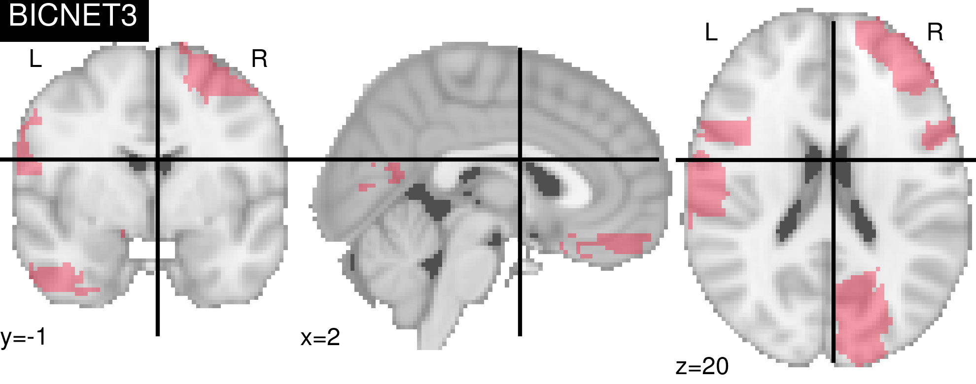
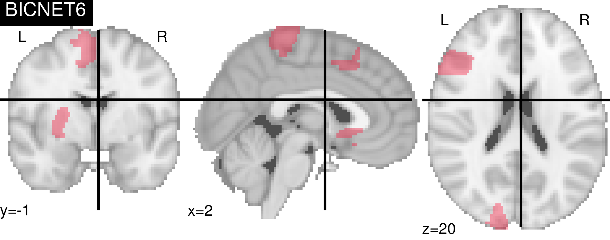
Figure 9 shows group spatial maps of ICNs 3 and 6 that are correlated to language task accuracy. The group spatial map of ICN 3 mainly consists of the language network, right frontal lobe, and occipital lobe. It indicates that though the language function is closely related to the left hemisphere, the right frontal lobe is also involved in this process and probably helps with understanding and interpretation. [34] also reports right frontal lobe activation when patients’ left hemispheres are injured. ICN 6 is mainly the language network on the left hemisphere.
These observations emphasize the fundamental role of language networks in language processing. However, language processing involves sensory input, motor output, attention, and a short-term memory system. To further understand language processing, it is necessary to analyze them in a finer functional resolution.
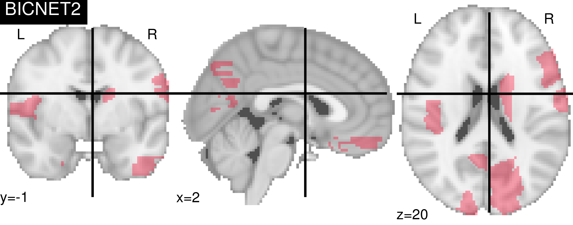
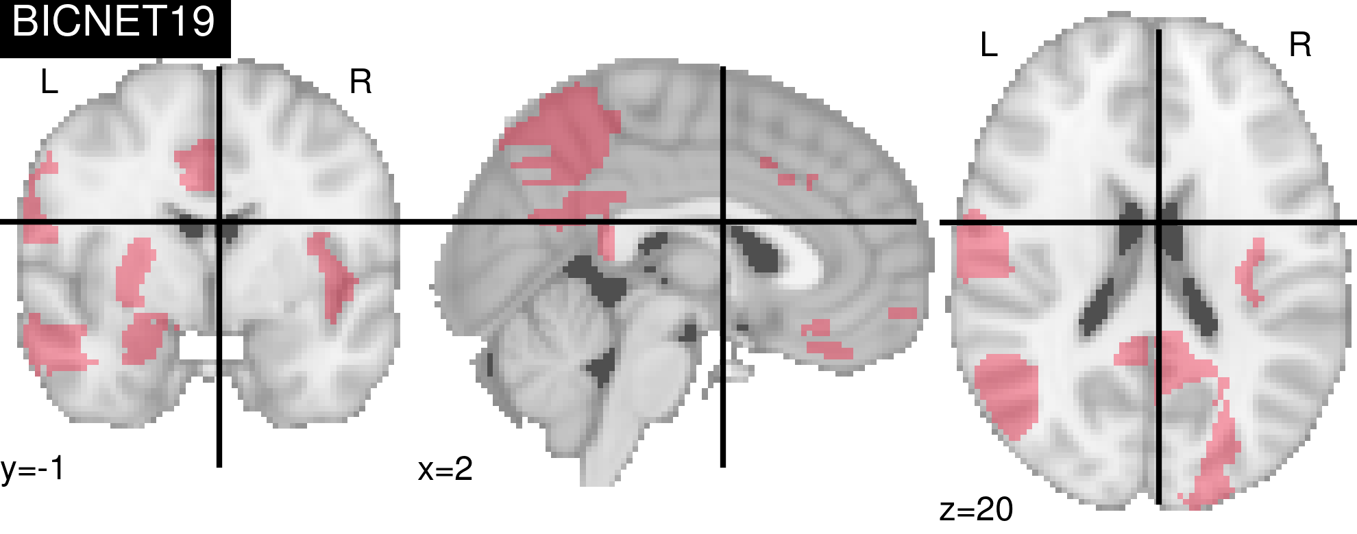
Group spatial maps of ICN 2 and 19 show interesting asymmetric patterns related to the story difficulty level. ICN 2 has main contributions from the right hemisphere. On the contrary, the group spatial map of ICN 19 focuses more on the left hemisphere, which involves the language network. It indicates that these two ICNs are related to language processing and high-level cognitive process. [35] demonstrates that vision and attention are biased toward the right hemisphere while language and internal thought are biased towards the left hemisphere. While the left brain is credited with language, the right brain helps us understand the context and tone. Also, both spatial maps involve the parietal lobe, which suggests that the parietal lobe also plays an essential role in language processing.
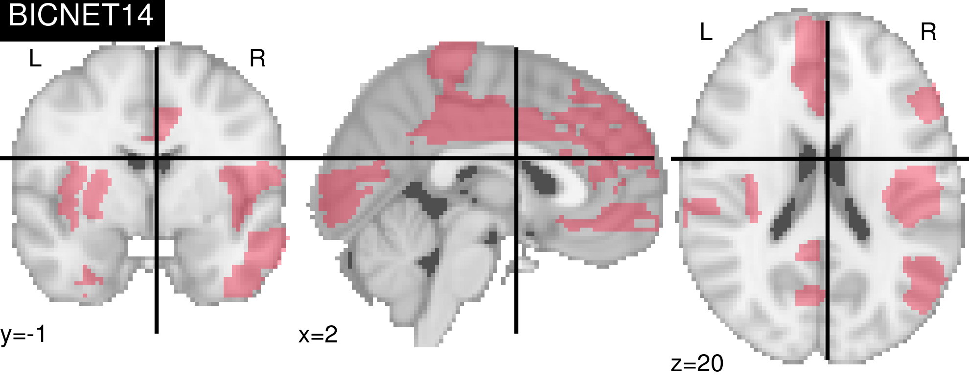
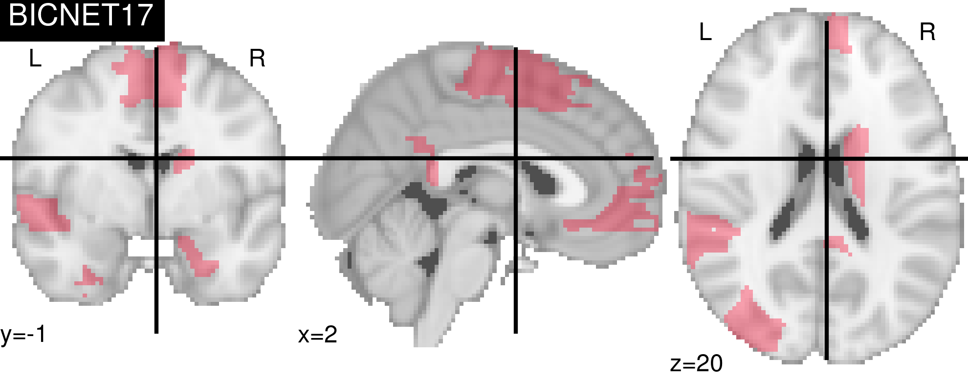
Similarly, ICNs related to math tasks’ difficulty levels are also asymmetric with group spatial map of ICN 14 focus in the right hemisphere and group spatial map of ICN 17 focus in the left hemisphere. Compared to the ICNs related to story tasks’ difficulty levels, these ICNs are mainly located in the frontal and parietal lobe.
Overall, group spatial maps related to behavioral measures tend to be asymmetric while focus on some specific regions. This phenomenon indicates the task execution requires functional integration of different regions while some specific regions still play a dominant role.
4.3.3 Comparison to group ICA spatial maps estimated by GIFT
We also estimated 20 group ICA spatial maps using the GIFT algorithm. The spatial maps estimated by GIFT are converted to the corresponding one-sample -statistics and thresholded at (, ). As shown in eq. 8, we use Jaccard similarity to measure the overlap between the spatial maps estimated by group ICA and BICNet, and thus obtain a one-to-one mapping between them.
| (8) |
where is the set of ROIs in BICNet group spatial map and is the set of ROIs in GIFT group spatial map . The average Jaccard similarity is with a standard deviation of .
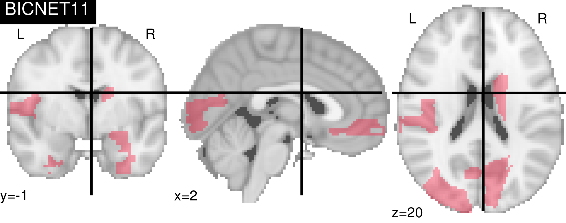


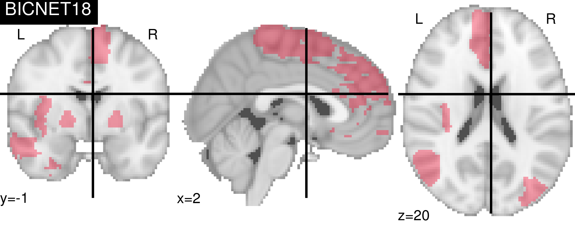

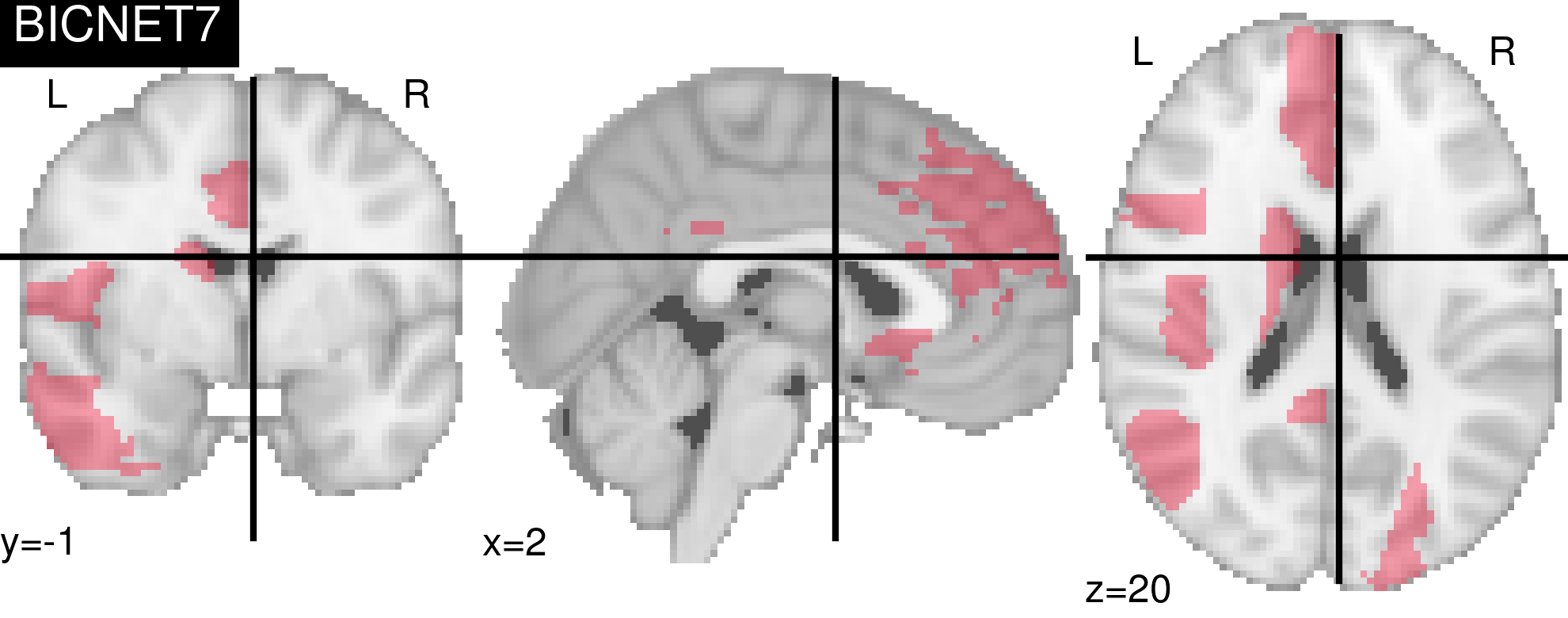

Figure 12 presents the four most similar BICNet-GIFT spatial map pairs. We notice that GIFT tends to capture symmetric parts in both hemispheres while BICNet tends to capture asymmetric integration of ROIs in two hemispheres. The asymmetry shown in this application and the statistical properties make BICNet more suitable to identify functionally meaningful ICNs.
4.3.4 Static and Dynamic Amplitudes of individual ICNs
This analysis clearly demonstrates that the BICNet model is able to detect activation states’ changes, including no activation, excitation, and inhibition, using either the static or dynamic ICN amplitudes from resting state to language task performance at the individual level.
As shown in fig. 13(a), an ICN shows of no activation, of excitation, and of inhibition across 200 subjects. The percentage of an ICN being activated across subjects is relatively low, which indicates high individual variability on ICN variation. Figure 13(b) shows that each subject has at least of ICNs remain non-activated switching from the resting state to language task execution. Figure 13(c) illustrates the inter-subject variability on ICN activation. For example, ICN 4 was activated on subject 1 and 2, inhibited on subject 3 inhibited, and had no impact on subject 4.


Figure 14 illustrates how a set of ICNs contribute to a dynamic functional brain network. Each row shows the individual difference of the same ICN under the same experimental condition. Each column shows the changes of individual ICNs contribute to a similar yet different dynamic functional connectivity. This analysis demonstrates the advantage of BICNet over group ICA methods because it provides a framework upon which we infer the ICNs with dynamic amplitudes other than just spatial maps.
In BICNet, the dynamic amplitude is measured by . In this data analysis, we label the resting period and language task period a priori by assigning the corresponding task to each time point . During the language task period, the participants were given either story or math tasks whose sequence is unknown to the BICNet a priori, as shown in fig. 15(a.

To interpret the dynamic amplitudes, we compared these to the stimulus sequence in fig. 15(a) using both time-lagged cross-correlation and change point detection. First, we calculate the time-lagged cross-correlation with lag between stimulus sequence and the dynamic amplitudes for each subject and each ICN. The time lag of maximum cross-correlation is at seconds with a standard deviation of seconds.
As shown in fig. 16, a change-point analysis was conducted using the Bayesian method in [36] where the RMSE was calculated. The Bayesian change point algorithm tends to detect more change points from the dynamic amplitudes than the real change of stimuli. The 25%, 50%, and 75% quantiles of RMSEs are 8.87 seconds, 15.58 seconds, and 30 seconds respectively, which is highly similar to the time lag estimated by the time-lagged cross-correlation above.
The results suggest a time lag for the dynamic amplitudes to adapt to the stimulus changes, and the dynamic amplitudes fluctuate more frequently than the external stimuli.


5 Conclusion
The proposed BICNet model was demonstrated to have the ability to identify individual and group-level ICN structures and quantify the task-related effect through changes in ICN amplitudes in the single-subject level. The hierarchy ICN structure is flexible enough to account for individual differences while assuming a group-level structure. The sparsity provides an interpretable ICN structure. The simulation studies demonstrate that BICNet is a potentially more informative substitute to ICA-based methods on quantifying task-related effects on a set of ICNs. In the analysis of HCP data, BICNet identified language networks across subjects and limbic networks related to emotional processing and showed high inter-subject variability. It also suggests that language task execution involves language comprehension, attention, and movement execution.
The stochastic volatility process on the ICN amplitudes assumes continuous and nonlinear brain states. Similar to ICA, BICNet can handle various types of non-Gaussianity with the stochastic volatility processes, such as sub-Gaussian and super-Gaussian distributions, and can be adapted to skewed distributions. However, BICNet does not admit multi-modal distributions because each ICN has a distinct singular functional role, which should not be mistaken for functional segregation regions of interest.
Determining the number of factors is a tricky question in latent factor modeling. Under the Bayesian framework, there are many ways to tackle the problem. One approach is to estimate the model with different ’s and then compare the samples using model selection criteria. However, this method is time- and resource-consuming and not applicable to a large-scale and complicated real-life problem. The second option is by using sparse priors that are robust against over-fitting on . For example, we can specify a large and let the sparse prior shrink the superfluous factor loadings to zero. However, this method’s robustness is yet to confirm and is also not scalable to a high-dimensional problem. The third is to adopt different MCMC sampling algorithms, such as reversible jump MCMC to explore possible . It is also a common practice in Bayesian factor analysis. [37] applied this algorithm to the Bayesian explanatory factor model and inferred the number of latent factors. More advance, we can use Bayesian nonparametric to model the unknown dimension of latent space. In terms of factor analysis, the Indian buffet process is the most commonly used [38].
The use of spike-and-slab prior gives satisfying results in terms of interpretability. However, the MCMC sampling methods tend to mix slowly due to the posterior distribution’s multi-modal nature. Also, the hidden layers in BICNet are computationally challenging. This issue can be alleviated by using approximation inference methods, including variants of variational Bayes approximations, variants of expectation propagation methods [39], and integrated nested Laplace approximations [40].
Further, in the analysis, the experimental condition is known in advance. In reality, we sometimes do not know the experimental conditions, but we are interested in inferring them. [41] proposes to use a Markov-switching model to estimate unknown stimuli sequence and apply it to the HCP language and motor tasks. However, it requires the number of experimental conditions known or estimated with model selection methods in advance. Besides, [42] proposes a Bayesian nonparametric approach for Markov-switching processes, which can also infer the number of experimental conditions. However, a Markov-switching model will add one more hidden layer to the BICNet model, making the inference more challenging. Also, Bayesian nonparametric is computationally demanding. Therefore, it is still an open question on how to infer the experimental conditions systematically and effectively.
References
- [1] S. M. Smith, P. M. T. Fox, K. L. Miller, D. C. Glahn, P. M. T. Fox, C. E. Mackay, N. Filippini, K. E. Watkins, R. Toro, A. R. Laird, C. F. Beckmann, Correspondence of the brain’s functional architecture during activation and rest, Proceedings of the National Academy of Sciences of the United States of America 106 (31) (2009) 13040–13045. doi:10.1073/pnas.0905267106.
- [2] E. M. Gordon, M. Stollstorff, C. J. Vaidya, Using spatial multiple regression to identify intrinsic connectivity networks involved in working memory performance, Human Brain Mapping 33 (7) (2012) 1536–1552. doi:10.1002/hbm.21306.
- [3] M. W. Cole, D. S. Bassett, J. D. Power, T. S. Braver, S. E. Petersen, Intrinsic and task-evoked network architectures of the human brain., Neuron 83 (1) (2014) 238–51. arXiv:NIHMS150003, doi:10.1016/j.neuron.2014.05.014.
- [4] M. Greicius, Resting-state functional connectivity in neuropsychiatric disorders, Current Opinion in Neurology 21 (4) (2008) 424–430. doi:10.1097/wco.0b013e328306f2c5.
- [5] M. D. Greicius, G. Srivastava, A. L. Reiss, V. Menon, Default-mode network activity distinguishes Alzheimer’s disease from healthy aging: Evidence from functional MRI, Proceedings of the National Academy of Sciences of the United States of America 101 (13) (2004) 4637–4642. doi:10.1073/pnas.0308627101.
- [6] S. J. Broyd, C. Demanuele, S. Debener, S. K. Helps, C. J. James, E. J. Sonuga-Barke, Default-mode brain dysfunction in mental disorders: A systematic review, Neuroscience and Biobehavioral Reviews 33 (3) (2009) 279–296. doi:10.1016/j.neubiorev.2008.09.002.
- [7] M. Goodkind, S. B. Eickhoff, D. J. Oathes, Y. Jiang, A. Chang, L. B. Jones-Hagata, B. N. Ortega, Y. V. Zaiko, E. L. Roach, M. S. Korgaonkar, S. M. Grieve, I. Galatzer-Levy, P. T. Fox, A. Etkin, Identification of a common neurobiological substrate for mental Illness, JAMA Psychiatry 72 (4) (2015) 305–315. doi:10.1001/jamapsychiatry.2014.2206.
- [8] M. D. Fox, A. Z. Snyder, J. L. Vincent, M. Corbetta, D. C. Van Essen, M. E. Raichle, The human brain is intrinsically organized into dynamic, anticorrelated functional networks, Proceedings of the National Academy of Sciences of the United States of America 102 (27) (2005) 9673–9678. doi:10.1073/pnas.0504136102.
- [9] W. W. Seeley, V. Menon, A. F. Schatzberg, J. Keller, G. H. Glover, H. Kenna, A. L. Reiss, M. D. Greicius, Dissociable intrinsic connectivity networks for salience processing and executive control, Journal of Neuroscience 27 (9) (2007) 2349–2356. doi:10.1523/JNEUROSCI.5587-06.2007.
- [10] A. Doll, B. K. Hölzel, C. C. Boucard, A. M. Wohlschläger, C. Sorg, Mindfulness is associated with intrinsic functional connectivity between default mode and salience networks, Frontiers in Human Neuroscience 9 (AUGUST) (2015) 1–11. doi:10.3389/fnhum.2015.00461.
- [11] A. R. Laird, P. M. Fox, S. B. Eickhoff, J. A. Turner, K. L. Ray, D. R. McKay, D. C. Glahn, C. F. Beckmann, S. M. Smith, P. T. Fox, Behavioral Interpretations of Intrinsic Connectivity Networks, Journal of Cognitive Neuroscience 23 (12) (2011) 4022–4037.
- [12] C. Gratton, T. O. Laumann, A. N. Nielsen, D. J. Greene, E. M. Gordon, A. W. Gilmore, S. M. Nelson, R. S. Coalson, A. Z. Snyder, B. L. Schlaggar, N. U. Dosenbach, S. E. Petersen, Functional Brain Networks Are Dominated by Stable Group and Individual Factors, Not Cognitive or Daily Variation, Neuron 98 (2) (2018) 439–452.e5. doi:10.1016/j.neuron.2018.03.035.
- [13] S. Kim, N. Shephard, S. Chib, Stochastic Volatility: Likelihood Inference and Comparison with ARCH Models, Review of Economic Studies 65 (3) (1998) 361–393. doi:10.1111/1467-937X.00050.
- [14]
G. Kastner, Sparse
Bayesian time-varying covariance estimation in many dimensions, Journal of
Econometrics 210 (1) (2019) 98–115.
doi:10.1016/j.jeconom.2018.11.007.
URL https://doi.org/10.1016/j.jeconom.2018.11.007 - [15] R. Cont, Volatility clustering in financial markets: Empirical facts and agent-based models, Long Memory in Economics (2007) 289–309.
- [16] D. A. Hsieh, Chaos and Nonlinear Dynamics: Application to Financial Markets, The Journal of Finance 46 (5) (1991) 1839–1877. doi:10.1111/j.1540-6261.1991.tb04646.x.
- [17] P. E. Vértes, R. M. Nicol, S. C. Chapman, N. W. Watkins, D. A. Robertson, E. T. Bullmore, Topological isomorphisms of human brain and financial market networks, Frontiers in Systems Neuroscience 5 (SEPTEMBER 2011) (2011) 1–12. doi:10.3389/fnsys.2011.00075.
- [18] A. Hyvärinen, E. Oja, Independent Component Analysis: Algorithms and Applications, Tech. Rep. 5 (2000).
- [19]
J. Lukemire, S. Kundu, G. Pagnoni, Y. Guo,
Bayesian
Joint Modeling of Multiple Brain Functional Networks, Journal of the
American Statistical Association (2020) 1–13arXiv:1708.02123, doi:10.1080/01621459.2020.1796357.
URL https://www.tandfonline.com/doi/full/10.1080/01621459.2020.1796357 - [20]
L. Bian, T. Cui, B. T. T. Yeo, A. Fornito, A. Razi, J. Keith,
Identification of brain states,
transitions, and communities using functional MRI (2021).
arXiv:2101.10617.
URL http://arxiv.org/abs/2101.10617 - [21]
E. I. George, R. E. McCulloch,
Variable
Selection via Gibbs Sampling, Journal of the American Statistical
Association 88 (423) (1993) 881–889.
doi:10.1080/01621459.1993.10476353.
URL http://www.tandfonline.com/doi/abs/10.1080/01621459.1993.10476353 - [22] Z. Yu, R. Prado, E. Burke, S. C. Cramer, H. Ombao, A Hierarchical Bayesian Model for Studying the Impact of Stroke on Brain Motor Function, Journal of the American Statistical Association 111 (514) (2016) 549–563. doi:10.1080/01621459.2015.1133425.Understanding.
- [23] G. Kastner, S. Frühwirth-Schnatter, H. F. Lopes, Efficient Bayesian Inference for Multivariate Factor Stochastic Volatility Models, Journal of Computational and Graphical Statistics 26 (4) (2017) 905–917. arXiv:arXiv:1602.08154v3, doi:10.1080/10618600.2017.1322091.
- [24] M. A. Lindquist, The Statistical Analysis of fMRI Data, Statistical Science 23 (4) (2008) 439–464. arXiv:0906.3662, doi:10.1214/09-STS282.
- [25]
C. Gorrostieta, H. Ombao, P. Bédard, J. N. Sanes,
Investigating
brain connectivity using mixed effects vector autoregressive models,
NeuroImage 59 (4) (2012) 3347–3355.
doi:10.1016/j.neuroimage.2011.08.115.
URL http://dx.doi.org/10.1016/j.neuroimage.2011.08.115 - [26] D. Simpson, H. Rue, A. Riebler, T. G. Martins, S. H. Sørbye, Penalising model component complexity: A principled, practical approach to constructing priors, Statistical Science 32 (1) (2017) 1–28. arXiv:1403.4630, doi:10.1214/16-STS576.
- [27] N. Klein, T. Kneib, Scale-dependent priors for variance parameters in structured additive distributional regression, Bayesian Analysis 11 (4) (2016) 1071–1106. doi:10.1214/15-BA983.
- [28] J. Hlinka, M. Paluš, M. Vejmelka, D. Mantini, M. Corbetta, Functional connectivity in resting-state fMRI: Is linear correlation sufficient?, NeuroImage 54 (3) (2011) 2218–2225. doi:10.1016/j.neuroimage.2010.08.042.
- [29] M. Welvaert, Y. Rosseel, On the definition of signal-to-noise ratio and contrast-to-noise ratio for fMRI data, PLoS ONE 8 (11) (2013). doi:10.1371/journal.pone.0077089.
- [30] G. Kastner, S. Frühwirth-Schnatter, Ancillarity-sufficiency interweaving strategy (ASIS) for boosting MCMC estimation of stochastic volatility models, Computational Statistics and Data Analysis 76 (2014) 408–423. arXiv:1706.05280, doi:10.1016/j.csda.2013.01.002.
- [31] D. C. Van Essen, K. Ugurbil, E. Auerbach, D. Barch, T. E. Behrens, R. Bucholz, A. Chang, L. Chen, M. Corbetta, S. W. Curtiss, S. Della Penna, D. Feinberg, M. F. Glasser, N. Harel, A. C. Heath, L. Larson-Prior, D. Marcus, G. Michalareas, S. Moeller, R. Oostenveld, S. E. Petersen, F. Prior, B. L. Schlaggar, S. M. Smith, A. Z. Snyder, J. Xu, E. Yacoub, The Human Connectome Project: A data acquisition perspective, NeuroImage 62 (4) (2012) 2222–2231. doi:10.1016/j.neuroimage.2012.02.018.
- [32] M. Glasser, The Human Connectome Project: Progress and Prospects, Cerebrum: the Dana Forum on Brain Science 2016 (September) (2016) 1–16.
- [33]
M. F. Glasser, S. N. Sotiropoulos, J. A. Wilson, T. S. Coalson, B. Fischl,
J. L. Andersson, J. Xu, S. Jbabdi, M. Webster, J. R. Polimeni, D. C. Van
Essen, M. Jenkinson,
The minimal
preprocessing pipelines for the Human Connectome Project, NeuroImage 80
(2013) 105–124.
doi:10.1016/j.neuroimage.2013.04.127.
URL http://dx.doi.org/10.1016/j.neuroimage.2013.04.127 - [34]
N. L. Voets, J. E. Adcock, D. E. Flitney, T. E. J. Behrens, Y. Hart, R. Stacey,
K. Carpenter, P. M. Matthews,
Distinct
right frontal lobe activation in language processing following left
hemisphere injury, Brain 129 (3) (2006) 754–766.
doi:10.1093/brain/awh679.
URL http://academic.oup.com/brain/article/129/3/754/390767/Distinct-right-frontal-lobe-activation-in-language - [35]
M. C. Corballis, Left
Brain, Right Brain: Facts and Fantasies, PLoS Biology 12 (1) (2014)
e1001767.
doi:10.1371/journal.pbio.1001767.
URL https://dx.plos.org/10.1371/journal.pbio.1001767 - [36] C. Erdman, J. W. Emerson, bcp: An R package for performing a bayesian analysis of change point problems, Journal of Statistical Software 23 (3) (2007) 1–13. doi:10.18637/jss.v023.i03.
- [37]
G. Conti, S. Frühwirth-Schnatter, J. J. Heckman, R. Piatek,
Bayesian exploratory
factor analysis, Journal of Econometrics 183 (1) (2014) 31–57.
doi:10.1016/j.jeconom.2014.06.008.
URL http://dx.doi.org/10.1016/j.jeconom.2014.06.008 - [38] D. Knowles, Z. Ghahramani, Nonparametric Bayesian sparse factor models with application to gene expression modeling, Annals of Applied Statistics 5 (2 B) (2011) 1534–1552. doi:10.1214/10-AOAS435.
- [39] O. Stegle, K. Sharp, J. Winn, A Comparison of Inference in Sparse Factor Analysis, Journal of Machine Learning Research 1 (2000) 1–48.
- [40]
H. Rue, S. Martino, N. Chopin,
Approximate
Bayesian inference for latent Gaussian models by using integrated nested
Laplace approximations, Journal of the Royal Statistical Society. Series B:
Statistical Methodology 71 (2) (2009) 319–392.
doi:10.1111/j.1467-9868.2008.00700.x.
URL https://rss.onlinelibrary.wiley.com/doi/full/10.1111/j.1467-9868.2008.00700.xhttps://rss.onlinelibrary.wiley.com/doi/abs/10.1111/j.1467-9868.2008.00700.xhttps://rss.onlinelibrary.wiley.com/doi/10.1111/j.1467-9868.2008.00700.x - [41]
C.-M. Ting, S. B. Samdin, M. Tang, H. Ombao,
Detecting Dynamic Community
Structure in Functional Brain Networks Across Individuals: A Multilayer
Approach, IEEE Transactions on Medical Imaging (2020) 1–1arXiv:2004.04362, doi:10.1109/TMI.2020.3030047.
URL http://arxiv.org/abs/2004.04362https://ieeexplore.ieee.org/document/9220100/ - [42] E. Fox, E. Sudderth, M. Jordan, A. Willsky, Bayesian nonparametric methods for learning markov switching processes, IEEE Signal Processing Magazine 27 (6) (2010) 43–54. doi:10.1109/MSP.2010.937999.