跳到论文正文
W Papers独立论文阅读器 arXiv:2107.09054 论文正文 计算阅读时间 · 0%
引用这篇论文根据当前论文元数据生成,正式投稿前建议核对。


License: CC BY-NC-ND 4.0
arXiv:2107.09054v1 [math-ph] 18 Jul 2021

Obtaining the long-term behavior of Master equations with finite state space from the structure of the associated state transition network

Bernd Fernengel Affiliation: Institut für Festkörperphysik Affiliation: Technische Universität Darmstadt Affiliation: Hochschulst. 6, 64289 Darmstadt, Germany Email: bernd@pkm.tu-darmstadt.de    Barbara Drossel Affiliation: Institut für Festkörperphysik Affiliation: Technische Universität Darmstadt Affiliation: Hochschulst. 6, 64289 Darmstadt, Germany Email: drossel@pkm.tu-darmstadt.de
Abstract

The Master equation describes the time evolution of the probabilities of a system with a discrete state space. This time evolution approaches for long times a stationary state that will in general depend on the initial probability distribution. Conditions under which the stationary state is unique are usually given as remarks appended to more comprehensive theories in the mathematical literature. We provide a direct and complete derivation of a necessary and sufficient criterion for when this steady state is unique. We translate this problem into the language of graph theory and show that there is a one-to-one correspondence between minimal absorbing sets within the state-transition network and linearly independent stationary states of the Master equation.

Keywords Master equation ⋅\cdot relaxing ⋅\cdot steady states ⋅\cdot connectivity ⋅\cdot absorbing subnetworks

1 Introduction

Master equations appear in many different context in chemistry, biology and physics. Examples are biochemical reaction networks, stochastic population dynamics based on deaths and births, and various statistical physics problems.

Master equations describe the time evolution of the probabilities of the different states of a system, with the dynamics being due to transitions between these states [1, 2]. The most common form is an initial value problem of a linear differential equation. The picture behind a Master equation is that of probabilities flowing between states like a fluid, where their total amount is being conserved. The probability flow along a directed link depends linearly on the strength of the link and the amount of probability at the source. Of particular interest is the long-time behaviour of the solution, as this determines the states where a system will eventually be, together with their probabilities. Unlike discrete-time Markov chains, which can lead to long-term oscillations of the probabilities, the solution of the Master equation for a finite state space will always converge to a stationary solution where the probability distribution does not change any more. In general, this steady state will depend on the initial distribution of the probabilities, i.e., on the initial condition of the corresponding differential equation.

In this paper we focus on the question under which conditions a finite-size Master equation has a unique steady state, in which case the Master equation is called relaxing [3].

The mathematical literature contains necessary and sufficient conditions for the stationary state to be unique, but these are only hinted at or given as a remark appended to theorems within major treatises on topics such as Master equations, Markov chains or directed graphs [4, 5, 6]. What these all lack is a clear statement and proof that is based on first principles.

In the physical literature, usually more special situations are discussed. For instance, the Master equation for the microcanonical ensemble of statistical physics can be shown to be relaxing because the transition rates between pairs of states are symmetric. Therefore, the steady state is the uniform distribution [1, 2].

The often-cited review by Schnakenberg on the network theory of Master equation systems [7] discusses models where to each transition there exists also the reverse transition. In this specific case, the stationary solution is always unique. A more mathematical paper by Jamilowski and Staszewski [8] gives a general criterion for the Master equation to be relaxing, however, this criterion is a nonintuitive mathematical expression based on the principal minors of the matrix that contains the transition rates.

Our goal in this paper is to provide a direct proof that is accessible for physicists without delving deep into the mathematical literature. This proof proceeds by translating the initial value problem into the language of graph theory. By considering the network of the states of the system and the transitions between them, an intuitive understanding of the meaning of the steps of the proof can be achieved. An important notion is that of minimal absorbing sets, which are subsets of states from where the probability cannot escape. We show that the number of linearly independent steady states of the Master equation equals the number of minimal absorbing sets in the corresponding transition network. In particular, the steady state of the Master equation is unique if and only if there is exactly one minimal absorbing set. While this statement seems intuitively clear, the complete proof is non-trivial, even though it uses only undergraduate mathematics.

2 The Master equation and the time evolution operator

We consider a system of N∈ℕN\in\mathbb{N} states and the transitions between them. If there is no transition from state ii to state jj, the associated transition rate γi→j\gamma_{i\to j} vanishes. The states and the nonzero transition rates form together a network 𝒮=(Ω,ℰ)\mathcal{S}=(\Omega,\mathcal{E}), with the states Ω={1,…,N}\Omega=\{1,\dotsc,N\} being the nodes and the transitions being the directed links ℰ⊆Ω×Ω\mathcal{E}\subseteq\Omega\times\Omega of the network. The transition rates indicate the weights of these links. For all subsets of states B⊆ΩB\subseteq\Omega there is a corresponding subnetwork (B,ℰB)(B,\mathcal{E}_{B}), where ℰB:={(i,j)∈ℰ:i,j∈B}\mathcal{E}_{B}:=\{(i,j)\in\mathcal{E}\,:\,i,j\in B\} consists of all links in the subset B⊆ΩB\subseteq\Omega.

Since transitions occur only between different states, the network has no self-loops, that is γi→i=0\gamma_{i\to i}=0 for all i∈Ωi\in\Omega.

We denote with pi​(t)p_{i}(t) the probability of the system to be in state ii at time t. These probabilities are nonnegative and normalized, 𝐩∈[0,1]N​ with ​‖𝐩‖1=1\mathbf{p}\in[0,1]^{N}\,\text{ with }\|\mathbf{p}\|_{1}=1.

The Master equation that describes the change in time of these probabilities is the following initial value problem

∂tpi​(t)\displaystyle\partial_{t}p_{i}(t) =∑j=1j≠iN(pj​(t)​γj→i−pi​(t)​γi→j)\displaystyle={\sum}\limits_{j=1\atop j\neq i}^{N}\;\big(\,p_{j}(t)\,\gamma_{j\to i}-p_{i}(t)\,\gamma_{i\to j}\,\big) (1)
pi​(t=0)\displaystyle p_{i}(t=0) =p0(i),\displaystyle=p^{(i)}_{0},

or, in matrix-vector notation,

𝐩˙\displaystyle\dot{\mathbf{p}} =Γ​𝐩\displaystyle=\,\Gamma\,\mathbf{p} (2)
𝐩⁡(t=0)\displaystyle\mathbf{p}(t=0) =𝐩0, with ​Γi​j={γj→i,i≠j−∑k=1Nγj→k,i=j.\displaystyle=\mathbf{p}_{0},\text{ with }\Gamma_{ij}=\,\begin{cases}\gamma_{j\to i}&,i\neq j\\ -{\sum}\limits_{k=1}^{N}\gamma_{j\to k}&,i=j\,.\end{cases}

The solution is given by 𝐩t:=eΓ​t​𝐩0\mathbf{p}_{t}:=\text{e}^{\Gamma\,t}\,\mathbf{p}_{0}, with the initial state 𝐩⁡(t=0)=𝐩0\mathbf{p}(t=0)=\mathbf{p}_{0} and the solution operator

eΓ​t:=∑k∈ℕ0Γk​tkk!=limn→∞(ℐ+Γ​tn)n.\displaystyle\text{e}^{\Gamma\,t}:={\sum}\limits_{k\in\mathbb{N}_{0}}\frac{\Gamma^{k}\,t^{k}}{k!}=\lim\limits_{n\to\infty}\left(\mathcal{I}+\frac{\Gamma\,t}{n}\right)^{n}. (3)

The matrix Γ\Gamma is called the generator of the network Ω\Omega [4].

In the following, we relate properties of the solution 𝐩t:=eΓ​t​𝐩0\mathbf{p}_{t}:=\text{e}^{\Gamma\,t}\,\mathbf{p}_{0} to the properties of the network Ω\Omega.

Since the column sum of Γ\Gamma is zero (∑i=1NΓi​j=0)\left(\sum\limits_{i=1}^{N}\Gamma_{ij}=0\right), the matrix Γ\Gamma has at least one eigenvalue 0. The eigenvectors to this eigenvalue are stationary states that satisfy 𝐩˙=0\dot{\mathbf{p}}=0. From Gershgorin’s circle theorem [9] follows that all non-zero eigenvalues of Γ\Gamma have a (strictly) negative real part.

The column sum of any matrix power of Γ\Gamma is also zero, ∑i=1N(Γk)i​j=0\sum\limits_{i=1}^{N}\left(\Gamma^{k}\right)_{ij}=0 for all k∈ℕk\in\mathbb{N}, as can be shown by induction. Further, a power series expansion yields that the column sums of its matrix exponential eΓ​t\text{e}^{\Gamma\,t} equals one,

∑i=1N(eΓ​t)i​j=1.\sum\limits_{i=1}^{N}\left(\text{e}^{\Gamma\,t}\right)_{ij}=1. (4)

Every initial state can be written as a linear combination of generalized eigenvectors of Γ\Gamma. In the limit t→∞t\to\infty, only the eigenvectors of the eigenvalue λ=0\lambda=0 ( the ones lying in the kernel of Γ\Gamma) remain, while the contributions of the other eigenvectors decay exponentially.

To see this, let 𝐯λ,m\mathbf{v}_{\lambda,m} be a generalized eigenvector of rank m∈ℕm\in\mathbb{N} to the eigenvalue λ\lambda. The action of the time evolution operator eΓ​t\text{e}^{\Gamma\,t} on this vector is

eΓ​t​𝐯λ,m=eλ​t​∑k=0m−1tkk!​𝐯λ,m−k.\displaystyle\text{e}^{\Gamma\,t}\,\mathbf{v}_{\lambda,m}=\text{e}^{\lambda\,t}\,\sum\limits_{k=0}^{m-1}\frac{t^{k}}{k!}\,\mathbf{v}_{\lambda,m-k}\,. (5)

For non-zero eigenvalues λ≠0\lambda\neq 0, this tends to zero since Re​[λ]< 0\text{Re}[\lambda]\,<\,0. For λ=0\lambda=0, we must have m=1m=1 since the solution of the master equation (2) is bounded. This means that all generalized eigenvectors to the eigenvalue λ=0\lambda=0 lie in the kernel of Γ\Gamma.

This results in

eΓ​t​𝐯λ=0=𝐯λ=0.\displaystyle\text{e}^{\Gamma\,t}\,\mathbf{v}_{\lambda=0}=\mathbf{v}_{\lambda=0}\,. (6)

3 Definitions and preparatory considerations

Before we can state and prove the main theorem, we need a few more definitions and theorems.

3.1 Paths

If state bb can be reached from state aa via a series of transitions, there is a path from aa to bb, which we indicate by a↝ba\rightsquigarrow b, and we say that state bb is reachable from state aa. We denote with

  • •

    ℛ(→a):={b∈Ω|b↝a}\mathcal{R}(^{\rightarrow}a):=\{b\in\Omega\,|\,b\rightsquigarrow a\} the set of states from where a path to aa exists and with

  • •

    ℛ⁡(a→):={b∈Ω|a↝b}\mathcal{R}(a^{\rightarrow}):=\{b\in\Omega\,|\,a\rightsquigarrow b\} the set of states to which a path from aa exists.

3.2 Weak, unilateral, and strong connectedness

We call Ω\Omega

  • i)

    weakly connected if the corresponding undirected graph of Ω\Omega is connected;

  • ii)

    unilaterally connected if for all a,b∈Ωa,\,b\in\Omega, bb is reachable from aa OR aa is reachable from bb;

  • iii)

    strongly connected if for all a,b∈Ωa,\,b\in\Omega, bb is reachable from aa and aa is reachable from bb,
    a↝b​ AND ​b↝aa\rightsquigarrow b\text{ {AND} }b\rightsquigarrow a.

Figure 1 illustrates the difference.

(a) weakly, but not unilaterally connected
Refer to caption
(b) unilaterally, but not strongly connected
Refer to caption
Figure 1: The differences between weak, unilateral and strong connectivity.

3.3 Relaxing networks

We call Ω\Omega relaxing if there exists a unique stationary state 𝐩∞\mathbf{p}_{\infty} such that for all initial conditions 𝐩0\mathbf{p}_{0} the dynamics of the Master equation converges to this stationary state, that is limt→∞𝐩t=𝐩∞\lim\limits_{t\to\infty}\mathbf{p}_{t}=\mathbf{p}_{\infty}. This means that the eigenspace of Γ\Gamma corresponding to the eigenvalue 00 is one-dimensional, dim​( kern ​(Γ))=1\text{dim}\left(\text{\,kern }(\Gamma)\right)=1.

3.4 Absorbing subsets

We write 𝐩∈B\mathbf{p}\in B if all mass of the probability distribution is restricted to a subset B∈ΩB\in\Omega, that is ∑i∈Bpi=1{\sum}\limits_{i\in B}p_{i}=1. We call a subset B⊆ΩB\subseteq\Omega absorbing if there are no edges pointing out of BB, that is if γi→j=0\gamma_{i\to j}=0 for all i∈Bi\in B and j∈BCj\in B^{C}. This means that probability cannot flow out of BB, so when the mass of the probability distribution of the initial state is in BB (𝐩0∈B\mathbf{p}_{0}\in B), then it will stay in BB for all times: 𝐩t∈B\mathbf{p}_{t}\in B for all t≥0t\geq 0.

Later, we will use the fact that ℛ(→a)C\mathcal{R}(^{\rightarrow}a)^{C} and ℛ⁡(a→)\mathcal{R}(a^{\rightarrow}) are absorbing subsets. The two statements are shown as follows:

  • •

    If ℛ(→a)C\mathcal{R}(^{\rightarrow}a)^{C} were not absorbing, there would be a state c∈ℛ(→a)Cc\in\mathcal{R}(^{\rightarrow}a)^{C} and a b∈ℛ(→a)b\in\mathcal{R}(^{\rightarrow}a) such that c↝bc\rightsquigarrow b. However, this would imply c↝b↝ac\rightsquigarrow b\rightsquigarrow a, which is a contradiction.

  • •

    If ℛ⁡(a→)\mathcal{R}(a^{\rightarrow}) were not absorbing, there would be a state b∈ℛ⁡(a→)b\in\mathcal{R}(a^{\rightarrow}) and a state c∈ℛ​(a→)Cc\in\mathcal{R}(a^{\rightarrow})^{C} such that b↝cb\rightsquigarrow c. However, this would imply a↝b↝ca\rightsquigarrow b\rightsquigarrow c, which is a contradiction.

3.5 Minimal absorbing subsets

An absorbing subset B⊆ΩB\subseteq\Omega is called minimal if for all absorbing subsets C⊆ΩC\subseteq\Omega with C⊆BC\subseteq B, we have B=C.B=C. In particular, there can be more than one minimal absorbing subset.

Every minimal absorbing subset BB is strongly connected. To see this, assume that there are two states i,j∈Bi,\,j\in B with i​\nrightsquigarrow​ji\nrightsquigarrow j. Then i∈(ℛ(→j)C∩B)i\in\left(\mathcal{R}(^{\rightarrow}j)^{C}\cap\,B\right) and j∉(ℛ(→j)C∩B)j\notin\left(\mathcal{R}(^{\rightarrow}j)^{C}\cap\,B\right). This implies that (ℛ(→j)C∩B)\left(\mathcal{R}(^{\rightarrow}j)^{C}\cap\,B\right) is a non-empty intersection of two minimal absorbing sets which is strictly less than BB, in contradiction with the premise that BB is minimal.

Every state ω∈Ω\omega\in\Omega leads to a (not necessarily unique) minimal absorbing subnetwork BωB_{\omega}, that is there exists a path ω→b\omega\to b to some element b∈Bωb\in B_{\omega} of some minimal absorbing subset BωB_{\omega}. This follows from the result in the previous subsection that the set ℛ⁡(ω→)\mathcal{R}(\omega^{\rightarrow}) is absorbing. This set must contain a minimal absorbing set Bω⊆ℛ⁡(ω→)B_{\omega}\subseteq\mathcal{R}(\omega^{\rightarrow}), and (since minimal absorbing subnetworks are strongly connected) every state of BωB_{\omega} is reachable from ω\omega, that is ω↝b\omega\rightsquigarrow b for all states b∈Bω⊆ℛ⁡(ω→)b\in B_{\omega}\subseteq\mathcal{R}(\omega^{\rightarrow}).

3.6 Diagonal dominance

Let B∈ℂN×NB\in\mathbb{C}^{N\times N} be a complex matrix.

  • •

    For i∈{1,…,N}i\in\{1,\dots,N\}, we call the ii-th row of BB strictly diagonal dominant (SDD) if |Bi​i|>∑j=1,j≠iN|Bi​j||B_{ii}|>\sum\limits_{j=1,\atop j\neq i}^{N}|B_{ij}|.

  • •

    We call the matrix BB strictly diagonal dominant (SDD) if every row of BB is SDD. Due to the Gershgorin circle theorem [9], a SDD matrix is non-singular.

  • •

    The definition of a weakly diagonal dominant (WDD) matrix is the same as the previous one, but with a "≥\geq" sign instead of a ">" sign.

  • •

    We call BB weakly chained diagonal dominant (WCDD) if BB is WDD and for all rows i∈{1,…,N}i\in\{1,\dots,N\} that are not (SSD), there exists a k∈{1,…,N}k\in\{1,\dots,N\} and a path i=i0→…→ik=ji=i_{0}\to\dots\to i_{k}=j in the directed graph associated to BB to a (SSD) row j∈{1,…,N}j\in\{1,\dots,N\} of BB.

It can be shown that WCDD matrices are non-singular ( see section (A.1) in the Appendix for a proof).

3.7 Structure of the matrix Γ\Gamma

Below, we will use the matrix Γ\Gamma in a specific form that can be obtained by re-numbering the states.

Let ℬ={B1,…,Bn},n≤N\mathcal{B}=\{B_{1},\dots,B_{n}\},\,n\leq N be the set of minimal absorbing subsets and define M:=N−∑i=1n|Bi|M:=N-\sum\limits_{i=1}^{n}|B_{i}|. We number the states as follows: The first MM states are those not contained in minimal absorbing networks. Then we count the states which lie in minimal absorbing networks block-wise, that is

B0\displaystyle{B_{0}} :=Ω\⋃i=1nBi={1,…,M}\displaystyle:=\Omega\backslash\bigcup\limits_{i=1}^{n}B_{i}=\,\{1,\dots,M\} (7)
Bi\displaystyle B_{i} ={M+∑j=1i−1|Bj|+1,…,M+∑j=1i|Bj|}, for i∈{1,…,n}.\displaystyle=\{M+{\sum}\limits_{j=1}^{i-1}|B_{j}|+1,\dots,M+{\sum}\limits_{j=1}^{i}|B_{j}|\,\},{\text{ for }i\in\{1,\dotsc,n\}}.

After this re-numbering of the states, we can write Γ\Gamma in the following form

Γ\displaystyle\Gamma =(ΓB0𝟎M×|B1|…𝟎M×|Bn|ΓB0→B1ΓB1𝟎|B1|×|B1|⋱ΓB0→Bn𝟎|Bn|×|B1|ΓBn)​ with the matrices\displaystyle=\begin{pmatrix}\Gamma_{B_{0}}&\mathbf{0}^{M\times|B_{1}|}&\dots&\mathbf{0}^{M\times|B_{n}|}\\ \Gamma_{B_{0}\to B_{1}}&\Gamma_{B_{1}}&&\mathbf{0}^{|B_{1}|\times|B_{1}|}\\ \vdots&&\ddots&\\ \Gamma_{B_{0}\to B_{n}}&\mathbf{0}^{|B_{n}|\times|B_{1}|}&&\Gamma_{B_{n}}\end{pmatrix}\text{ with the matrices } (8)
ΓB0∈ℝM×M,ΓBi\displaystyle\Gamma_{B_{0}}\in\mathbb{R}^{M\times M},\,\Gamma_{B_{i}} ∈ℝ|Bi|×|Bi|​ and ​ΓB0→Bi∈ℝ(N−M)×M, for ​i∈{1,…,n}\displaystyle\in\mathbb{R}^{|B_{i}|\times|B_{i}|}\text{ and }\Gamma_{B_{0}\to B_{i}}\in\mathbb{R}^{(N-M)\times M},\text{ for }i\in\{1,\dotsc,n\}

If there is no matrix ΓB0\Gamma_{B_{0}} (M=0)(M=0) and there is only one minimal absorbing set (n=1)(n=1), then Γ\Gamma is called irreducible [9, 10], otherwise it is called reducible.

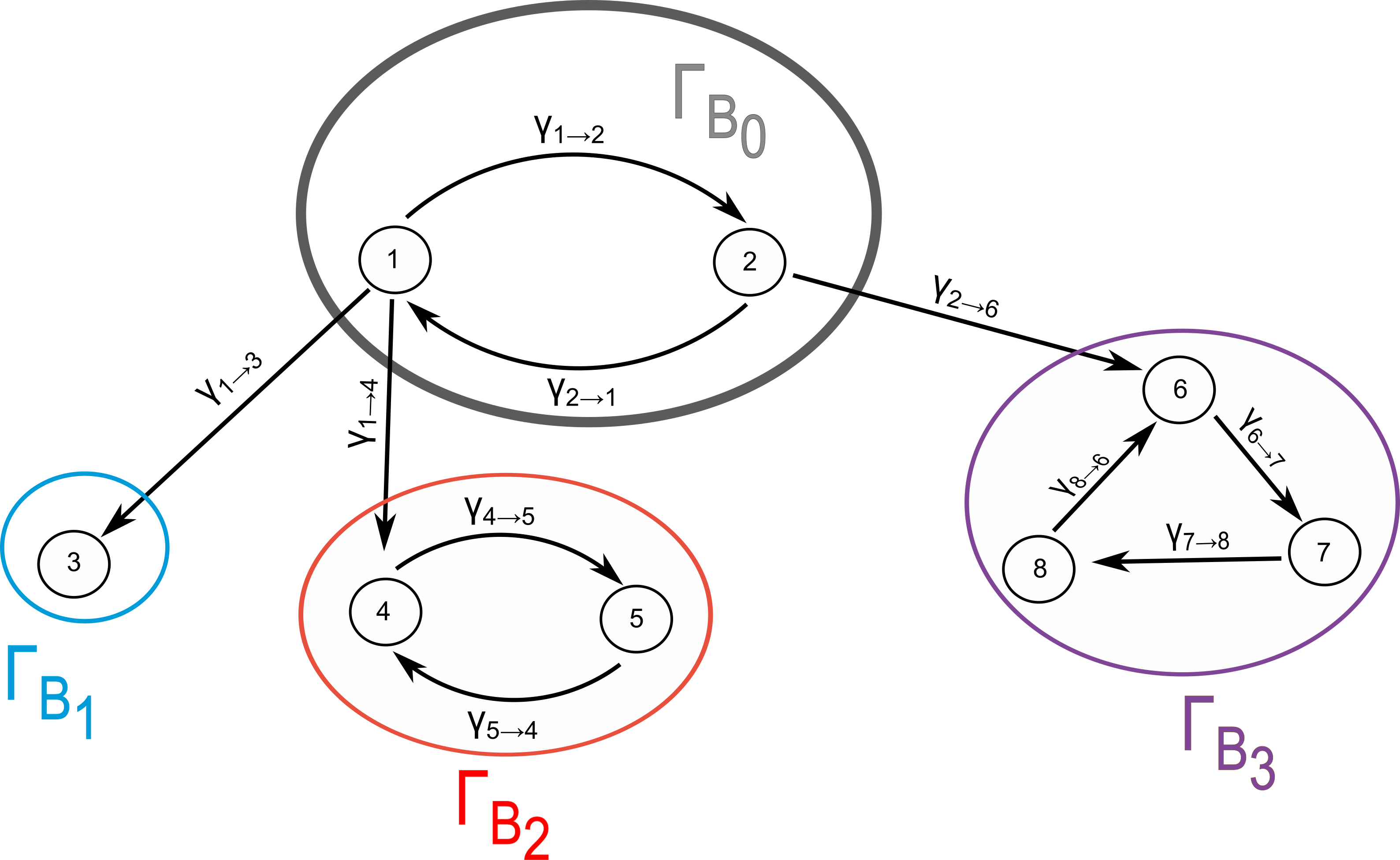
Figure 2 gives an illustrating example.
Refer to caption
Figure 2: Example of a network / directed graph with the minimal absorbing sets being B1={3}B_{1}=\{3\}, B2={4, 5}B_{2}=\{4,\,5\} and B3={6, 7, 8}B_{3}=\{6,\,7,\,8\}.

The matrices of the absorbing subnetworks and the full matrix Γ\Gamma for this example are

ΓB1=0,ΓB2=(−γ4→5γ5→4γ4→5−γ5→4),ΓB3=(−γ6→70γ8→6γ6→7−γ7→800γ7→8−γ8→6)\displaystyle{\color[rgb]{0,0.5156,0.8008}\Gamma_{B_{1}}=0},\;{\color[rgb]{0.9023,0,0.1016}\Gamma_{B_{2}}=\begin{pmatrix}-\gamma_{4\to 5}&\hskip 8.53581pt\gamma_{5\to 4}\\ \hskip 8.53581pt\gamma_{4\to 5}&-\gamma_{5\to 4}\end{pmatrix}},\;{\color[rgb]{0.5,0.2695,0.5938}\Gamma_{B_{3}}=\begin{pmatrix}-\gamma_{6\to 7}&\hskip 5.69054pt0&\hskip 8.53581pt\gamma_{8\to 6}\\ \hskip 8.53581pt\gamma_{6\to 7}&-\gamma_{7\to 8}&\hskip 5.69054pt0\\ \hskip 5.69054pt0&\hskip 8.53581pt\gamma_{7\to 8}&-\gamma_{8\to 6}\end{pmatrix}}

and

Γ=(ΓB0000ΓB0→B1ΓB100ΓB0→B20ΓB20ΓB0→B300ΓB3)=(−γ1→2−γ1→3−γ1→4γ2→1000000γ1→2−γ2→1−γ2→6000000γ1→30000000γ1→400−γ5→4γ4→5000000γ5→4−γ4→50000γ2→6000−γ6→70γ8→600000γ6→7−γ7→80000000γ7→8−γ8→6)\displaystyle\Gamma=\begin{pmatrix}\Gamma_{B_{0}}&0&0&0\\ \Gamma_{B_{0}\to B_{1}}&{\color[rgb]{0,0.5156,0.8008}\Gamma_{B_{1}}}&0&0\\ \Gamma_{B_{0}\to B_{2}}&0&{\color[rgb]{0.9023,0,0.1016}\Gamma_{B_{2}}}&0\\ \Gamma_{B_{0}\to B_{3}}&0&0&{\color[rgb]{0.5,0.2695,0.5938}\Gamma_{B_{3}}}\end{pmatrix}=\begin{pmatrix}-\gamma_{1\to 2}-\gamma_{1\to 3}-\gamma_{1\to 4}&\gamma_{2\to 1}&0&0&0&0&0&0\\ \gamma_{1\to 2}&-\gamma_{2\to 1}-\gamma_{2\to 6}&0&0&0&0&0&0\\ \gamma_{1\to 3}&0&{\color[rgb]{0,0.5156,0.8008}0}&0&0&0&0&0\\ \gamma_{1\to 4}&0&0&{\color[rgb]{0.9023,0,0.1016}-\gamma_{5\to 4}}&{\color[rgb]{0.9023,0,0.1016}\gamma_{4\to 5}}&0&0&0\\ 0&0&0&{\color[rgb]{0.9023,0,0.1016}\gamma_{5\to 4}}&{\color[rgb]{0.9023,0,0.1016}-\gamma_{4\to 5}}&0&0&0\\ 0&\gamma_{2\to 6}&0&0&0&{\color[rgb]{0.5,0.2695,0.5938}-\gamma_{6\to 7}}&{\color[rgb]{0.5,0.2695,0.5938}0}&{\color[rgb]{0.5,0.2695,0.5938}\gamma_{8\to 6}}\\ 0&0&0&0&0&{\color[rgb]{0.5,0.2695,0.5938}\gamma_{6\to 7}}&{\color[rgb]{0.5,0.2695,0.5938}-\gamma_{7\to 8}}&{\color[rgb]{0.5,0.2695,0.5938}0}\\ 0&0&0&0&0&{\color[rgb]{0.5,0.2695,0.5938}0}&{\color[rgb]{0.5,0.2695,0.5938}\gamma_{7\to 8}}&{\color[rgb]{0.5,0.2695,0.5938}-\gamma_{8\to 6}}\\ \end{pmatrix}

3.8 If the matrix ΓB0\Gamma_{B_{0}} exists, it is invertible

In order to show that the matrix ΓB0\Gamma_{B_{0}} is invertible, it suffices to show that ΓB0\Gamma_{B_{0}} is WCDD (see section (A.1) in the Appendix). We assume that Γ\Gamma is of the form (8) and ℬ={B1,…,Bn}\mathcal{B}=\{B_{1},\dotsc,B_{n}\} is the set of minimal absorbing subsets.

  • 1)

    ΓB0\Gamma_{B_{0}} is WDD, since

    ∑i=1,i≠jM|(ΓB0)i​j|⏟|Γi​j|≤∑i=1,i≠jN|Γi​j|=|Γj​j|=|(ΓB0)j​j|.\sum\limits_{i=1,\atop i\neq j}^{M}\underbrace{|\left(\Gamma_{B_{0}}\right)_{ij}|}_{|\Gamma_{ij}|}\leq\sum\limits_{i=1,\atop i\neq j}^{N}|\,\Gamma_{ij}\,|=|\,\Gamma_{jj}\,|=|\,\left(\Gamma_{B_{0}}\right)_{jj}\,|.
  • 2)

    Let x∈B0x\in B_{0} be an arbitrary state in B0B_{0}. Then there are two cases:

    • i)

      If γx→b>0\gamma_{x\to b}>0 for some b∈Bib\in B_{i}, then the xx-th row is SDD, since

      ∑i=1,i≠xM|(ΓB0)i,x|⏟|Γi,x|<∑i=1,i≠xM|Γi,x|+|Γb,x|⏟γx→b≤∑i=1,i≠xN|Γi,x|=|Γx,x|=|(ΓB0)x,x|.\sum\limits_{i=1,\atop i\neq x}^{M}\underbrace{|\left(\Gamma_{B_{0}}\right)_{i,\,x}|}_{|\Gamma_{i,\,x}|}<\sum\limits_{i=1,\atop i\neq x}^{M}|\Gamma_{i,\,x}|+\underbrace{|\Gamma_{b,\,x}|}_{\gamma_{x\to b}}\leq\sum\limits_{i=1,\atop i\neq x}^{N}|\Gamma_{i,\,x}|=|\Gamma_{x,\,x}|=|\left(\Gamma_{B_{0}}\right)_{x,\,x}|.
    • ii)

      If the xx-th column is not SSD (γx→b=0CLOSE(\gamma_{x\to b}=0 for all b∈Ω\B0b\in\Omega\backslash B_{0}, we know from section (3.5) that there exists a path from the state xx to a minimal absorbing set BiB_{i}, that is x→…→x′→bx\to\dotsc\to x^{\prime}\to b for some i∈{1,…,n}i\in\{1,\dotsc,n\} and some state b∈Bib\in B_{i} and x′∈B0x^{\prime}\in B_{0}. But this again means that if the xx-column is not SDD, there is a path from xx to the SDD column x′x^{\prime} (where γx′→b>0\gamma_{x^{\prime}\to b}>0, for some b∈Bib\in B_{i}).

    Hence, we conclude that ΓB0\Gamma_{B_{0}} is WCDD and therefore invertible.

4 A simplified version of the main theorem

Before stating the general condition for a network Ω\Omega to be relaxing, we first consider the important special case that Ω\Omega is strongly connected. Our goal in this section is to prove that a strongly connected network is relaxing (which is a corollary of the theorem of Perron-Frobenius [9]). We proceed in three steps.

4.1 A directed graph Ω\Omega is strongly connected if and only if its adjacency matrix AA is irreducible

Here, we use a different but equivalent characterization of irreducibility than above: A matrix A∈ℝN×NA\in\mathbb{R}^{N\times N} with non-negative entries (Ai​j≥ 0​ for all ​i,j)(A_{ij}\geq\,0\text{ for all }i,j) is irreducible if and only if for all i,j∈{1,…,N}i,j\in\{1,\dots,N\} there exists a natural number k=ki​j∈ℕk=k_{ij}\in\mathbb{N} such that the ii-jj-th entry of the ki​jk_{ij}-th matrix power of AA is strictly greater zero, that is (Aki​j)i​j>0\left(A^{k_{ij}}\right)_{ij}>0.

The adjacency matrix AA of the directed graph Ω\Omega is defined by

Ai​j={1γj→i>00else.\displaystyle A_{ij}=\,\begin{cases}1&\gamma_{j\to i}>0\\ 0&\text{else}.\end{cases} (9)

In contrast to Γ\Gamma, the adjacency matrix AA has zeros on the main diagonal and only tells us qualitatively, whether two links jj and ii are directly connected, and contains no quantitative information about the strength of the links .

Refer to caption
Figure 3: Illustrating the difference between the adjacency matrix AA and Γ\Gamma:

Figure 3 shows an example of a strongly connected network. The corresponding adjacency matrix is A=(0110),A=\begin{pmatrix}0&1\\ 1&0\end{pmatrix}, and the generator is Γ=(−γ1→2γ2→1γ1→2−γ2→1)\Gamma=\begin{pmatrix}-\gamma_{1\to 2}&\gamma_{2\to 1}\\ \gamma_{1\to 2}&-\gamma_{2\to 1}\end{pmatrix}. Unlike the adjacency matrix AA, all the column sums of the generator Γ\Gamma equal zero.

The statement is proven by showing that a state i∈{1,…,N}i\in\{1,\dots,N\} is reachable from another state j∈{1,…,N}j\in\{1,\dots,N\} in ki​j∈ℕk_{ij}\in\mathbb{N} steps if and only if (Aki​j)i​j>0\left(A^{k_{ij}}\right)_{ij}>0, which can be proven by induction.

Below, we will make use of a modified version of this result: We define A~:=A+ℐ\tilde{A}:=A+\mathcal{I}, which is the adjacency matrix of the directed graph Ω~\tilde{\Omega} that is obtained by adding a self-loop to every state of Ω\Omega. Then Ω~\tilde{\Omega} (and therefore also Ω\Omega) is strongly connected if and only if A~\tilde{A} is irreducible. But when Ω~\tilde{\Omega} is strongly connected and every state has a self-loop, then there exists a natural number k∈ℕk\in\mathbb{N} such that there is a path of length n∈ℕn\in\mathbb{N} from state jj to state ii for all n≥kn\geq k. Hence, we can choose kk (defined at the beginning of section (4.1)) to be independent of ii and jj. In particular, when Ω\Omega is strongly connected the matrix power of the adjacency matrix A~k=(ℐ+A)k\tilde{A}^{k}=\left(\mathcal{I}+A\right)^{k} has strictly positive entries when kk is large enough.

This does not necessarily apply to the adjacency matrix AA, as is obvious from the example of Figure 3 with A=(0110)A=\begin{pmatrix}0&1\\ 1&0\end{pmatrix}. Here, the sequence (Am)m∈ℕ\left(A^{m}\right)_{m\in\mathbb{N}} of matrix powers of AA oscillates between the two matrices A2​m=ℐA^{2\,m}=\mathcal{I} and A2​m+1=AA^{2\,m+1}=A.

4.2 When Ω\Omega is strongly connected, then for times t>0t>0 all entries of the solution operator eΓ​t\text{e}^{\Gamma\,t} are strictly positive, that is (eΓ​t)i​j>0\left(\text{e}^{\Gamma\,t}\right)_{ij}>0, for all i,j∈{1,…,N}i,\,j\in\{1,\dots,N\}, where Γ\Gamma is the corresponding generator of the network Ω\Omega

.

We know the following two statements to be true:
Firstly, since Ω\Omega is strongly connected, the entries of (ℐ+Adj​(Ω))n\left(\mathcal{I}+\text{Adj}(\Omega)\right)^{n} are strictly positive when nn is large enough.
Secondly, the entry of (ℐ+Adj​(Ω))i​j\left(\mathcal{I}+\text{Adj}(\Omega)\right)_{ij} is strictly positive if and only if the entry of

(ℐ+Γ​tn)i​j→(2){1−tn​∑m=1m≠jNγj→m​ , if ​i=jtn​γj→i , if ​i≠j,\displaystyle\left(\mathcal{I}+\frac{\Gamma\,t}{n}\right)_{ij}{\mathrel{\to}^{\eqref{MasterEquation}}}\begin{cases}\,&1-\frac{t}{n}\,\sum\limits_{m=1\atop m\neq j}^{N}\gamma_{j\to m}\text{ , if }i=j\\ \,&\frac{t}{n}\,\gamma_{j\to i}\hskip 39.83385pt\text{ , if }i\neq j,\end{cases}

is strictly positive for large enough nn.

Hence, the entries of (ℐ+Γ​tn)n\left(\mathcal{I}+\frac{\Gamma\,t}{n}\right)^{n} are strictly positive when nn is large enough.
Since by lemma (A.2) (see Appendix) the sequence ([(ℐ+Γ​tn)n]i​j)n∈ℕ\left(\left[\left(\mathcal{I}+\frac{\Gamma\,t}{n}\right)^{n}\right]_{ij}\right)_{n\in\mathbb{N}} has a strictly positive lower bound, we conclude that the components of the solution operator (eΓ​t)i​j:=limn→∞[(ℐ+Γ​tn)n]i​j\left(\text{e}^{\Gamma\,t}\right)_{ij}:=\lim\limits_{n\to\infty}\left[\left(\mathcal{I}+\frac{\Gamma\,t}{n}\right)^{n}\right]_{ij} are strictly positive.

The i​jij-th entry of (eΓ​t)\left(\text{e}^{\Gamma\,t}\right) can be interpreted as the probability for being in state ii after the time t>0t>0, provided that the system was in state jj at time t=0t=0. So when all entries of the matrix (eΓ​t)\left(\text{e}^{\Gamma\,t}\right) are strictly positive, after an arbitrary small time t>0t>0 every state has a non-zero probability (probability vectors 𝐩t\mathbf{p}_{t} are strictly positive), independent of the initial condition.

4.3 When Ω\Omega is strongly connected, then Ω\Omega is relaxing and all components of the unique steady state are strictly positive, 𝐩∞∈(ℝ>0)N\mathbf{p}_{\infty}\in\left(\mathbb{R}_{>0}\right)^{N} .

Proof.

Let 𝐯\mathbf{v} be an eigenvector of Γ\Gamma to a real eigenvalue λ∈ℝ\lambda\in\mathbb{R}, that is Γ​𝐯=λ​𝐯\Gamma\,\mathbf{v}=\lambda\,\mathbf{v}. Then we have

eλ​t​‖𝐯‖1=\displaystyle\text{e}^{\lambda\,t}\|\mathbf{v}\|_{1}= ‖eλ​t​𝐯‖1=‖eΓ​t​𝐯‖1=∑i=1N|∑j=1N(eΓ​t)i​j​vj|​≤(∗)​∑i,j=1N|(eΓ​t)i​j⏟≥ 0|⋅|vj|=∑j=1N|vj|​(∑i=1N(eΓ​t)i​j)⏟= 1=‖𝐯‖1.\displaystyle\|\text{e}^{\lambda\,t}\mathbf{v}\|_{1}=\|\text{e}^{\Gamma\,t}\mathbf{v}\|_{1}=\sum\limits_{i=1}^{N}\left|\;\sum\limits_{j=1}^{N}\left(\text{e}^{\Gamma\,t}\right)_{ij}\,v_{j}\;\right|\overset{{\color[rgb]{0.75,0,1}(*)}}{\leq}\sum\limits_{i,\,j=1}^{N}\left|\,\underbrace{\left(\text{e}^{\Gamma\,t}\right)_{ij}}_{\geq\,0}\,\right|\cdot|v_{j}|=\sum\limits_{j=1}^{N}|v_{j}|\;\underbrace{\left(\sum\limits_{i=1}^{N}\left(\text{e}^{\Gamma\,t}\right)_{ij}\right)}_{=\,1}=\|\mathbf{v}\|_{1}.

The identity ∑i=1N(eΓ​t)i​j=1\sum\limits_{i=1}^{N}\left(\text{e}^{\Gamma\,t}\right)_{ij}=1 was obtained above, equation (4). Now, let 𝐯∈kern ​(Γ)\mathbf{v}\in\text{kern }(\Gamma), which implies λ=0\lambda=0 and we have equality in the above estimation. But on the other hand, we have equality in (*) if and only if

((eΓ​t)i​1​v1,…,(eΓ​t)i​N​vN)∈(ℝ≥ 0)N∪(ℝ≤ 0)N.\displaystyle\Bigl(\left(\text{e}^{\Gamma\,t}\right)_{i1}\,v_{1},\dotsc,\left(\text{e}^{\Gamma\,t}\right)_{iN}\,v_{N}\Bigr)\in\left(\mathbb{R}_{\geq\,0}\right)^{N}\cup\left(\mathbb{R}_{\leq\,0}\right)^{N}. (10)

Since we assumed that Ω\Omega is strongly connected, we know from the previous subsection that the solution operator eΓ​t\text{e}^{\Gamma\,t} has only strictly positive entries, so from equation (10) follows that (v1vN)=𝐯∈(ℝ≥ 0)N∪(ℝ≤ 0)N\begin{pmatrix}v_{1}\\ \vdots\\ v_{N}\end{pmatrix}=\mathbf{v}\in\left(\mathbb{R}_{\geq\,0}\right)^{N}\cup\left(\mathbb{R}_{\leq\,0}\right)^{N}.

This means that kern ​(Γ)⊆(ℝ≥ 0)N∪(ℝ≤ 0)N\text{kern }(\Gamma)\subseteq\left(\mathbb{R}_{\geq\,0}\right)^{N}\cup\left(\mathbb{R}_{\leq\,0}\right)^{N}. But a vector space that contains only vectors where all entries have the same sign must be one-dimensional. If it was more than one-dimensional, one could create a vector with positive and negative entries by building a suitable linear combination of the two basis vectors.
This proves that Ω\Omega is relaxing. It remains to be shown that the steady has strictly positive entries. So let 𝐩∞∈kern ​(Γ)\mathbf{p}_{\infty}\in\text{kern }(\Gamma) be the unique steady state, with ‖𝐩∞‖=1\|\mathbf{p}_{\infty}\|=1. Then 𝐩∞\mathbf{p}_{\infty} has only strictly positive components since we have equality in (11) if and only if all components of 𝐩∞\mathbf{p}_{\infty} are zero:

p∞(i)\displaystyle p_{\infty}^{(i)} =∑j=1,j≠iNp∞(j)​γj→i∑j=1,j≠iNγi→j≥0.\displaystyle=\frac{\sum\limits_{j=1,\atop j\neq i}^{N}p_{\infty}^{(j)}\,\gamma_{j\to i}}{\sum\limits_{j=1,\atop j\neq i}^{N}\gamma_{i\to j}}\,\geq 0\,. (11)

∎

5 Statement of the main theorem and its proof

The theorem that we will prove in the following states:

The Master equation (2) of a network Ω\Omega is relaxing if and only if there is exactly one minimal absorbing set.

We prove the forward direction by contraposition. Suppose there exists two distinct minimal absorbing subsets B1,B2⊆ΩB_{1},B_{2}\subseteq\Omega. Then Ω\Omega cannot be relaxing since the stationary state will lie in B1B_{1} (B2)(B_{2}) when the initial condition is in B1B_{1} (B2)(B_{2}), that is 𝐩0∈B1,2⟹𝐩∞∈B1,2\mathbf{p}_{0}\in B_{1,2}\Longrightarrow\mathbf{p}_{\infty}\in B_{1,2}.

For the backward direction, we start from the assumption that there is exactly one minimal absorbing set B1B_{1}. We show that Ω\Omega is relaxing by proving dim kern​(Γ)=1\text{dim kern}\,(\Gamma)=1. we write Γ\Gamma in the form (8),

Γ=(ΓB00ΓB0→B1ΓB1).\displaystyle\Gamma=\begin{pmatrix}\Gamma_{B_{0}}&0\\ \Gamma_{B_{0}\to B_{1}}&\Gamma_{B_{1}}\end{pmatrix}.

Let 𝐯∗=(𝐮∗𝐰∗)∈kern ​(Γ)\mathbf{v}^{*}=\begin{pmatrix}\mathbf{u}^{*}\\ \mathbf{w}^{*}\end{pmatrix}\in\text{kern }\,(\Gamma) with 𝐮∗∈ℝM\mathbf{u}^{*}\in\mathbb{R}^{M} and 𝐰∗∈ℝ(N−M)\mathbf{w}^{*}\in\mathbb{R}^{(N-M)}. Then we have

𝟎​=!​Γ​𝒗∗=(ΓB00ΓB0→B1ΓB1)​(𝐮∗𝐯∗)=(ΓB0​𝐮∗ΓB0→B1​𝐮∗+ΓB1​𝒘∗).\displaystyle\mathbf{0}\overset{!}{=}\Gamma\boldsymbol{v^{*}}=\begin{pmatrix}\Gamma_{B_{0}}&0\\ \Gamma_{B_{0}\to B_{1}}&\Gamma_{B_{1}}\end{pmatrix}\begin{pmatrix}\mathbf{u}^{*}\\ \mathbf{v}^{*}\end{pmatrix}=\begin{pmatrix}\Gamma_{B_{0}}\,\mathbf{u}^{*}\\ \Gamma_{B_{0}\to B_{1}}\,\mathbf{u}^{*}+\Gamma_{B_{1}}\,\boldsymbol{w^{*}}\end{pmatrix}. (12)

Since we know from section (3.8) that ΓB0\Gamma_{B_{0}} is invertible, we have 𝐮∗=𝟎\mathbf{u}^{*}=\mathbf{0} and 𝐯∗=(𝟎𝐰∗)\mathbf{v}^{*}=\begin{pmatrix}\mathbf{0}\\ \mathbf{w}^{*}\end{pmatrix}. But 𝐰∗\mathbf{w}^{*} must lie in the kernel of ΓB1\Gamma_{B_{1}}, which is one-dimensional, since B1B_{1} is strongly connected (see: section 4.3). This means that dim kern​(Γ)=dim kern​(ΓB1)=1\text{dim kern}\,(\Gamma)=\text{dim kern}\,(\Gamma_{B_{1}})=1 which completes the proof.

6 Generalized main theorem: The number of minimal absorbing sets equals the dimension of the kernel of Γ\Gamma

Proof.

Let ℬ={B1,…,Bn},n≤N\mathcal{B}=\{B_{1},\dotsc,B_{n}\},\,n\leq N be the set of minimal absorbing sets and let Γ\Gamma be of the form (8), that is

Γ=(ΓB00…0ΓB0→B1ΓB10⋱ΓB0→Bn0ΓBn).\displaystyle\Gamma=\begin{pmatrix}\Gamma_{B_{0}}&0&\dots&0\\ \Gamma_{B_{0}\to B_{1}}&\Gamma_{B_{1}}&&0\\ \vdots&&\ddots&\\ \Gamma_{B_{0}\to B_{n}}&0&&\Gamma_{B_{n}}\end{pmatrix}. (13)

Let 𝐪i∈kern ​(ΓBi)∩(ℝ>0)|Bi|\mathbf{q}_{i}\in\text{kern }(\Gamma_{B_{i}})\cap\left(\mathbb{R}_{>0}\right)^{|B_{i}|} with ‖𝐪i‖1=1\|\mathbf{q}_{i}\|_{1}=1 for all i∈{1,…,n}i\in\{1,\dots,n\}. We know from section (3.5) that all BiB_{i} are strongly connected and from section (4.3) that all 𝐪i\mathbf{q}_{i} are well defined and uniquely determined.

Further, define 𝐩i:=(𝟎M,𝟎|B1|,…,𝐪i,…,𝟎|Bn|)T\mathbf{p}_{i}:=(\mathbf{0}_{M},\mathbf{0}_{|B_{1}|},\dotsc,\mathbf{q}_{i},\dotsc,\mathbf{0}_{|B_{n}|})^{T} and note that the vectors {𝐩i:i∈{1,…,n}}\{\mathbf{p}_{i}\,:\,i\in\{1,\dotsc,n\}\} are linearly independent. Then we have

Γ​𝐩i=(𝟎ΓBi​𝐪i𝟎)=𝟎N.\displaystyle\Gamma\,\mathbf{p}_{i}=\begin{pmatrix}\mathbf{0}\\ \Gamma_{B_{i}}\,\mathbf{q}_{i}\\ \mathbf{0}\end{pmatrix}=\mathbf{0}_{N}. (14)

and hence span ​({𝐩i:i∈{1,…,n}})⊆kern ​(Γ)\text{span }\left(\{\mathbf{p}_{i}\,:\,i\in\{1,\dotsc,n\}\}\right)\subseteq\text{kern }(\Gamma).

On the other hand, let 𝐯∈kern ​(Γ)\mathbf{v}\in\text{kern }(\Gamma) be an arbitrary element of the kernel of Γ\Gamma. We write 𝐯\mathbf{v} as

𝐯=(𝐮0,𝐰1,…,𝐰n)∈ℝM×ℝ|B1|×⋯×ℝ|Bn|.\displaystyle\mathbf{v}=(\mathbf{u}_{0},\mathbf{w}_{1},\dotsc,\mathbf{w}_{n})\in\mathbb{R}^{M}\times\mathbb{R}^{|B_{1}|}\times\dots\times\mathbb{R}^{|B_{n}|}. (15)

Then we know that

𝟎N→v∈kern ​(Γ)Γ𝐯=(ΓB0​𝐮0ΓB0→B1​𝐮0+ΓB1​𝐰1ΓB0→Bn​𝐮0+ΓBn​𝐰n)=(𝟎MΓB1​𝐰1ΓBn​𝐰n).\displaystyle\mathbf{0}_{N}{\mathrel{\to}^{v\,\in\,\text{kern }(\Gamma)}}\Gamma\,\mathbf{v}=\begin{pmatrix}\Gamma_{B_{0}}\,\mathbf{u}_{0}\\ \Gamma_{B_{0}\to B_{1}}\,\mathbf{u}_{0}+\Gamma_{B_{1}}\,\mathbf{w}_{1}\\ \vdots\\ \Gamma_{B_{0}\to B_{n}}\,\mathbf{u}_{0}+\Gamma_{B_{n}}\,\mathbf{w}_{n}\end{pmatrix}=\begin{pmatrix}\mathbf{0}_{M}\\ \Gamma_{B_{1}}\,\mathbf{w}_{1}\\ \vdots\\ \Gamma_{B_{n}}\,\mathbf{w}_{n}\end{pmatrix}. (16)

The last equality holds, because ΓB0\Gamma_{B_{0}} is invertible. Moreover, since dim kern ​(ΓBi)=1\text{dim }\text{kern }(\Gamma_{B_{i}})=1 for all i∈{1,…,n}i\in\{1,\dotsc,n\} we conclude that 𝐮0=𝟎M\mathbf{u}_{0}=\mathbf{0}_{M} and 𝐰i∈kern ​(ΓBi)=span ​(𝐪i)\mathbf{w}_{i}\in\text{kern }(\Gamma_{B_{i}})=\text{span }(\mathbf{q}_{i}), that is 𝐰i=λi​𝐪i\mathbf{w}_{i}=\lambda_{i}\,\mathbf{q}_{i}, for some λ∈ℝ\lambda\in\mathbb{R}.

It then follows that

𝐯\displaystyle\mathbf{v} =(𝟎Mλ1​𝐪1λn​𝐪n)=∑i=1nλi​𝐩i, and hence\displaystyle=\begin{pmatrix}\mathbf{0}_{M}\\ \lambda_{1}\,\mathbf{q}_{1}\\ \vdots\\ \lambda_{n}\,\mathbf{q}_{n}\end{pmatrix}=\sum\limits_{i=1}^{n}\lambda_{i}\,\mathbf{p}_{i},\text{ and hence} (17)
kern ​(Γ)\displaystyle\text{kern }(\Gamma) ⊆span ​({𝐩i:i∈{1,…,n}}).\displaystyle\subseteq\text{span }\Bigl(\bigl\{\mathbf{p}_{i}\,:\,i\in\{1,\dotsc,n\}\bigr\}\Bigr).

∎

This means that we can construct a basis of steady states from the set of minimal absorbing sets, with every basis vector corresponding to exactly one minimal absorbing set.

For the example given in Figure 2, the basis vectors are

𝐩1=(00100000),𝐩2=1γ4→5+γ5→4(000γ5→4γ4→5000),𝐩3=1γ7→8​γ8→6+γ8→6​γ6→7+γ6→7​γ7→8(00000γ7→8​γ8→6γ8→6​γ6→7γ6→7​γ7→8).\displaystyle{\color[rgb]{0,0.5156,0.8008}\mathbf{p}_{1}=\begin{pmatrix}0\\ 0\\ 1\\ 0\\ 0\\ 0\\ 0\\ 0\end{pmatrix}},\,{\color[rgb]{0.9023,0,0.1016}\mathbf{p}_{2}=\frac{1}{\gamma_{4\to 5}+\gamma_{5\to 4}}\begin{pmatrix}0\\ 0\\ 0\\ \gamma_{5\to 4}\\ \gamma_{4\to 5}\\ 0\\ 0\\ 0\end{pmatrix}},\,{\color[rgb]{0.5,0.2695,0.5938}\mathbf{p}_{3}=\frac{1}{\gamma_{7\to 8}\,\gamma_{8\to 6}+\gamma_{8\to 6}\,\gamma_{6\to 7}+\gamma_{6\to 7}\,\gamma_{7\to 8}}\begin{pmatrix}0\\ 0\\ 0\\ 0\\ 0\\ \gamma_{7\to 8}\,\gamma_{8\to 6}\\ \gamma_{8\to 6}\,\gamma_{6\to 7}\\ \gamma_{6\to 7}\,\gamma_{7\to 8}\end{pmatrix}}. (18)

7 Discussion and Conclusions

We have shown that the information about the number of linearly independent steady states of a finite-size Master equation is encoded in the directed network of transitions: There is a one-to-one correspondence between minimal absorbing sets and basis vectors of the kernel of the generator that span the space of steady states. In particular, the dimension of the space of steady states equals the number of minimal absorbing sets. Moreover, for every minimal absorbing set Bi⊆ΩB_{i}\subseteq\Omega we can construct a normalized basis vector 𝐩i∈(ℝ≥ 0)N∩kern ​(Γ)\mathbf{p}_{i}\in\left(\mathbb{R}_{\geq\,0}\right)^{N}\cap\text{kern }(\Gamma), where the strictly positive entries correspond to the states lying in the minimal absorbing set BiB_{i}.

The questions remains how to proceed in practice. Given a system 𝒮=(Ω,ℰ)\mathcal{S}=(\Omega,\mathcal{E}) composed of a finite number of states Ω\Omega and transition rates ℰ\mathcal{E}, how does one determine whether this system is relaxing and, if not, how many steady states there are?

The standard way would be to determine the dimension and the span of the kernel of Γ\Gamma, which can be done in 𝒪⁡(|Ω|3)\mathcal{O}(|\Omega|^{3}) steps. The alternative, however, is to search for the strongly connected components, which is possible in 𝒪⁡(|Ω|+|ℰ|)\mathcal{O}(|\Omega|+|\mathcal{E}|) steps, and merge each of these strongly connected components into a single ‘macrostate’, see Figure 4 where this is done for the example from Figure 2.

(a) original network
Refer to caption
(b) macrostate network
Refer to caption
Figure 4: Merging of the strongly connected components of a network into ’macrostates’.

Every absorbing macrostate in the resulting coarse-grained network is a minimal absorbing set in the original network. Their number determines whether Ω\Omega is relaxing or not.

In order to find a basis of vectors spanning the space of steady states, it suffices now to determine the steady state 𝐩i\mathbf{p}_{i} for each minimal absorbing set BiB_{i}, based on equation (26) in the Appendix.

The stationary state 𝐩∞\mathbf{p}_{\infty} for the whole network Ω\Omega when starting from the initial state 𝐩0\mathbf{p}_{0} is the projection of 𝐩0\mathbf{p}_{0} onto the span of the steady states of the minimal absorbing sets 𝐩i\mathbf{p}_{i}. Writing the initial state as

𝐩0=∑i=1nλi​𝐩i+rest,\displaystyle\mathbf{p}_{0}=\sum\limits_{i=1}^{n}\lambda_{i}\,\mathbf{p}_{i}+\text{rest}, (19)

with the rest being a vector orthogonal to the 𝐩i\mathbf{p}_{i}, then 𝐩∞\mathbf{p}_{\infty} is given by 𝐩∞=∑i=1nλi​𝐩i\mathbf{p}_{\infty}=\sum\limits_{i=1}^{n}\lambda_{i}\,\mathbf{p}_{i}.

The proof provided in this paper is based on the assumption that the state space is finite. The theorems on which the proof is based, such as the Perron-Frobenius theorem [9]), have no version for the infinite-dimensional case. There are, however, good reasons to assume that the results are valid also for some models with an infinite state space.

There are systems which show the same behavior (qualitative and approximately quantitative) as a reduced system Ω<∞⫋Ω∞\Omega_{<\,\infty}\subsetneqq\Omega_{\infty} with a finite state space, for which the above considerations hold. Examples are systems with a finite number of minimal absorbing sets for each connected component and chemical reaction systems where an arbitrary large number of molecules is extremely unlikely. For these systems, we expect that given an initial state 𝐩0\mathbf{p}_{0} and an ϵ>0\epsilon>0, it is possible to choose a finite sub-system Ω<∞\Omega_{<\infty} of Ω∞\Omega_{\infty} such that the apart from an arbitrary small probability mass ϵ\epsilon dynamics takes places in the finite sub-system.

Appendix A Appendix

A.1 WCDD matrices are non-singular

Proof.

The fact that SDD matrices are non-singular follows from Gershgorin’s circle theorem [9]. Now let AA be WCDD and assume that AA is singular. Let 𝒙∈kern​(A)\boldsymbol{x}\in\text{kern}(A), w.l.o.g. assume that there is an i∈{1,…,N}i\in\{1,\dots,N\} such that 1=|xi|≥|xk|​∀k∈{1,…,N},k≠i1=|x_{i}|\geq|x_{k}|\,\forall k\in\{1,\dots,N\},\,k\neq i. Then we have

0=\displaystyle 0= (A​𝒙)i=∑k=1,k≠iNAi​k​xk+Ai​i​xi⟹−Ai​i​xi=∑k=1,k≠iNAi​k​xk\displaystyle\,(A\,\boldsymbol{x})_{i}=\sum\limits_{k=1,\atop k\neq i}^{N}A_{ik}\,x_{k}+A_{ii}\,x_{i}\Longrightarrow-A_{ii}\,x_{i}=\sum\limits_{k=1,\atop k\neq i}^{N}A_{ik}\,x_{k} (20)
⟹|Ai​i|=\displaystyle\Longrightarrow|A_{ii}|= |−Ai​i​xi|​=(20)​|∑k=1,k≠iNAi​k​xk|≤∑k=1,k≠iN|Ai​k|​|xk|⏟≤1​≤(∗)​∑k=1,k≠iN|Ai​k|​≤A​…​W​D​D​|Ai​i|\displaystyle\,\left|\,-A_{ii}\,x_{i}\,\right|\overset{\eqref{WCDD_1}}{=}\left|\sum\limits_{k=1,\atop k\neq i}^{N}A_{ik}\,x_{k}\right|\leq\sum\limits_{k=1,\atop k\neq i}^{N}|\,A_{ik}\,|\underbrace{|\,x_{k}|}_{\leq 1}\overset{{\color[rgb]{0,0.5,0}(*)}}{\leq}\sum\limits_{k=1,\atop k\neq i}^{N}|A_{ik}|\overset{A\dots\,WDD}{\leq}|\,A_{ii}\,| (21)

Hence, in line (21) we have equality everywhere. In particular:

  • i)

    The last equality tells us that the ii-the row is not SDD.

  • ii)

    Equality in (*) tells us, that whenever Ai​k≠ 0⟹|xk|=1A_{ik}\neq\,0\Longrightarrow|x_{k}|=1.

Since AA is WCDD we know there exists a path i=i0→i1→…→ik=ji=i_{0}\to i_{1}\to\dots\to i_{k}=j to the SDD row number jj. In particular, we have Ai0,i1≠ 0​⟹OPENi​i)​|xi1|=1A_{i_{0},\,i_{1}}\neq\,0\overset{ii)}{\Longrightarrow}|x_{i_{1}}|=1. Repeating the argument from the beginning, we get from i) that the i1i_{1}-th row is not SDD. When we keep iterating, we finally get, that the jj-th row is not SDD which is a contradiction. ∎

A.2 When Ω\Omega is strongly connected, the sequence ([(ℐ+Γ​tn)n]i​j)n∈ℕ\left(\left[\left(\mathcal{I}+\frac{\Gamma\,t}{n}\right)^{n}\right]_{ij}\right)_{n\in\mathbb{N}} has a strictly positive lower bound

Proof.

Define

Γmin\displaystyle\Gamma_{\text{min}} :=min⁡{Γl​l:l∈{1,…,N}}<0\displaystyle:=\min\{\Gamma_{ll}\,:\,l\in\{1,\dots,N\}\}<0 (22)
d\displaystyle d := length of the shortest path from j to i\displaystyle:=\text{ length of the shortest path from $j$ to $i$ }
γ(j→i)\displaystyle\gamma^{(j\to i)} :={1, if j=i min{∏l=1dγml→ml+1:(m1,…,md)∈{1,…,N}d,m1=j,md=i,γml→ml+1≠0}, if j≠i \displaystyle:=\begin{cases}1,\text{ if $j=i$ }\\ \min\left\{\prod\limits_{l=1}^{d}\gamma_{m_{l}\to m_{l+1}}\,:\,(m_{1},\dotsc,m_{d})\in\{1,\dotsc,N\}^{d},\,m_{1}=j,\,m_{d}=i,\,\gamma_{m_{l}\to m_{l+1}}\neq 0\right\},\text{ if $j\neq\,i$ }\end{cases}

The interpretation of γ(j→i)\gamma^{(j\to i)} is the following: For all path (j=mi→…→mk=i)(j=m_{i}\to\dotsc\to m_{k}=i) of length d∈ℕd\in\mathbb{N} from state jj to state ii, multiply the rates γml→ml+1\gamma_{m_{l}\to m_{l+1}} of the edges that constitute the path and take the minimum over all paths.

Then we can make the following estimate:

(eΓ​t)i​j\displaystyle\left(\text{e}^{\Gamma\,t}\right)_{ij} =limn→∞((ℐ+Γ​tn)n)i​j=limn→∞∑k1=1N⋯∑kn=1N(ℐ+Γ​tn)i.k1…(ℐ+Γ​tn)kn−1​j≥\displaystyle=\lim\limits_{n\to\infty}\left(\left(\mathcal{I}+\frac{\Gamma\,t}{n}\right)^{n}\right)_{ij}=\lim\limits_{n\to\infty}\sum\limits_{k_{1}=1}^{N}\cdots\sum\limits_{k_{n}=1}^{N}\left(\mathcal{I}+\frac{\Gamma\,t}{n}\right)_{i.\,k_{1}}\dotsc\;\left(\mathcal{I}+\frac{\Gamma\,t}{n}\right)_{k_{n-1}\,j}\geq (23)
≥(∗)​limn→∞n!(n−d)!​nd⏟→n→∞1​γ(j→i)​tdd!​(1+Γm​i​n​tn)n−d⏟→n→∞eΓm​i​n​t=γ(j→i)​tdd!​eΓm​i​n​t> 0,\displaystyle\overset{{\color[rgb]{0.75,0,1}(*)}}{\geq}\lim\limits_{n\to\infty}\underbrace{\frac{n!}{(n-d)!\,n^{d}}}_{\xlongrightarrow{n\to\infty}1}\,\,\frac{\gamma^{(j\to i)}\,t^{d}}{d!}\,\underbrace{\left(1+\frac{\Gamma_{min}\,t}{n}\right)^{n-d}}_{\xlongrightarrow{n\to\infty}\,\text{e}^{\Gamma_{min}\,t}}=\,\frac{\gamma^{(j\to i)}\,t^{d}}{d!}\,\text{e}^{\Gamma_{min}\,t}\,>\,0,

where we used in (*) the following calculation:

∑k1=1N⋯\displaystyle\sum\limits_{k_{1}=1}^{N}\cdots ∑kn−1=1N(ℐ+Γ​tn)i​k1​…​(ℐ+Γ​tn)kn−1​j≥(nd)​(γj→m2​tn)​…​(γmd−1→i​tn)⏟ d times ​(1+Γ□​□​tn)​…​(1+Γ□​□​tn)⏟ n-d times ≥\displaystyle\sum\limits_{k_{n-1}=1}^{N}\left(\mathcal{I}+\frac{\Gamma\,t}{n}\right)_{i\,k_{1}}\dotsc\;\left(\mathcal{I}+\frac{\Gamma\,t}{n}\right)_{k_{n-1}\,j}\geq\begin{pmatrix}n\\ d\end{pmatrix}\underbrace{\left(\frac{\gamma_{j\to m_{2}}\,t}{n}\right)\dotsc\left(\frac{\gamma_{m_{d-1}\to i}\,t}{n}\right)}_{\text{ d times }}\;\underbrace{\left(1+\frac{\Gamma_{\Box\Box}\,t}{n}\right)\dotsc\left(1+\frac{\Gamma_{\Box\Box}\,t}{n}\right)}_{\text{ n-d times }}\geq (24)
≥n!(n−d)!​nd​γ(j→i)​tdd!​(1+Γm​i​n​tn)n−d\displaystyle\geq\frac{n!}{(n-d)!\,n^{d}}\,\,\frac{\gamma^{(j\to i)}\,t^{d}}{d!}\,\left(1+\frac{\Gamma_{min}\,t}{n}\right)^{n-d}

∎

A.3 Explicit expression for the stationary state of a strongly connected network

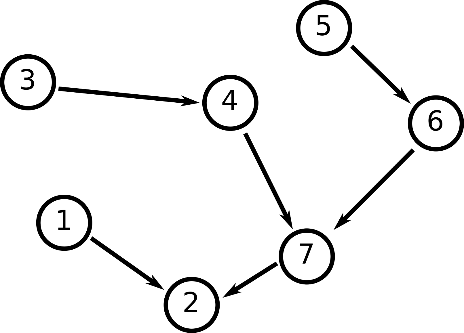
We call a network an in-tree (also called anti-arborescence [11]) rooted at state ω0∈Ω\omega_{0}\in\Omega, if for all states ω∈Ω\omega\in\Omega there is a unique directed path leading from state ω\omega towards the root ω0\omega_{0}. An example is given in Figure 5, where the root is state number 22, the distinguished state to which all the directed paths lead.
Refer to caption
Figure 5: Example of an in-tree rooted at state number 22. There is a unique directed path from each state of the tree leading to state number 22.

Further, we define

Θm​(Ω):={T⊆𝒮:T​ is an in-tree of Ω rooted in state number m }\displaystyle\Theta_{m}(\Omega):=\left\{T\subseteq\mathcal{S}\,:\,T\text{ is an in-tree of $\Omega$ rooted in state number $m$ }\right\} (25)

to be the set of all in-tree of Ω\Omega that are rooted in state number m∈{1,…,N}m\in\{1,\dotsc,N\}.

Now, suppose that the network Ω\Omega is strongly connected. Then the kernel of the corresponding generator Γ\Gamma is one-dimensional (see: section 4.3) and there is an analytical expression for it, namely:

kern ​(Γ)\displaystyle\text{kern }(\Gamma) =span ​{(∑T∈Θm​(Ω)∏(i,j)∈ℰ⁡(T)γi→j)m∈{1,…,N}}\displaystyle=\text{span }\left\{\left({{\sum\limits}}_{T\,\in\,\Theta_{m}(\Omega)}\;{{\prod\limits}}_{(i,j)\,\in\,\mathcal{E}(T)}\gamma_{i\to j}\right)_{m\in\{1,\dotsc,N\}}\right\} (26)
=span ​{(∑T∈Θ1​(Ω)∏(i,j)∈ℰ⁡(T)γi→j∑T∈ΘN​(Ω)∏(i,j)∈ℰ⁡(T)γi→j)}.\displaystyle=\text{span }\left\{\begin{pmatrix}{{\sum\limits}}_{T\,\in\,\Theta_{1}(\Omega)}\;{{\prod\limits}}_{(i,j)\,\in\,\mathcal{E}(T)}\gamma_{i\to j}\\ \\ \vdots\\ \\ {{\sum\limits}}_{T\,\in\,\Theta_{N}(\Omega)}\;{{\prod\limits}}_{(i,j)\,\in\,\mathcal{E}(T)}\gamma_{i\to j}\end{pmatrix}\right\}.

For the kk-th component of that vector you consider an in-tree TT spanning over the whole network Ω\Omega rooted in state number kk and multiply the rates of all edges ℰ⁡(T)\mathcal{E}(T) of TT. Then you sum over all such in-trees which are rooted in state number kk.
This is done for all component k∈{1,…,N}k\in\{1,\dots,N\} that is, for every state number. An illustration of this procedure can be seen in Figure 6.

(a)
Refer to caption
(b) In-tree rooted in 11
Refer to caption
(c) In-tree rooted in 33
Refer to caption
(d) First in-tree rooted in 22
Refer to caption
(e) Second in-tree rooted in 22
Refer to caption
Figure 6: Example of a strongly connected network (Figure 6(a)) together with the corresponding in-trees rooted in states number 11 (Figure 6(b)) and 33 (Figure 6(c)), and the two in-trees rooted in state number 22 (Figure 6(d) and 6(e)). The kernel of Γ\Gamma is the span of a vector whose ii-th component is the sum over all in-trees rooted in state number ii of the product of the rates of all edges that constitute that particular in-tree. In this example we have:
kern ​(Γ)=span ​{(γ3→2⋅γ2→1γ1→2⋅γ3→2+γ1→3⋅γ3→2γ2→1⋅γ1→3)}\text{kern }(\Gamma)=\text{span }\left\{\begin{pmatrix}\color[rgb]{0,0.5156,0.8008}\gamma_{3\to 2}\cdot\gamma_{2\to 1}\\ \color[rgb]{0.9023,0,0.1016}\gamma_{1\to 2}\cdot\gamma_{3\to 2}+\gamma_{1\to 3}\cdot\gamma_{3\to 2}\\ \color[rgb]{0.5,0.2695,0.5938}\gamma_{2\to 1}\cdot\gamma_{1\to 3}\end{pmatrix}\right\}.

A detailed proof for this theorem can be found in [12, 13]. The original statement was first formulated in 1948 by Tutte [14] .

It is possible to find all in-trees in 𝒪⁡(N+|ℰ|+|ℰ|⋅n)\mathcal{O}\left(N+|\mathcal{E}|+|\mathcal{E}|\cdot n\right) number of steps [11], where NN is the number of states, |ℰ||\mathcal{E}| the number of edges and nn the number of minimal absorbing sets.

As a special case, we consider the the microcanonical ensemble of statistical physics [2] where the rates for a transition and the corresponding reverse transition are identical, γi→j=γj→i\gamma_{i\to j}=\gamma_{j\to i} for all i,j∈{1,…,N}i,j\in\{1,\dots,N\}. From equation (26) follows that the stationary probability for each state is the same, i.e. 𝐩∞=1|Ω|​(1,…,1)T\mathbf{p}_{\infty}=\frac{1}{|\Omega|}(1,\dotsc,1)^{T}: For every in-tree rooted at a state i∈Ωi\in\Omega, it is possible to construct an in-tree rooted at any other state j∈Ωj\in\Omega by inverting the direction of the transitions. The overall product ∏OPEN(i,j)∈ℰ⁡(T))γi→j\prod\limits_{(i,j)\,\in\,\mathcal{E}(T))}\gamma_{i\to j} stays the same since the rates for forward and backward transitions are symmetric as is the number of in-trees for each state.

References

  • [1] N. G. Van Kampen, Stochastic processes in physics and chemistry, vol. 1. Elsevier, 1992.
  • [2] J. Honerkamp, Statistical physics: an advanced approach with applications. Springer Science & Business Media, 2012.
  • [3] H. Spohn, “An algebraic condition for the approach to equilibrium of an open n-level system,” Letters in Mathematical Physics, vol. 2, no. 1, pp. 33–38, 1977.
  • [4] P. Brémaud, Markov chains: Gibbs fields, Monte Carlo simulation, and queues, vol. 31. Springer Science & Business Media, 2013.
  • [5] N. Privault, “Understanding markov chains,” Examples and Applications, Publisher Springer-Verlag Singapore, 2013.
  • [6] R. Douc, E. Moulines, P. Priouret, and P. Soulier, Markov chains. Springer, 2018.
  • [7] J. Schnakenberg, “Network theory of microscopic and macroscopic behavior of master equation systems,” Reviews of Modern physics, vol. 48, no. 4, p. 571, 1976.
  • [8] A. Jamiolkowski and P. Staszewski, “Master equations with a unique stationary state,” Open Systems & Information Dynamics, vol. 1, no. 2, pp. 259–268, 1992.
  • [9] B. Huppert and W. Willems, Lineare Algebra, vol. 2006. Springer, 2006.
  • [10] R. A. Horn and C. R. Johnson, Matrix analysis. Cambridge university press, 2012.
  • [11] H. N. Gabow and E. W. Myers, “Finding all spanning trees of directed and undirected graphs,” SIAM Journal on Computing, vol. 7, no. 3, pp. 280–287, 1978.
  • [12] I. Mirzaev and J. Gunawardena, “Laplacian dynamics on general graphs,” Bulletin of mathematical biology, vol. 75, no. 11, pp. 2118–2149, 2013.
  • [13] S. Chaiken and D. J. Kleitman, “Matrix tree theorems,” Journal of combinatorial theory, Series A, vol. 24, no. 3, pp. 377–381, 1978.
  • [14] W. Tutte, “The dissection of equilateral triangles into equilateral triangles,” in Mathematical Proceedings of the Cambridge Philosophical Society, vol. 44, pp. 463–482, Cambridge University Press, 1948.