The final twist:
A model of gravitational waves from precessing black-hole binaries through merger and ringdown
Abstract
We present PhenomPNR, a frequency-domain phenomenological model of the gravitational-wave (GW) signal from binary-black-hole mergers that is tuned to numerical relativity (NR) simulations of precessing binaries. In many current waveform models, e.g., the “Phenom” and “EOBNR” families that have been used extensively to analyse LIGO-Virgo GW observations, analytic approximations are used to add precession effects to models of non-precessing (aligned-spin) binaries, and it is only the aligned-spin models that are fully tuned to NR results. In PhenomPNR we incorporate precesing-binary NR results in two ways: (i) we produce the first NR-tuned model of the signal-based precession dynamics through merger and ringdown, and (ii) we extend a previous aligned-spin model, PhenomD, to include the effects of misaligned spins on the signal in the co-precessing frame. The NR calibration has been performed on 40 simulations of binaries with mass ratios between 1:1 and 1:8, where the larger black hole has a dimensionless spin magnitude of 0.4 or 0.8, and we choose five angles of spin misalignment with the orbital angular momentum. PhenomPNR has a typical mismatch accuracy within 0.1% up to mass-ratio 1:4, and within 1% up to mass-ratio 1:8.
I Introduction
Binary black hole (BBH) mergers are the primary source of gravitational waves observable with current ground-based detectors Aasi et al. 2015; Acernese et al. 2015; of the 51 detections published by the LIGO-Virgo collaborations, 48 were confirmed as BBH Abbott et al. 2019; Nitz et al. 2020; Zackay et al. 2019; Venumadhav et al. 2020; Abbott et al. 2020a. Measurements of each binary’s properties — the black-hole (BH) masses and spins, and the location of the binary — rely in part on models of the signal predicted by general relativity. Model development is an active research area, with the aim that the measurement uncertainties due to model errors, approximations, and incomplete physics are smaller than statistical errors arising from the strength of the signal above the detector noise, or parameter degeneracies. Models are informed by analytic approximations for the inspiral of the two BHs and ringdown of the final BH, and NR solutions of Einstein’s equations for the late inspiral, merger and ringdown. One key physical effect is the precession of the binary’s orbital plane due predominantly to spin-orbit effects, but the two waveform families most commonly used for LIGO-Virgo parameter estimates, “Phenom” Husa et al. 2016; Khan et al. 2016; Hannam et al. 2014; London et al. 2018; Khan et al. 2019; Khan et al. 2020; Pratten et al. 2020a; García-Quirós et al. 2020; Pratten et al. 2020b; Thompson et al. 2020; Estellés et al. 2020a; Estellés et al. 2020b and “EOBNR” Taracchini et al. 2012; Pan et al. 2014; Taracchini et al. 2014; Bohé et al. 2017; Cotesta et al. 2018; Ossokine et al. 2020; Matas et al. 2020, have not been tuned to NR simulations of precessing binaries. Instead, precession effects during the strongest part of the signal have been estimated using simple approximations. These were likely sufficient for observations to date, but, given that they do not capture several physical features of the merger signal (e.g., Ref. Ramos-Buades et al. 2020, plus other effects that we will describe in this paper) more accurate models will ultimately be required.
Here we present the first Phenom model where merger-ringdown precession effects are explicitly tuned to NR simulations. We show that this model is in general significantly more accurate than previous models, particularly for binaries with large mass ratios, high spins, and a large spin misalignment.
A BBH system following non-eccentric inspiral is defined by the BH masses, and (we choose ), and the BH spin-angular-momentum vectors and . As is standard, we choose the alternative parameterisation into total mass, , symmetric mass ratio , and the dimensionless spins , where respects the Kerr limit. It is also convenient to decompose the spins into their components parallel and perpendicular to the direction of the Newtonian orbital angular momentum, , i.e., the magnitudes of the spins parallel to are , and the components that lie in the orbital plane are .
If the spins are parallel to the orbital angular momentum, i.e., , then the orientation of the binary’s orbital plane, and the directions of the spin and orbital angular momenta, are all fixed. Waveforms from these aligned-spin, or non-precessing, binaries, have been modelled with a combination of post-Newtonian (PN) and effective-one-body (EOB) results to describe the insipiral, and NR results to model the late inspiral, merger and ringdown, to produce Phenom and EOBNR waveform models Husa et al. 2016; Khan et al. 2016; Pratten et al. 2020a; García-Quirós et al. 2020; Estellés et al. 2020a; Estellés et al. 2020b; Taracchini et al. 2012; Bohé et al. 2017. Surrogate models of non-precessing systems have also been constructed purely from NR waveforms, and also from PN-NR hybrids Blackman et al. 2017a; Varma et al. 2019a.
When , the binary precesses. In most cases the binary undergoes simple precession Apostolatos et al. 1994; Kidder 1995, where the orbital angular momentum and spins precess around the binary’s total angular momentum, which points in an approximately fixed direction. Precession modulates the amplitude and phase of the gravitational-wave signal, and leads to a significantly more complicated signal than in non-precessing configurations. However, if we transform to a non-inertial co-precessing frame that tracks the precession, then the signal recovers, to a good approximation, the simple form of a non-precessing signal Schmidt et al. 2011, and, indeed, during the inspiral the co-precessing-frame waveform is approximately the signal from the corresponding non-precessing binary defined by setting Schmidt et al. 2012.
This observation has been used to construct current Phenom and EOBNR waveform models, by using a non-precessing model as a proxy for the precessing-binary waveform in the co-precessing frame, and then transforming this to the inertial frame via an independent model for the precession dynamics Hannam et al. 2014; Khan et al. 2019; Khan et al. 2020; Pratten et al. 2020b; Pan et al. 2014; Taracchini et al. 2014; Ossokine et al. 2020. Although some NR information from precessing-binary simulations has been used to model the final state Ossokine et al. 2020, the precession effects have not been tuned to NR waveforms, and neither have in-plane-spin contributions to the co-precessing-frame signal. In addition to these models, surrogate models of precessing binaries have been constructed using NR waveforms that cover roughly 20 orbits before merger Blackman et al. 2017a; Blackman et al. 2017b; Varma et al. 2019b. This puts an explicit limit on their applicability to comparatively short signals, i.e., from high-mass binaries with near-equal masses.
The current work extends the Phenom approach, the development of which has proceeded in order of the most measurable physical effects. The most clearly measurable binary parameters are the chirp mass, , for low-mass binaries where the detectable signal is dominated by the inspiral, and the total mass for high-mass binaries where most of the detectable signal power is in the late inspiral, merger and ringdown. Hence the first Phenom model considered non-spinning binaries Ajith et al. 2007; Ajith et al. 2008. The next most significant effect is due to a mass-weighted combination of the aligned-spin components, and the next set of Phenom models treated aligned-spin systems and were tuned to NR simulations that were parametrised by a single effective spin Ajith et al. 2011; Santamaria et al. 2010; Husa et al. 2016; Khan et al. 2016. All of these models considered only the dominant contribution to the signal, which is from the multipole moments. Subdominant multipoles become stronger as the mass ratio is increased, and these were first included through an approximate mapping of the dominant multipole London et al. 2018, and more recently with full tuning to NR simulations García-Quirós et al. 2020. Individual black-hole spins are unlikely to be measurable for detections with a signal-to-noise ratio (SNR) of less than 100 Pürrer et al. 2016, but a handful of such detections are likely when the LIGO and Virgo detectors reach design sensitivity in the next few years Abbott et al. 2020b, and the latest aligned-spin Phenom models include NR tuning to unequal-spin NR simulations Pratten et al. 2020b. The Phenom approach has been predominantly used to produce frequency-domain models, but has recently also been applied in the time domain Estellés et al. 2020a; Estellés et al. 2020b.
Precession effects are typically difficult to measure Fairhurst et al. 2020, and indeed have not yet been definitively observed in any single observation Abbott et al. 2019; Abbott et al. 2020a. The dominant precession effects follow the phenomenology of single-spin systems, and thus the first precessing Phenom models Hannam et al. 2014 used a single-spin PN model to estimate the effects of precession. More recent models have included two-spin effects Khan et al. 2019; Khan et al. 2020; Pratten et al. 2020b; Estellés et al. 2021, but, once again, individual spin measurements will require SNRs of at least 100, and in most cases likely much higher Khan et al. 2020. As such, the first priority for an NR-tuned precession model is the single-spin parameter space. Our new PhenomPNR model is tuned to NR simulations that cover mass ratios from equal-mass to 1:8 (). The larger black hole has a spin magnitude up to , and, as motivated by the preceding discussion, the smaller black hole has no spin. This is the widest systematic coverage of the mass-ratio–spin parameter space to date Fauchon-Jones et al. 2021.
I.1 Model approximations, and motivation for a new model
Previous Phenom and EOBNR models make use of several approximations. In this section we discuss each of these, and illustrate why we remove some of them in our new model, and the effect this has on the waveforms.
One set of approximations applies to the waveforms in the co-precessing frame.
First, as described above, during the inspiral the co-precessing-frame waveform is approximated by an equivalent non-precessing-binary waveform, . In the most recent EOBNR model, SEOBNRv4PHM Ossokine et al. 2020, the EOB equations of motion are solved for the full precessing system from a chosen starting frequency, and then the approximate co-precessing-frame waveform is constructed by now solving the non-precessing PN equations of motion, but with time-varying taken from the earlier precessing-binary solution. In the Phenom models, is defined by the aligned-spin components of the initial spin configuration, so are constant. In both families of models, contributions to the waveform multipole moment amplitudes are ignored.
Second, the mapping to an equivalent aligned-spin system breaks down at merger. This was already noted in the original presentation of the aligned-spin mapping Schmidt et al. 2012, and is also discussed in Refs. Pekowsky et al. 2013; Ramos-Buades et al. 2020. One reason is that the spin of the final black hole (and therefore the ringdown frequency and damping time) will be different to that in the non-precessing case; to first approximation, we must include the contribution from the in-plane spins, , to the spin of the final BH. In the Phenom models, the merger-ringdown part of the aligned-spin waveform is modified by using this in-plane spin contribution to estimate a modified final spin, and hence complex ringdown frequency Hannam et al. 2014; Khan et al. 2019; Khan et al. 2020; Pratten et al. 2020b; the recent PhenomXP model Pratten et al. 2020b provides a number of optional methods to achieve this. In the EOBNR models, the inspiral construction ends at the light ring Bohé et al. 2017, and ringdown modes are attached, and in the most recent SEOBNRv4PHM model Ossokine et al. 2020 these are based on an NR-tuned final spin fit Hofmann et al. 2016.
In PhenomPNR, we retain the mapping to an equivalent aligned-spin system during the early inspiral, but we introduce the key improvement that in the late inspiral, merger and ringdown we explicitly tune the model to NR waveforms in the co-precessing frame. Rather than model the final mass and spin and use those to estimate the complex ringdown frequency via perturbation theory, we also explicitly model the ringdown frequencies from NR waveforms in the co-precessing frame. As discussed in Sec. IX, this is necessary because the ringdown frequency in the co-precessing frame is shifted with respect to that in the inertial frame.
This issue is illustrated in Fig. 1. The top panel shows the frequency-domain co-precessing-frame phase derivative for one of our NR simulations, with mass-ratio , large-black-hole spin , and spin mis-aligned with the orbital angular momentum by . The figure also shows the results from the earlier PhenomPv3 model. In the inspiral we see a clear difference between the NR and PhenomPv3 results that is largest at low frequencies. The middle panel shows a second case, this time with a larger misalignment angle of . The location of the minimum can be approximately identified as the ringdown frequency, and we see that there is a clear shift between the ringdown frequency in the inertial frame (as used in PhenomPv3), and the effective ringdown frequency of the NR waveform in the co-precessing frame. This shift is also apparent in the bottom panel, which shows the amplitude in the co-precessing frame. PhenomPNR fixes this problem; see, in particular, Sec. V.
A second set of assumptions apply to the precession.
In previous models the inertial-frame waveform was constructed via a time- or frequency-dependent rotation of , using the precession angles relative to the Newtonian orbital angular momentum, i.e., the normal to the binary’s orbital plane. This produces the correct inertial-frame multipoles only in the quadrupole approximation. In order to tune the precession angles to NR results, we need a consistent choice of co-precessing frame that can be applied both to PN and NR data. For PhenomPNR we choose the quadrupole-aligned (QA) frame Schmidt et al. 2011; O’Shaughnessy et al. 2011; Boyle et al. 2011, which identifies the direction of maximum GW emission. In time-domain waveforms, the direction of maximum emission differs depending on whether it was defined using GW strain, , the Bondi news function, , or the Weyl scalar, ; and all three differ from the direction of Schmidt et al. 2011; Ochsner and O’Shaughnessy 2012; Boyle et al. 2014; Hamilton and Hannam 2018. (The direction of also depends on whether we use a Newtonian or post-Newtonian estimate.) However, we perform our modelling in the frequency domain, where the QA direction is independent of the choice of or . We explain this further in Sec. III, where we also describe in detail how we calculate the QA frame from the multipoles of NR simulations, and in Sec. VI.2 we discuss the QA frame for PN waveforms. We expect that the latter results would also allow the construction of more physically accurate EOBNR waveforms.
In most previous Phenom models, the precession angles were estimated entirely from PN theory. These angles will not be valid through merger, but as a simple approximation, they were used throughout the entire waveform. This approximation was justified by the observation that the PN angles behave smoothly to arbitrarily high frequencies, and the model gives reasonable agreement to NR waveforms Hannam et al. 2014; Khan et al. 2019; Khan et al. 2020; Pratten et al. 2020b. However, in more extreme parts of parameter space (high mass ratios and large in-plane spins), the inaccuracy of this approximation will become more serious. In EOBNR models, the inspiral precession dynamics are provided from the solution of the EOB equations of motion, and in the SEOBNRv4PHM model the precession angles are extended through merger and ringdown using an approximation based on the quantitative behaviour of NR simulations; the time-domain Phenom model, PhenomTPHM, employs a similar approach Estellés et al. 2020a.
Fig. 2 shows the precession angles for a configuration with . The figure shows both the NR results, and the multi-scale analysis (MSA) angles Chatziioannou et al. 2017 used in the PhenomPv3 and PhenomXP models. We see that at high frequencies that correspond to the merger and ringdown, the MSA estimates fail to capture the phenomenology of the NR data. The angles and both exhibit a “dip” or “bump”, reminiscent of the dip in the phase derivative in Fig. 1, which is absent in the MSA estimates. The NR opening angle drops to close to zero at merger, as we might expect as the two-body inspiral motion terminates and we are left with only a single perturbed black hole. This feature cannot be captured by the MSA expressions, which simply extend the inspiral behaviour to higher frequencies. We also find that the NR does not relax to zero, but to some non-zero value, which, if it does decay, typically does so very slowly. (There have been approximate estimates of this asymptotic decay using a toy ringdown model O’Shaughnessy et al. 2013; Marsat and Baker 2018; Estellés et al. 2020a, which we discuss and clarify in Sec. IX.) These features must also be modelled.
Finally, we see that at lower frequencies, the MSA and agree well with the NR results. However, although we expect the MSA and NR to also agree at sufficiently low frequencies, they do not agree over the frequency range of our NR data, and would likely require NR simulations that are many times longer. This discrepancy is due to the modelling inconsistency discussed earlier: the two estimates are of different quantities. The MSA is the orientation of the orbital plane, while the NR is the orientation of the QA direction of the signal, and these are not in general the same. We show how to significantly reduce this discrepancy in Sec. VI.2. (The high-frequency oscillations in the NR are due to a combination of numerical noise and Fourier-transform artifacts. All of our NR results show similar oscillations, with varying amplitude and frequency, but in these single-spin cases we will model only a smooth trend through the data, which we expect to represent their relevant physical features.)
The bulk of the results in this paper present a merger-ringdown model for the co-precessing-frame waveforms (PhenomDCP) and a separate model for the precession angles (PhenomAngles). Both modes are tuned to our NR data and capture all of the features described here. We then produce a complete inspiral-merger-ringdown model (PhenomPNR) by connecting our merger-ringdown models to inspiral results.
There are two remaining assumptions that were made in previous models, which we retain in our new model.
Non-precessing-binary waveforms satisfy a symmetry between the and multipoles that is broken in precessing binaries Bruegmann et al. 2008a; Ramos-Buades et al. 2020; Kalaghatgi and Hannam 2020. The “twisting-up” construction used by the Phenom and EOBNR models neglects these asymmetries. Although asymmetries may need to be included in models to allow accurate spin measurements in some GW observations Kalaghatgi and Hannam 2020, in the current PhenomPNR model we retain the approximation that the asymmetries in the multipole moments are zero.
Current Phenom and EOBNR models also assume that the direction of the total angular momentum remains fixed. Although the total angular momentum direction changes little through inspiral, there is some change due to the loss of angular momentum through GW emission. In PhenomPNR we explicitly transform the NR waveforms to a frame where remains fixed along the -axis, and use those waveforms as the basis of the model. In this sense the fixed- approximation is retained in PhenomPNR and remains valid over the parameter space used to construct the model, which is further discussed in Sec. XI.5.
This paper is organised as follows. In Sec. II we present our NR waveforms. In Sec. III we process the raw NR waveforms to produce the frequency-domain co-precessing-frame waveforms and precession angles that we wish to model. Since we limit the NR tuning to single-spin binaries, in Sec. IV we specify our procedure to map generic two-spin systems to approximately equivalent single-spin configurations. With all of these pieces in place, in Sec. V we present our co-precessing-frame model, PhenomDCP, in Sec. VI our treatment of the precession angles during inspiral, and in Sec. VII our merger-ringdown angle model, PhenomAngles. All of these ingredients are put together into a full inspiral-merger-ringdown model in Sec. VIII. Having modelled precessing-binary waveforms, we discuss their physical features in more detail in Sec. IX, and evaluate their accuracy in Sec. XI.
In all of the discussion of NR and PN results, and in all modelling work, we use geometric units, . We also choose , although we retain “” in plot labels, to make clear that we are dealing with dimensionless quantities. Physical masses will only be used in Sec. XI, where we study the performance of models with respect to a specific detector noise curve. All of the earlier waveform models used to generate results in this work were called from the software package LALsuite LIGO Scientific Collaboration 2018. The specific model names are IMRPhenomD for PhenomD Husa et al. 2016; Khan et al. 2016, IMRPhenomXAS for PhenomXAS Pratten et al. 2020a, IMRPhenomPv3 for PhenomPv3 Khan et al. 2019, IMRPhenomXP for PhenomXP Pratten et al. 2020b, SEOBNRv4P for SEOBNRv4P Ossokine et al. 2020, and NRSur7dq4 for NRSur7dq4 Varma et al. 2019b.
II Numerical Relativity waveforms
In producing the first precessing-binary model tuned to NR waveforms, we wish to capture the dominant precession effects first. This can be achieved with single-spin systems, i.e., only one of the black holes is spinning, since two-spin effects typically produce only small modulations of the underlying simple precession Buonanno et al. 2004; Schmidt et al. 2015. We therefore consider single-spin systems that obey simple precession, and the NR catalogue used to tune the model contains single-spin configurations where the spin is placed on the larger black hole and neglects two-spin configurations and the impact of the azimuthal spin angle. This reduces the binary parameter space from seven dimensions (mass ratio, plus the vector components of each black-hole spin), to three dimensions: the symmetric mass ratio, , the magnitude of the spin on the larger black hole, , and the angle between the spin and the orbital angular momentum of the system, . It is important to note that these are all defined as part of the initial data of the simulations, since undergoes small oscillations about some mean value during the inspiral.
We wish our model to extend to the highest mass ratios feasible with current NR simulations. The earlier tuned non-precessing model PhenomD Husa et al. 2016; Khan et al. 2016 was based on a catalogue containing systems up to mass ratio , or . NR simulations at are extremely computationally expensive, and since the mass-ratio of observations is heavily skewed towards comparable masses Abbott et al. 2019; Abbott et al. 2020a, for the current model we restrict to . We note, however, that one recent GW observation, GW190814, was measured with a mass ratio of Abbott et al. 2020c, and therefore extending our model to higher mass ratios is an urgent requirement for future work.
In order to confidently capture the dependence of precession effects on mass ratio, we produced simulations at four different mass ratios, approximately equally spaced in symmetric mass ratio . Similarly, we chose four equally spaced spin magnitudes . We already have aligned and anti-aligned waveforms in this range of mass ratios and spin magnitudes, and for non-aligned-spin configurations we chose five equally spaced values for the spin angle, , excluding and .
The model is tuned to a subset of this catalogue of 80 waveforms, which was produced using the BAM code Bruegmann et al. 2008b. The complete catalogue contains simulations with , (or ), and . For tuning we used the 40 waveforms with and 0.8. We expect the dependence of the precession effects on spin magnitude to be approximately linear, so this is not anticipated to significantly degrade the accuracy of the tuned part of the model; and this is borne out in validation of the model against the remaining waveforms in the catalogue, plus 27 waveforms from the SXS and Maya catalogues Boyle et al. 2019; SXS; Jani et al. 2016; GAT.
Since our goal is a frequency-domain model, we would like NR waveforms that all cover a similar frequency range. The majority of the waveforms start at a frequency of . However, some of the higher mass ratio configurations have a higher starting frequency in order to ensure the binary merged in a reasonable time to allow sufficient accuracy. The highest starting frequencies occur for configurations with a large spin magnitude where the spin is closest to being aligned with the orbital angular momentum, due to the hang-up effect Campanelli et al. 2006. The highest starting frequency is , for the configuration. We find that these starting frequencies are in general sufficient to match smoothly to PN results. We will see in Sec. XI.4 that there are a few cases for which we would prefer NR waveforms with lower starting frequencies, but these are actually configurations with large spins and large opening angle, e.g., . Having identified specific issues with these more challenging regions of parameter space, we will be able to focus on them in detail in future iterations of our model.
More details on the production of the NR catalogue, and error analysis of the waveforms, will be given in Ref. Fauchon-Jones et al. 2021. The greatest sources of error in these numerical waveforms are the finite resolution at which we performed the simulations and the finite distance from the source at which we extracted the GW data. We consider the mismatch (as defined in Sec. XI.1) to be the most useful uncertainty estimate for our purposes. We make a conservative estimate of the mismatch uncertainty between the waveforms in this NR catalogue and the theoretical ‘analytical’ solution of . For the shorter waveforms in the catalogue, particularly the and cases, the mismatch was found to be . As we will see when validating against independent NR data sets (e.g., those from the SXS catalogue, where the finite-extraction-radius error is minimal), the errors in our model are often an order of magnitude lower than our upper bound, and, where they are comparable or higher, the accuracy limits due to the modelling procedure are likely the dominant source of error.
For each NR simulation, spin weight spherical harmonic multipole moment data are stored for the radiative Weyl scalar,
| (1) |
where denotes complex conjugation. The depend on the choice of decomposition frame, and we provide the details of our frame choice in Sec. III. Each time series contains multipole moment data for inspiral, merger and ringdown.
In addition, spurious (“junk”) radiation, due to imperfect initial data Cook and York 1990, is windowed away, using a window function that increases from zero to one over the duration of three gravitational wavelengths. It is found that when windowing over more than two wavelengths the choice of (smooth) window function has no significant effect on our modelling results. For simplicity, a standard Hann window is used Oppenheim et al. 1999. The window starts at the first peak in the real part of such that the following peak is less than or equal to the largest distance between peaks in the time series. This most often results in less than 200 of contaminated inspiral data being tapered away. The window is applied equally to the real and imaginary parts of for all multipoles. Similarly, post-ringdown data are windowed such that the Hann window turns off to the right between the point where the exponential decay drops below the noise floor, as defined by fitting a constant value to the very end of the timeseries. The time domain data are also zero-padded to the right such that the frequency domain step size, in geometric units, is less than .
The result of the inspiral and post-ringdown windows is the reduction of frequency-domain power that is broadband and unphysical. The result of zero-padding is to enforce that frequency domain features are consistently resolved.
III Waveform frames, conventions and approximations
We wish to model the dominant multipoles of the BBH signal. The multipoles depend on the choice of reference frame, and we attempt to choose a frame that simplifies the modelling. In this section we present the reference frame in which we construct our model, and several additional simplifications that we make to the data.
If we have a set of spin-weighted spherical-harmonic multipoles , and rotate the coordinate system through the Euler angles , then the multipoles in the new frame, , are given by,
| (2) |
where are the Wigner d-matrices Wigner 1959; Bruegmann et al. 2008b.
We apply these rotations twice to our data.
First, we retain the approximation that has been used in all Phenom and EOBNR models to date, that the direction of the total angular momentum, , is fixed. This convention amounts to a minor modification of the NR data, whose radiative varies by at most from its initial direction. To impose the fixed- convention we need to know at all times in the original simulation. At the beginning of the simulation , which can be calculated analytically from Bowen-York initial data Bowen and York 1980. The angular momentum flux can be calculated from the multipole moments, e.g., Ref. Ruiz et al. 2008, and integrating this specifies the time evolution of . As a consistency check, we compare at the end of the simulation with the estimate of the final black hole’s spin calculated on the apparent horizon Campanelli et al. 2007, and find a disagreement of at most 5% in magnitude and 3% in direction. With now in hand, we use Eq. (2) to perform a time-dependent rotation to place the signal in a frame of reference where at all times. The impact of this frame convention is well below the total error budget of the final PhenomPNR model, and is discussed in more detail in Sec. XI.5.
Second, we make another time-dependent rotation into a co-precessing frame. We choose the QA frame, which was introduced in Ref. Schmidt et al. 2011, and allows us to define a co-precessing frame using the gravitational-wave signal, which is the observable quantity we ultimately care about, rather than the orbital dynamics of the two black holes. The QA method was motivated by the observation that in the quadrupole approximation, if the orbital plane lies in the - plane, then the signal can be represented entirely by the multipoles. At any other orbital plane orientation, some signal power will be distributed to the and multipoles, therefore reducing the amplitude of the multipoles. It follows that we can always identify the orientation of the orbital plane by locating the direction with respect to which the multipoles are maximised. In a time-dependent co-precessing frame where this always holds, we can represent the entire signal using only the multipoles, and, furthermore, precession modulations of the signal amplitude and phase will be significantly reduced. In general, i.e., beyond the quadrupole approximation, this direction is only approximately equal to the normal to the orbital plane, or to a PN estimate of the direction of the orbital angular momentum Schmidt et al. 2011; Boyle et al. 2014; Hamilton and Hannam 2018. However, although it cannot be directly related to the dynamics, it does provide us with a convenient signal-based definition of a co-precessing frame that suppresses precession modulations.
In the following sections we use the method described in Appendix A to calculate the coprecessing frame. We use the Euler angles , and to describe the orientation of this direction. Equations (82)-(84) define the angles accordingly, and Fig. 3 illustrates their geometric meaning.
One potential ambiguity with the QA frame is that it differs depending on whether it is defined using the gravitational wave strain, or its time derivatives, the Bondi news or the Newman-Penrose scalar . However, this ambiguity does not exist in the frequency domain.
To see this, consider the multipoles of the gravitational-wave strain, which can be written as,
| (3) |
Our NR data satisfy , and so we can write,
| (4) |
where the new amplitude and phase are given by,
| (5) | ||||
| (6) |
where we have dropped the subscripts for brevity. We see that the distribution of power between the multipoles will in general be different for and for in the time domain, and therefore the QA angles will differ.
By contrast, in the frequency domain we have,
| (7) |
where and is the gravitational-wave frequency. Since is an overall factor in front of all of the multipoles at a given frequency, the direction that maximises both and will be the same. The QA precession angles will therefore be the same for and for . Given that the frequency-domain QA angles are independent of the choice of or strain, we consider this to be the natural regime in which to work.
Finally, we also retain the standard Phenom and EOBNR approximation that the co-precessing multipole moments of our model obey the same symmetry properties as their non-precessing counterparts. This means that we neglect to model asymmetries in the multipole moments. Although the asymmetric contributions are weak, there is some evidence that they are necessary for non-biassed measurements of precessing systems Kalaghatgi and Hannam 2020, and they are certainly necessary for measurements of out-of-plane recoil of the binary Varma et al. 2020, and we plan to model these contributions in future work.
Given that have been transformed first to the fixed- and then QA frames in the time domain, we construct the symmetric combination,
| (8) |
In Eq. (8), effects an average of the co-precessing-frame mass-quadrupoles consistent with Ref. Boyle et al. 2014. We then define a symmetrised multipole according to the non-precessing symmetry relationship , thus,
| (9) |
Together, and encapsulate all waveform information that will be retained at this stage. The QA-frame multipoles are discarded, along with the multipoles; we leave higher multipoles to future work.
The symmetrised multipoles are then rotated back into the fixed- frame. We then use these data as our starting point to transform the multipoles into the frequency domain, and then transform to the QA frame as defined in the frequency domain.
We separately produce a model (PhenomDCP) of the co-precessing-frame multipole , and another model (PhenomAngles) of the rotation angles . Given these two models, our full intertial-frame model (PhenomPNR) of the multipoles, , is given via Eq. (2),
| (10) |
IV Spin parametrisation
Our goal is to model generic non-eccentric black-hole binaries with any physically reasonable values of , , and . Given NR waveforms that cover only the single-spin parameter space, we require a mapping between generic two-spin configurations and approximately equivalent configurations where . In this section we summarise our spin parameterisation. In Sec. XI.5 we demonstrate that the resulting model agrees well with a subset of the two-spin precessing-binary NR waveforms that are currently available.
Both our co-precessing-frame model PhenomDCP and angle model PhenomAngles are tuned to the same 40 single-spin NR waveforms described in Sec. II.
In the inspiral region PhenomD is based on PN expressions and so parameterised by the masses and and dimensionless spins and of the binary. The leading-order PN spin contribution to the phase is Cutler and Flanagan 1994; Poisson and Will 1995; Ajith 2011, in which the main contribution is the symmetric spin combination Ajith et al. 2011; Santamaria et al. 2010 ,
| (11) |
As such, the NR calibrated merger-ringdown region of PhenomD is parameterised by the normalised quantity,
| (12) |
The final black hole is parameterised by the final mass and spin , which are estimated using independent fits to the NR data Husa et al. 2016.
Although PhenomD is tuned to equal-spin or single-spin NR waveforms, and is often described as a single-spin model, the use of both spins in the underlying inspiral PN phase expressions, and the two different single-spin parameterizations and in the merger-ringdown calibration, mean that the model also incorporates some two-spin effects, and indeed has been shown in some cases to describe two-spin configurations to high accuracy Kumar et al. 2016.
PhenomDCP is constructed such that PhenomD is explicitly recovered in the absence of precession. To this end, PhenomD’s phenomenological parameters, which we will generically refer to as , are modified according to,
| (13) |
where is the new phenomenological parameter to be modelled across the intrinsic parameter space and quantifies the in-plane spin component and as such gives a measure of the degree of precession in the system. In Eq. (13) it is manifestly evident that, when , PhenomDCP reduces to PhenomD. The parameter is defined as part of our treatment of the precession angles, which we will now describe.
As with previous precessing-binary Phenom models, we will also use PN results to describe the precession angles through inspiral. Ref. Chatziioannou et al. 2017; Khan et al. 2019 provide complete two-spin expressions, and as such are parameterised by the masses and and the dimensionless spins and of the binary.
Conversely, for the merger-ringdown we will construct phenomenological expressions for the angles, parameterised according to the parameters of the single-spin NR simulations, . Although the NR-calibrated merger-ringdown angle model is a model of single-spin systems, we can estimate the angles for generic two-spin systems by making an approximate mapping from two-spin systems to our single-spin angle model. Our mapping is defined as follows.
We first map the spin components to the two effective spin parameters used in previous Phenom models. For the aligned-spin components we use the combination , as defined in Eq. (11). Although is the appropriate aligned-spin parameter from PN theory, in precessing systems is a constant of the PN equations of motion without radiation reaction Racine 2008, and can be seen to vary less during inspiral than .
Following Ref. Schmidt et al. 2015, we also define the effective precession spin, , based on the leading-order PN precession dynamics,
| (14) |
where , , and . parameterises the spin parallel to the orbital angular momentum while parameterises the spin perpendicular to the orbital angular momentum, i.e., in the plane of the binary.
This definition was motivated by the observation that the vectors and rotate in the plane at different rates, and over the course of the inspiral the magnitude of their vector sum will oscillate between the sum and difference of their two magnitudes. As shown in Ref. Schmidt et al. 2015, the average value of the in-plane spin contribution to the precession dynamics can be approximated well by for mass ratios . However, at mass ratios very close to one the spins precess in the plane at approximately the same rate, and so add or cancel in the same way at all times, and does not provide an ideal single-spin mapping. (This is illustrated in more detail in Ref. Gerosa et al. 2020.) Extreme examples are the “superkick” configurations Bruegmann et al. 2008a, where the black holes are of equal mass, and and . From the symmetry of the configuration, the two spins rotate at the same rate at all times, and therefore the total in-plane spin is zero, and the system does not precess. For a superkick configuration clearly does not provide the appropriate “single-spin” mapping, which in this case should be to a system with zero in-plane spin.
To deal with such cases, we also introduce , which is constructed from the vector sum of the in-plane spin vectors at a single reference time/frequency of the waveform. In our construction these are the in-plane components of the spin vectors input to the waveform generation. We define as,
| (15) |
Given a two-spin system defined by and , we model the precession angles through the merger and ringdown by mapping to a corresponding single spin, which is placed on the larger black hole. This single spin has magnitude in the direction parallel to the orbital angular momentum and in the orbital plane, where,
| (16) | ||||
| (17) |
where . This combination of and given for is designed to provide a smooth transition between the regimes where and are most appropriate. We note that for systems with , the precession effects are weak, and so the error incurred from this approximation is small, and we expect that different choices for , or for the transition to , would have an impact on GW measurements smaller than the other approximations used in our model. (Alternative choices of single-spin mapping are suggested in Refs. Gerosa et al. 2020; Thomas et al. 2020; since we use a single-spin mapping only to connect our single-spin merger-ringdown model to a generic-spin inspiral model, we expect that there are many reasonable choices of mapping that would work equivalently well.) This expression for is also used to parameterise the in-plane spin effects in the co-precessing model, as described in Eq. (13).
The total spin magnitude and the angle between the orbital and spin angular momenta are given by
| (18) | ||||
| (19) |
These reduce to the correct values for the cases to which we tuned the model and also correctly re-weight two-spin cases and cases where the spin is predominantly on the smaller black hole.
In the -aligned frame, in which we have constructed our model, the spin placed on the larger black hole has the components
| (20) |
where and are the values of the precession angles introduced in Sec. III, here evaluated at the reference frequency.
V Co-precessing-frame model
A key assumption of most precessing signal models has been that the coprecessing multipole moments are largely devoid of precession related effects Schmidt et al. 2011; Hannam et al. 2014; Pratten et al. 2020b; Ossokine et al. 2020. This assumption is motived by the PN description of inspiral, where in-plane spin components do not impact the coprecessing waveforms’ phase, and so can be disregarded Arun et al. 2009; Kidder 1995. In this sense, most precessing signal models have used un-modified non-pressing inspiral waveforms in the coprecessing frame. Because the PN motivation is only well suited for inspiral, for the waveforms’ immediate pre-merger and merger, additional assumptions must be made Schmidt et al. 2012; Pekowsky et al. 2013; Ramos-Buades et al. 2020. For example, all previous precessing-binary Phenom models use an estimate of the precessing system’s final mass and spin to compute the remnant BH’s Quasinormal Mode (QNM) frequencies. In turn, these QNM frequencies allow the frequency-domain waveforms’ features at merger to be shifted such that they occur near physically appropriate values. In Sec. I.1 we illustrated deviations from the simplifying assumptions made in both the inspiral and merger-ringdown, and in this section we refine those assumptions by constructing a tuned coprecessing waveform model.
We introduce PhenomDCP, a model for the coprecessing gravitational wave multipole moment tuned to NR. PhenomDCP is tuned to the 40 late inspiral, merger and ringdown NR simulations discussed in Sec. II. By construction, PhenomDCP reduces to PhenomD for non-precessing BBH systems. We could have instead adapted the more recent PhenomXAS model Pratten et al. 2020a, which is tuned also to two-spin systems, but since two-spin effects are unlikely to be measurable in most observations Pürrer et al. 2016; Khan et al. 2020, and we have tuned to NR results only from single-spin precessing systems, we will leave two-spin extensions of the co-precessing-frame model to future work.
We consider PhenomDCP to be a first step towards a high accuracy coprecessing waveform model. Here we briefly review the structure of PhenomD, and how this structure is extended by PhenomDCP. Physical features of the NR waveforms and PhenomDCP are provided and discussed in detail in Sec. IX. Plots showing fits of model parameters across the space of initial binary masses and spins are provided in Appendix C.
V.1 Briefly on the structure of PhenomD
PhenomD Khan et al. 2016; Husa et al. 2016 is a phenomenological model for the frequency-domain multipole moments of gravitational waves from non-precessing BBHs. The morphology of each multipole moment is organized into three regimes: (1) inspiral, where PN theory applies, (2) intermediate, where the time domain evolution of the black holes is near merger, and (3) merger-ringdown, where the time domain evolution corresponds to the final coalescence and formation of a stationary remnant BH. PhenomD models each of these regimes with different ansätze. The coefficients of each PhenomD ansatz are functions of the initial binary’s masses and aligned spins. In PhenomDCP these coefficients are modified to depend on information about the in-plane spins.
PhenomD was calibrated to 19 NR waveforms between and . For unequal-mass systems, PhenomD is calibrated to , and for equal-mass systems is it calibrated to . In each NR simulation the black-hole spins were either equal, , or the smaller black hole was non-spinning. The calibration waveforms were hybrids of SEOBNRv2 (without NR tuning) and NR waveforms. Over the model’s calibration region, its typical deviations (mismatches) from NR are less than 1% Khan et al. 2016.
V.2 Construction of PhenomDCP
In the PhenomP models Hannam et al. 2014; Khan et al. 2019; Khan et al. 2020 PhenomD is used as an approximate co-precessing-frame model, with the ringdown frequency modified according to an estimate of the final black hole’s spin. In PhenomDCP we instead use NR waveforms to tune in-plane-spin deviations to a subset of the model coefficients. Here we briefly overview the modifications of PhenomD that result in PhenomDCP.
As in previous models, PhenomDCP assumes that in the coprecessing frame only the multipole moments are needed, and that the and strain moments are related by conjugation (Sec. III). Under these assumptions we only need model the amplitude and phase of ,
| (21) |
In Eq. (21), is the frequency domain amplitude of , is its phase, references a frequency bin in geometric units, and encapsulates the system’s initial parameters (Sec. IV),
| (22) |
where, as described in Sec. IV, the total spin consists of the aligned-spin component and the in-plane component , and for our single-spin calibration waveforms, .
Given the system’s initial parameters , PhenomDCP is defined by a series of polynomials between and phenomenological model parameters. PhenomDCP’s model parameters are based directly on those of PhenomD (Eq. 13). Specifically, PhenomDCP uses the PhenomD amplitude and phase ansatz with model parameters offset by a term proportional to . Thus, when , PhenomDCP reduces to PhenomD.
Precession effects are known to be most relevant in the late inspiral and merger-ringdown Khan et al. 2020; Hannam et al. 2014. Thus PhenomDCP is made to be equivalent to PhenomD in the early inspiral. Modified versions of PhenomD are used for the waveforms’ late-inspiral phase, merger-ringdown phase, and merger-ringdown amplitude:
| (23) |
| (24) |
| (25) |
In Eqs. (23)-(25) Greek symbols denote model parameters defined in Ref. Khan et al. 2016, and of those, primed symbols, such as , denote parameters modified for PhenomDCP. Please note that these Greek symbols should not be confused with the Euler angles that define the coprecessing frame. In Eq. (24), is an “effective ringdown frequency” that is particular to the phase. Similarly, corresponds to the ringdown decay rate. In the setting of PhenomD, and are simply refereed to as and . In Eq. (25), is an effective ringdown frequency particular to the amplitude, and is equivalent to the ringdown decay rate used in PhenomD,
| (26) |
Our notation for the effective ringdown frequencies signals that we will not assume a direct relationship between the ringdown frequencies predicted by BH perturbation theory, and those relevant for coprecessing waveforms. This point is discussed further in Sec. IX.
In constructing PhenomDCP it was found that only a subset of PhenomD’s parameters needed to be modified. These parameters are those needed to address the disconnect between PhenomD and the coprecessing frame NR data discussed in Sec. II. The modified parameters correspond to the late inspiral behavior of the frequency domain phase,
| (27) |
the merger-ringdown phase,
| (28) | ||||
| (29) | ||||
| (30) |
and the merger-ringdown amplitude,
| (31) | ||||
| (32) |
In Eqs. (23)-(26), all parameters not defined in Eqs. (27)-(32) are defined in Ref. Khan et al. 2020. Similarly, in Eqs. (27)-(32), are defined in Ref. Khan et al. 2020.
The calibration of PhenomDCP has been performed by fitting Eqs. (23)-(26) to each NR waveform in our calibration set.
This yields a collection of calibration points for each model parameter.
For each of PhenomDCP’s model parameters, these points were modeled as polynomials in using gmvpfit,
which uses multidimensional least-squares regression driven by a greedy algorithm London and Fauchon-Jones 2019; London et al. 2020.
Figures 25-26 show the behavior of the PhenomDCP model parameters as functions of symmetric mass-ratio and over the calibration space. The parameter surfaces shown in Figs. 25-26 correspond to percent root-mean-square errors of in amplitude and in phase.
Figure 4 compares evaluations of PhenomDCP to NR and PhenomPv3 for the cases discussed in Sec. I.1. The top panel of Fig. 4 highlights the effect of modifying the phase. The middle and bottom panels highlight the effect of modifying the effective ringdown frequency and damping times. We see that PhenomDCP successfully corrects for the discrepancies in the modified-PhenomD co-precessing-frame model used in PhenomPv3; see Sec. XI for quantitative accuracy results.
VI Precession angle model: inspiral
Our model of the precession angles consists of two parts. The first describes the precession during inspiral, and is based on the MSA angles presented in Ref. Chatziioannou et al. 2017, and used in previous Phenom models Khan et al. 2019; Khan et al. 2020; Pratten et al. 2020b. The second part is a phenomenological model of the precession angles during merger and ringdown, tuned to the NR waveforms presented in Sec. II. We discuss the inspiral angles in this section, the merger-ringdown angles in Sec. VII, and the combined inspiral-merger-ringdown (IMR) angle model in Sec. VIII.
VI.1 MSA angles
The precession angles in the inspiral regime are calculated using PN theory. In Ref. Chatziioannou et al. 2017; Chatziioannou et al. 2017 the authors derived a closed-form analytic approximation to the inspiral precession dynamics. To achieve this GW driven radiation-reaction was introduced into an analytic solution to the conservative precession dynamics Kesden et al. 2015 by exploiting the hierarchy of timescales in the binary inspiral problem using a mathematical technique called multiple scale analysis Klein et al. 2013; Chatziioannou et al. 2013. The hierarchy of timescales are , where , and are the orbital, precession and radiation-reaction timescales respectively. This model is a function of all 6 spin components (two -vectors for each BH) and incorporates spin-orbit and spin-spin effects to leading order in the conservative dynamics and up to 3.5PN order in the dissipative dynamics, ignoring spin-spin terms. The MSA angles are shown for an example configuration in Fig. 2. We can see that the agreement is poor for all three angles at high frequencies, which correspond to the merger and ringdown. At lower frequencies, the PN and NR values for and agree well, but for do not. As noted earlier, this is because the PN describes the inclination of the orbital plane with respect to , which differs from the inclination of the QA direction.
In the next section we apply higher-order PN information to improve the PN estimate of .
VI.2 Higher-order PN corrections to
As discussed in Sec. III, in the quadrupole approximation the maximum GW signal power is emitted perpendicular to the orbital plane, and therefore the angles that describe the precession dynamics of the orbital plane are the same as those associated with the QA frame of the GW signal Schmidt et al. 2011; O’Shaughnessy et al. 2011; Boyle et al. 2011; this motivated the original QA procedure presented in Ref. Schmidt et al. 2011. For the full signal, this identification is only approximate Schmidt et al. 2011; Ochsner and O’Shaughnessy 2012; Boyle et al. 2014; Hamilton and Hannam 2018, and we expect the approximation to be less accurate at higher frequencies. Our modelling approach is based on applying a frequency-dependent rotation to a model of the waveform in the co-precessing QA frame, and as such the rotation angles should be those associated with the signal. However, all current models Hannam et al. 2014; Pan et al. 2014; Taracchini et al. 2014; Khan et al. 2019 use the angles associated with the dynamics.
As we saw in Fig. 2, the MSA dynamics and provide a good approximation to the corresponding NR signal angles at low frequencies, but the MSA does not. Fortunately, we have access to PN signal amplitudes beyond the quadrupole approximation, and can use these to calculate a more accurate estimate of the signal . One way to do this would be to calculate a full PN waveform, e.g., from the model in Ref. Chatziioannou et al. 2017, and apply the quadrupole-alignment procedure to calculate . However, this will be much more computationally expensive than the current MSA approximant, and it is possible to obtain a sufficiently accurate result with a simpler approach.
In this calculation we will refer to the opening angle of the orbital plane with respect to as , and continue to denote the opening angle of the QA frame by .
To illustrate our approach, consider the rotation from a co-precessing signal that contains only the multipoles, , to produce a precessing-binary signal in the inertial frame. We begin in the quadrupole approximation, where the inertial frame is identified with the precession of the orbital plane, and so we use the opening angle . We will focus on only the resulting and multipoles in the inertial frame, and only the angles (since the additional phase rotation will not affect our argument). The precessing-binary signal in the inertial frame, , is now,
| (33) | |||||
| (34) | |||||
The non-precessing multipoles can be written as,
| (35) |
where and are the time/frequency-dependent amplitude and orbital phase. When is small, makes the strongest contribution to the precessing-waveform multipoles, and we see that determines the relative amplitude of and . We can isolate the term as follows,
| (36) | |||||
| (37) | |||||
| (38) |
From these we can readily calculate that the inclination is
| (39) |
At leading (quadrupole) order, is the precession angle .
If we now use higher-order PN amplitude expressions Arun et al. 2009, then the angle that identifies the frame in which the multipoles are maximised will not necessarily be the same as the inclination angle , but the expression above will still give us an estimate of the orbit-averaged . Note that the MSA angles in Ref. Chatziioannou et al. 2017 are also orbit-averaged (i.e., nutation effects are absent), so this is a consistent treatment.
The multipole expressions in Ref. Arun et al. 2009 are given in terms of the orbital phase , the precession angles and , and the spin components. For the spin components, we make an approximate reduction to our single-spin systems as follows. The inclination of the spin from the -axis is the spin’s inclination from the orbital angular momentum vector, , minus the inclination of the orbital angular momentum from the -axis, . The azimuthal angle of the spin vector is , because, since , the --plane components of and will be in opposite directions, and so their azimuthal angles will differ by . The final result, for a given configuration, depends only on the dynamics inclination as a function of frequency; we use the MSA expression for .
In Ref. Arun et al. 2009 the amplitudes are expanded in powers of . We define , where , and so ; , , , and so,
| (40) |
If we substitute these into the PN multipole expressions for and , and then apply Eq. (39), we obtain the relatively simple expression,
| (41) |
where
| (42) | |||||
| (43) | |||||
Fig. 5 also shows the modified for the configuration. We see the PN inspiral now shows much better agreement with the NR result at low frequencies. We find similar results across the parameter space that we have considered, and therefore to calculate in our model, we use Eq. (41) in conjunction with the MSA as calculated in Refs. Chatziioannou et al. 2017; Khan et al. 2019, to construct through the inspiral. The features of the NR at higher frequencies, which are not captured at all by the PN expressions, will be explicitly modelled in Sec. VII.
VI.3 Two-spin
The MSA for a two spin system shows oscillations that become unphysically large through late inspiral and towards merger and which are not seen in the precession angles calculated for two-spin NR systems, as can be seen in Fig. 6. These oscillations also complicate connecting the inspiral expression to the single-spin-tuned merger-ringdown ansatz. We therefore taper these oscillations to recover the value and gradient of for an equivalent single-spin system at the point at which we wish to connect the inspiral and merger-ringdown parts of the model.
For a system described by two spins and we use the mapping to the appropriate single spin system defined in Sec. IV: is given by Eq. (20) and . We evaluate the PhenomPv3 expression for for both of these configurations and identify the oscillations introduced by the two-spin effects as,
| (44) |
We then apply a taper to these oscillations that ensures will tend to the single spin value and gradient at a given frequency and add the oscillations back to the single-spin function. The final two-spin expression for is then given by
| (45) |
where is the frequency at which the inspiral expression for is connected to the merger-ringdown expression defined below in Eq. (57).
Given an estimate for the dynamics , we now wish to rescale it to produce an estimate for the signal , as described in Sec. VI.2. To do this we also need an estimate of the frequency-dependent in-plane spin component, and therefore and , as required in Eqs. (40). We assume that the component of the spins parallel to the orbital angular momentum, , remains fixed. We further approximate that the frequency dependence of the magnitude of is dominated by changes to the magnitude of ,
| (46) |
where the magnitude is given by the 3PN expression for the orbital angular momentum used by PhenomPv3 to calculate and the 0-subscript denotes quantities specified at the reference frequency. As such, we may write the frequency-dependent in-plane spin component as
| (47) |
Substituting this expression for in Eq. (14) we get a value for . The quantities and are then calculated as described in Eqs. (11)– (19) and these values are used to rescale to produce , according to Eq. (41).
The effect of this treatment can be seen in Fig. 6, which shows for SXS1397 (the intrinsic properties of which are given in Tab. 2). The PN expression for the angle captures the oscillations seen at low frequency very well. However, these oscillations do not continue to high frequency and are greatly over-estimated by the full two-spin PN expression. Tapering the oscillations to the single spin value at the connection frequency resolves this issue well. For the PN expression is replaced by the merger-ringdown expression described in the following section, so the behaviour of the PN angles here are not an issue. In the rare event where the merger-ringdown contributions are not attached (see Sec. VIII.4), only the effective single-spin beta is used beyond .
VII Precession angle model: merger-ringdown
The PN expressions for the precession angles cannot be reliably extended through merger and ringdown and when compared with the NR angles do not capture the features present at high frequency, as was clear in Fig. 2. We therefore present a phenomenological description of the precession angles and in the merger-ringdown regime; the remaining angle can then be calculated via Eq. (84). We describe the functional form of the angles and produce a global fit for each of the co-efficients of the ansatz. This provides a frequency domain description of the precession angles across the parameter space.
VII.1 Functional forms of and
The morphology of the merger-ringdown part of is qualitatively very similar to that of the phase derivative, seen in Ref. Husa et al. 2016; Khan et al. 2016. shows a fall-off with a Lorentzian dip centred around what is approximately the ringdown frequency of the BBH system. This prompts the ansatz,
| (48) |
where , , and are free co-efficients.
The fitting region is based around the Lorentzian dip; it is defined to be the range , where is the frequency at which reaches its minimum, and recall that we have chosen . The global fit for within this fitting region has a root mean square error of , averaged across the 40 waveforms. Some example comparisons of the result of these fits with the NR value for are shown in Fig. 7.
During merger and ringdown, drops rapidly as the dominant emission direction relaxes to its final direction, as discussed in more detail in Sec. IX. The ansatz used to describe is therefore chosen to grow at low frequencies (as seen in the PN expressions), turnover at the correct frequency, capture the drop and finally tend asymptotically towards the constant value to which the dominant emission direction relaxes. The ansatz we chose to describe this behaviour is,
| (49) |
where , , , and are free co-efficients.
The fitting region for is centred around the inflection point in the turnover ; . The global fit for within this fitting region has a root mean square error of , averaged across the 40 waveforms. Some example comparisons of the result of these fits with the NR value for are shown in Fig. 8.
VII.2 The phenomenological co-efficients
The two ansätze given above, which describe the merger-ringdown behaviour of , Eq. (48), and , Eq. (49), have 10 free co-efficients between them. Each of these co-efficients was fit across the three-dimensional parameter space described by the symmetric mass ratio, , the dimensionless spin magnitude, , and the cosine of the angle between the orbital angular momentum and the spin angular momentum, .
The optimum value of each of the co-efficients for each waveform in the calibration set was found by fitting the relevant ansatz to the NR
data using the non-linear least-squares fitting function curve_fit from the python package Scipy Virtanen et al. 2020.
This function uses the Levenberg-Marquardt algorithm to perform the least-squares fitting. We then performed a three-dimensional fit of
each of the co-efficients using the fitting algorithm mvpolyfit London and Fauchon-Jones 2019; London et al. 2020.
This gives each of the co-efficients as a
polynomial expansion in , , . We specify the terms that appear in the expansion and the algorithm finds the co-efficients of
these terms that optimise the fit as well as a measure of how good the fit is. Since we have 40 calibration waveforms, the maximum possible
number of terms
that can appear in these expressions is 39 in order to avoid over fitting. The fits are restricted so that the highest order term in each
dimension is one less than the total number of data points in that dimension. Since the value of each of the co-efficients in the ansatz is to
some extent dependent on
the value of each of the other co-efficients, we found a global fit for each co-efficient in turn, re-fitting the ansatz to the data while
keeping fixed the co-efficients that had already been fit.
We first fitted the co-efficients that varied most smoothly across the parameter space and those for which the general behaviour across the
parameter space was already understood. For this meant we first fitted the location of the dip, , followed by the other co-efficients
in the order , and . For we fitted the value of separately as this had a clear parameter
space trend. We then fitted the co-efficients in the order , , , and since the co-efficients in the numerator were generally
better behaved than those in the denominator.
The general expression for each co-efficient is
| (50) |
where are the co-efficients in the ansatz describing and respectively and and respectively. The give the co-efficients of the polynomial expansion of the multi-dimensional fits of . This expression has a maximum of 40 terms. Not all of these terms are used in the expressions for each of the co-efficients; the co-efficient with the fewest number of terms has only 25 while that with the greatest number of terms contains 39.
The co-efficients for and vary smoothly across the parameter space, as can be seen in Figs. 27 and 28 in Appendix C respectively. The residual plots above the fit surfaces show that the global fits agree closely with the values of the co-efficients found from fitting the ansatz to each individual simulation.
VIII Full inspiral-merger-ringdown angle model
The expressions for the precession angles for the two distinct inspiral and merger-ringdown regions are connected so that the connection is smooth and the full IMR expression for the angles agrees with the NR data over the entirety of the region for which it is available. The method used to connect the two regions was different for each angle.
VIII.1 Connection method for
For , the regions are connected using an interpolating function of the form
| (51) |
defined over the frequency range . This range was chosen to be as small as possible. The lower frequency limit was chosen to be the highest frequency for which the inspiral expressions agreed with the NR data while the upper frequency limit was chosen to be the lower limit for which the fitted merger-ringdown expressions still agreed well with the NR data. Since the MSA PN expressions for the angles agree well with the NR data over most of the waveform, there is a wide range of frequency values over which the interpolation could be performed. We choose the frequency range to be defined in terms of the location of the Lorentzian dip, : and .
The co-efficients of Eq. (51) are chosen so that
- 1.
and , since there is freedom in an overall constant offset in ,
- 2.
and in order to ensure the two parts are connected continuously.
is the MSA PN expression used for in the inspiral regime. is the merger-ringdown ansatz given in Eq. (49). The co-efficients are given by
| (52) |
where and , , are the value of and its derivative at the limits of the frequency range and .
VIII.2 Connection method for
For , the agreement between the PN expression and the NR data is insufficient to employ the interpolation method described above. Even including the higher order amplitude corrections described in Sec. VI.2, the starting frequency of the NR simulations is not low enough in order to cover the region in which the PN expression closely matches the data for all cases. Instead, we employ a rescaling function that leaves the PN expression invariant at low frequencies but ensures it smoothly connects with the merger-ringdown value of at the connection frequency . This rescaling function is given by
| (53) |
which tends to one at low frequencies thus leaving the PN expression unchanged. In order to ensure the value of and its derivative match at the connection frequency, the co-efficients and are given by
| (54) | ||||
| (55) |
where the and are the value of and its derivative evaluated at the connection frequency. The subscript 1 indicates that this is the value of given by the original PN expressions while 2 indicates the values from the merger-ringdown expression.
The definition of the connection frequency depends on the morphology of the merger-ringdown ansatz for for a particular case. As can be seen in Fig. 8, in some parts of the parameter space rises gently until just before merger then turns over and drops rapidly. However, in other parts of the parameter space this turnover is much more gradual and begins at much lower frequencies. Our ansatz for captures both of these morphologies well. In cases where the turnover occurs within the fitting region, we define the connection frequency as the frequency at which the merger-ringdown part has a particular gradient . The value of this gradient varies across the parameter space. We define it to be
| (56) |
where is the gradient at the inflection point. The connection frequency is then found by expanding the gradient of the curve about the maximum as a Taylor series. We find the connection frequency is given by
| (57) |
where is the frequency at which the maximum occurs and and are the second and third derivatives of evaluated at , respectively.
In cases where the turnover is not present within the fitting region we instead define the connection frequency to be the lower frequency limit of the fitting region, thus ensuring is still falling at this frequency. In this case,
| (58) |
where is the inflection point.
VIII.3 Full IMR expressions
The expressions describing the precession angles in each of the different regions are connected using piece-wise -continuous functions.
The full IMR expression for is
| (59) |
where , and are the PN expression used to describe during inspiral, the interpolating function used to describe the late inspiral angles in the region to and the phenomenological ansatz used which has been tuned to NR to describe the merger-ringdown angles respectively.
Across the majority of the parameter space, the merger-ringdown ansatz for has a minimum immediately following the inflection point (as shown in the central panel of Fig. 10). In these cases, the full IMR expression for is
| (60) |
where is the PN expression for including the higher-order amplitude corrections discussed in Sec. VI.2, is the rescaling function applied to these expressions as outlined above, is the phenomenological ansatz which has been tuned to NR in the merger-ringdown regime, and is the constant value of to which the system settles down after merger, as discussed in Sec. IX.2. We model this quantity by the minimum value of in the merger-ringdown expression. is correspondingly given by the frequency at which the minimum occurs.
In cases where tends towards an asymptote immediately following the inflection point (which occur in some regions of parameter space beyond the fitting region), the full IMR expression for is
| (61) |
We would physically expect to be bounded by 0 and across the parameter space. In order to enforce this requirement, we pass the resulting through a windowing function given by
| (62) |
where . This function is linear with over the range to within 0.045%. This ensures that the fits for are unaffected within the calibration but that is bounded by 0 and across the whole of parameter space.
The precession angle is then calculated over the entirety of the frequency range for which the waveform is produced by enforcing the minimal rotation condition given in Eq. (84). The decision to do this rather than produce a separate model for was made as it was found that must be very accurate in order to consistently transform between an inertial frame and the co-precessing frame. The very small discrepancy between the expression for presented in Chatziioannou et al. 2017 and the numerically calculated value is sufficient to seriously degrade the model. This discrepancy is exacerbated here since we are no longer using the dynamical expression for presented in Chatziioannou et al. 2017. (We note that independently integrating Eq. (84) was also found to be more accurate in the SEOBNRPv4HM and PhenomTPHM models Ossokine et al. 2020; Estellés et al. 2020a.)
The full model of these angles is shown for two examples in very different parts of the parameter space in Fig. 9.
VIII.4 Behaviour beyond calibration region
As with any tuned model, beyond the calibration region there is no guarantee of the accuracy of the model for the angles. However, we want to ensure that they do not display pathological or obviously physically incorrect behaviour.
For there are a number of possibilities inherent in the ansatz to see either pathological or physically incorrect behaviour. We have implemented restrictions on the values taken by the co-efficients to ensure this does not occur and a visual inspection of the waveforms shows that we do not see any pathological features. We would see pathological behaviour for and physically incorrect behaviour for ( would decrease as a function of frequency) or (the dip in would have the wrong sign). As it is only a small region of parameter space in which this might happen, we enforce the conditions that and by taking the absolute value of the co-efficients with the appropriate sign. For we replace any positive values with zero. and take the wrong sign for systems with only at very small spins () or large anti-aligned spins (). For there is an additional region for around for anti-aligned spins (). does not go negative within the calibration region, though this does start to occur for .
We see pathological behaviour for . Physically incorrect behaviour starts to emerge when drops below . In order to avoid such behaviour we require and replace the fitted value of by 175 where it falls below this value. Since across the majority of the parameter space this concern only arises for very extreme configurations () where the accuracy of the model cannot be guaranteed anyway.
The morphology of the merger-ringdown ansatz of also changes in some parts of the parameter space outside the calibration region, as shown in Fig. 10. We can ensure we always employ the correct part of the expression (for which displays a drop at merger) in our model by selecting the correct inflection point. The inflection points of an expression occur at the roots of the second derivative of the expression. The second derivative of Eq. (49) takes the form
| (63) |
where , , and are functions of the fitting co-efficients , , , and . In order to find the roots of this cubic we re-write it in the form of a depressed cubic
| (64) |
where
| (65) | ||||
| (66) | ||||
| (67) |
In the case where this expression has three real roots, these are given by
| (68) |
where .
We want to be able to define a single, smoothly varying inflection point that tracks the location of the turnover in during merger across the parameter space. As the co-efficients of the cubic vary, the morphology of Eq. (49) changes, as shown in Fig. 10. For we have the morphology shown in the central panel of the figure. We therefore select the central root, which is the only one with a negative gradient. For , we have the morphology shown in the outer panels. For this morphology we need to distinguish between the two outer roots, which both have a negative gradient. This is determined by the “shift” of the roots, . In cases where
| (69) |
where the are the co-efficients given in Eq. (50), we choose the first root (as seen in the left-hand panel), otherwise we choose the final root (as seen in the right-hand panel). This condition was found to select the correct root across the entire calibration region for the model as well as most of the extended regions encompassing the validation waveforms.
In the case where we have complex roots, two of the roots will be in the complex plane while one will be on the real axis. In this case we select the only real root.
We also consider the case where and the second derivative is a quadratic. In this case we have only one root with a negative gradient, which is the desired root. Finally, we consider the case where both and . Here we have only one root which gives us the desired inflection point.
Enforcing these conditions gives us a smoothly varying value of the inflection point across the parameter space and ensures our expression for always has the correct morphology, dropping off at merger.
IX Physical features of the waveforms
In motivating, constructing and presenting the PhenomPNR model, we have observed several features of precessing-binary waveforms that deserve more detailed discussion.
IX.1 Ringdown frequency
As discussed in Sec. V, in previous Phenom models, the co-precessing-frame model consists of an aligned-spin model, with ringdown frequency and damping time adjusted according to the values predicted for the full precessing configuration. This prediction was made by using approximate NR fits for the final mass and spin, which then imply, via perturbation theory, the ringdown frequencies. This prediction of the ringdown frequency was then used in the co-precessing-frame model.
One interesting feature of this approach is that in some parts of the parameter space it leads to a discontinuity in the ringdown-frequency estimate. This arises as follows. There are two choices of ringdown frequency for a given BH spin, depending on whether the BH perturbations were generated by orbits that were prograde or retrograde with respect to the final BH spin; this can be represented as choosing either a positive or negative final spin. As an example, consider configurations with mass ratio and a spin on the larger BH of . If the spin is aligned with the orbital angular momentum, we predict that after merger the final BH will have a spin of 0.86, and a ringdown frequency of 0.1. If the large BH spin is anti-aligned to the orbital angular momentum, i.e., , then the final BH spin is , and the ringdown frequency is 0.06.
We can now ask, what happens for other values of ? In previous Phenom models, the final spin was estimated as follows. We first estimate the final spin for an equivalent aligned-spin binary, , and then calculate the vector sum of this aligned spin with the in-plane spin contribution , which, in our single-spin example above, would take the value . The final spin is then estimated as,
| (70) |
When we use this final-spin estimate to calculate the ringdown frequency, we must choose a sign. In previous Phenom models, the same sign was chosen as , but in some cases (as in the example above), this means that swaps sign at some value of , and the resulting estimate of the ringdown frequency is discontinuous. This is illustrated by the dashed line in Fig. 11 for our , series of configurations. As an estimate of the ringdown frequency in the () multipoles in the -aligned frame, this approach appears to be quite accurate, including the sharp transition from prograde to retrograde branches.
One issue with this approach is that the transformation from the co-precessing to inertial frame will introduce a shift in the GW frequency, and therefore a change in the ringdown frequency. If we apply the correct inertial-frame ringdown frequency to our co-precessing-frame model, it will be changed when the angle model is applied, and the final model will have the wrong ringdown frequency. This is what happens in previous Phenom models. We could take this shift into account when we prescribe the ringdown frequency in the co-precessing frame, but instead we simply produce a phenomenological fit to the ringdown frequency in the construction of the co-precessing-frame model PhenomDCP. This is also shown in Fig. 11, in comparison with the effective co-precessing-frame ringdown frequency that we find from the NR data.
IX.2 The collapse of through merger
During the inspiral, the angle is related to the opening angle between the total and orbital angular momenta, i.e., the opening angle of the precession cone. At merger the orbital motion ceases, and we are left with a ringing black hole, and would expect that the corresponding optimal emission direction would relax to the direction of the final black hole. However, we may also consider an alternative picture. A stationary BH does not radiate. We may perturb a non-spinning BH such that we completely determine the dominant emission direction as the perturbation rings down. Adding spin to the BH, either small or large, does not change this freedom. Thus the optimal emission direction after merger, and in particular, the final values of and , may encode information about how the remnant BH was perturbed through merger, and the relationship to is not so clear.
In Ref. O’Shaughnessy et al. 2013 an attempt was made to describe the late-time precession behaviour using results from perturbation theory. We know the general form of the ringdown signal,
| (71) |
where the are unknown constants, and are determined by the mass and spin of the final BH through perturbation theory. Given this general form, we can predict the general behaviour of the precession angles and in the ringdown regime, similar to the approximate approach followed in Sec. VI.2. Ref. O’Shaughnessy et al. 2013 note that, if we consider only the dominant modes, the QA direction precesses around with a frequency , and either falls exponentially to zero at a rate given by , or grows exponentially to , depending on the relative magnitude of the two damping times. A similar calculation was later discussed in Refs. Marsat and Baker 2018; Ossokine et al. 2020; Estellés et al. 2020a.
Several points are worth noting. (1) For much of the parameter space, although the decay of is exponential, it is nonetheless extremely slow, and on a much longer timescale than the decay of the signal amplitude. (2) We can consider non-zero and multipoles where the QA direction does not precess at all, for example all aligned-spin binaries. (3) Just as BH perturbation theory cannot tell us how much each QNM is excited Kamaretsos et al. 2012a; Kamaretsos et al. 2012b, this analysis cannot tell us the magnitude of at whatever point we wish to designate as the beginning of the ringdown regime.
We now turn to our NR data to address these points. Fig. 12 shows the late-time behaviour of NR for the and configurations, as well as approximate fits to the decay rate predicted by the ringdown toy model discussed above. In these fits the decay rate is prescribed by the toy model and only the overall amplitude is fit to the numerical data. The data are not clean enough to conclusively show that late-time follows the decay rate predicted by the toy model, but the data are certainly consistent with that model. What is worth highlighting is that the decay rate is indeed very slow; we expect to be greater than, say, 10% of its peak value, for several hundred after merger, at which point the total signal amplitude will have decayed by several orders of magnitude. In this context, our simple approximation in PhenomPNR, that late-time is constant, appears to be justified.
The other important observation is that this late-time ringdown behaviour begins after has dropped significantly through merger. This strongly suggests that ringdown begins significantly after the peak in both strain and , which is possibly at tension with recent efforts to apply BH perturbation theory at those points Giesler et al. 2019.
Although a PN treatment can approximately describe during the inspiral, and a simple ringdown analysis can describe the decay rate of during ringdown, neither can capture the rapid drop in through merger, or predict the value of at the point where the ringdown behaviour takes over. This feature, which is included in PhenomPNR, was not explicitly modelled in previous Phenom and EOBNR models; PhenomP/Pv2/Pv3/XP used the MSA angles at all frequencies, and both SEOBNRv4PHM and PhenomTP use a constant late-time value of determined by its value near merger.
IX.3 Hierarchy in the turnover frequency of the multipoles
The rapid drop in described in the previous section results in a key feature of precessing waveforms: a hierarchy in the turnover frequency of the multipoles. From Eq. (39) we can see that is approximately given by the ratio of the amplitude of the (2,2) and (2,1) multipoles. The drop in therefore implies that the amplitude of the (2,1) multipole must have decreased relative to the (2,2) multipole and so the (2,1) multipole will begin to experience ringdown decay before the (2,2) multipole. Once both multipoles are decaying exponentially (at roughly the same rate) levels off. This trend continues for all of the multipoles.
By capturing the drop in in our model, we succesfully model this hierarchy in the turnover frequency of the multipoles, as seen in the top panel of Fig. 13. This feature has not been modelled in previous precessing Phenom models, and the central panel of Fig. 13 shows the multipole hierarchy for PhenomXP, which is also the behaviour for PhenomPv3, since both use the same MSA angle model. We see that in these models each of the multipoles turn over at the same frequency. SEOBNRv4P, shown in the bottom panel, does capture this hierarchy but the amplitude of the higher order multipoles is not well modelled. This is due to modelling rather than , which typically overestimates the amplitude as discussed in Sec. VI.2.
X Time domain validation
X.1 Time domain waveform
The improvements made in modelling precessing systems presented here — both to the underlying co-precessing model and the precession angles — can also be clearly seen when inspecting the waveforms in the time domain. As can be seen in Fig. 14, PhenomPNR correctly captures the precession envelope and the phasing of the waveform through inspiral, merger and ringdown. This figure also clearly shows that the frequency-domain modelling presented here does not introduce any strange artefacts in the time domain. For comparison we also show SEOBNRv4P, a naturally time domain precessing model. The configurations shown here are for a binary with the intrinsic properties (top panel) and (bottom panel). We have plotted the optimally aligned waveform for both waveform models for a face on () binary. We particularly note the good agreement between PhenomPNR and the NR waveform after merger (the shaded region) due to accurately modelling the merger-ringdown precession angles and the effective ringdown frequency of the co-precessing waveform.
The time and phase alignment of the waveforms plotted in Fig. 14 has been performed over the same range of frequencies as were used in calculating the matches detailed in Sec. XI and quoted in the figure legend. This range is much greater than that shown in the plot so the deviations between the models and the NR seen here do not contribute as much as might naïvely be expected. We have plotted the waveform for the in-plane spin configuration and polarisation of the signal for which we get the maximum match. PhenomPNR agrees well with the NR data from inspiral through merger and ringdown, capturing both the precession envelope and the phasing of the waveform correctly.
X.2 Time domain angles
Accurately modelling the merger-ringdown features of the angles in the frequency domain has also enabled us to reproduce key features of the angles in the time domain after merger. We compared the time domain angles for four models (PhenomPv3, PhenomXP, SEOBNRv4P and PhenomPNR) with the NR angles. In order to avoid the introduction of artefacts due to unnecessary processing of the NR data, we compare against the time domain angles calculated using the cleaned and symmetrised data rather than .
The time domain angles for the frequency domain models (those belonging to the Phenom family) are calculated as follows. First we compute the multipoles from the strain multipoles in the frequency domain using . We then compute the time domain multipoles by performing the inverse Fourier transform each of the frequency domain multipoles. Finally we calculate the precession angles from the set of time domain multipoles.
For SEOBNRv4P, a time domain model, we differentiated each of the time domain multipoles twice to get from . We then calculated the precession angles using these multipoles. Since the connection between the inspiral and ringdown parts of the models for the multipole moments and the precession angles used in SEOBNRv4P is -continuous, we see a discontinuity in the time domain angles presented here as a result of the double differentiation.
The results of this comparison are shown in Figs. 15 and 16. Since PhenomPv3 and PhenomXP use the same model for the precession angles with a different co-precessing model, the time domain angles presented here agree very closely. The two most notable features in the time domain angles are the continued rise in after merger and the rapid drop in the value of . If takes a constant value it implies the precession of the optimum emission direction has stopped. As has been noted previously O’Shaughnessy et al. 2013, this is clearly not seen in the NR data. This feature of the precessional motion is captured by SEOBNRv4P and PhenomPNR but not by PhenomPv3 and PhenomXP. The rapid drop in the value of is captured accurately only by PhenomPNR, although SEOBNRv4P does show some evidence of a drop in the value of . This shows we have managed to capture the closing up of the opening angle as the angular momentum is radiated away through gravitational wave emission. The final feature to note is the amplitude of throughout inspiral is captured reasonably well by PhenomPNR whereas the other models all show a slight offset since (as previously discussed) they use the angles that describe the precessional dynamics rather than the precession of the direction of optimal emission. This can be seen more clearly at earlier times than are shown in Figs. 15 and 16 since here we chose to focus on the merger-ringdown region where data processing artefacts from the Fourier transform are stronger.
XI Model validation: Matches
We now wish to test the accuracy of our new precessing model in the context of gravitational wave signal analysis. To do this we calculate the match (using the method detailed below in Sec. XI.1) between the NR waveform and our model for a given configuration. We performed three sets of matches in order to inspect each of the components of our model individually as well as the complete final model. To assess the accuracy of the underlying co-precessing model we calculated the standard non-precessing match for a waveform containing only the (2,2)-multipole between the co-precessing model PhenomDCP and the co-precessing NR waveform. In order to assess the accuracy of the angle model itself, we model the precessing waveform by twisting up the co-precessing NR waveform with the PhenomAngles angles and match it against the corresponding -aligned NR waveform. Finally, we assessed the accuracy of the complete tuned precessing model PhenomPNR by performing the SNR-weighted match between the model and the -aligned NR waveforms, containing the multipoles. The match calculated between the NR waveform and the complete model will contain errors introduced by inaccuracies in both PhenomDCP and PhenomAngles. Since we do not aim to model asymmetries in the multipole moments in this work, our model does not capture them. We therefore perform matches testing the angle model using the symmetrised NR waveform (in both the -aligned and co-precessing frames).
XI.1 Match Definitions
The disagreement between two waveforms, a model template and an NR signal , is quantified using the standard inner product weighted by the power spectral density of the detector Cutler and Flanagan 1994, chosen for this work to be the noise spectrum of advanced LIGO at design sensitivity LSC:
| (72) |
The match is then given by the inner product between two normalised waveforms,
| (73) |
maximised over a set of template parameters described below.
Time shifts and reference phase shifts have no physical effect on the signal; a time shift corresponds only to a change in the merger time of the binary, while a change in the phase corresponds to a change in the initial orientation of the binary’s orbit. For non-precessing waveforms containing only the (2,2)-multipole, the resulting match value is independent of the inclination and polarisation of the signal, as changes to the inclination simply re-scale the overall amplitude of both the signal and template, and the polarisation is degenerate with the reference phase and therefore optimised away. When computing the match for non-precessing signals, as is done in Sec. XI.3, the maximisation done in Eq. (73) is done over time and phase shifts, .
For precessing waveforms, both the inclination and polarisation must be taken into account. First, we compute the match outlined in Eq. (73) whilst keeping the signal phase and polarisation fixed, and maximise over time shifts, reference phase and template polarisation following Ref. Harry et al. 2016. We further optimise over rotations to the in-plane spin components of the template at the reference frequency as in Ref. Pratten et al. 2020b, which effectively optimises the match over the initial precession phase , i.e., . We then follow previous efforts to quantify precessing models Schmidt et al. 2015; Khan et al. 2019; Pratten et al. 2020b and introduce an SNR-weighted match.
The SNR-weighted match is computed by averaging the match computed at each given signal phase and polarisation whilst volume-weighting with the SNR of the signal,
| (74) |
where we have summed over the values of signal phase and polarisation, and , respectively. This is done to better account for the large variation in detectability and signal strength with sky location that occurs in precessing signals.
Finally, we compute the mismatch between the signal and template for non-precessing signals as,
| (75) |
and similarly for precessing signals the SNR-weighted mismatch,
| (76) |
XI.2 Verification waveforms
We performed matches against 76 of the waveforms taken from the BAM catalogue described in Sec. II. We also considered an additional set of waveforms taken from the SXS Mroue et al. 2013; Boyle et al. 2019 and Maya catalogues Jani et al. 2016. This enabled us to test the accuracy of the model for configurations for which it was not tuned, including two-spin configurations. A summary of the waveforms taken from the BAM catalogue are given in Table 1, while the details of those taken from the SXS and Maya catalogues are in Table 2. Only the subset of waveforms taken from the BAM catalogue were used to study the accuracy of the individual components of the model; the underlying co-precessing model and the model for the precession angles. The complete set of waveforms, taken from all three catalogues, was used to test the accuracy of the full model over a range of total masses for the system.
XI.3 Matches: Accuracy of the co-precessing model
We computed the match between various models for the co-precessing waveform and the co-precessing NR waveform. We considered a system of total mass 100M⊙ and performed the match over the frequency range for which the NR data was available; from Hz to 244Hz. The value of the reference frequency for each simulation is given in Table 1. The co-precessing-frame models we consider are PhenomPv3, PhenomXP and PhenomDCP.
As can be seen from Fig. 17, the assumptions that go into producing the aligned-spin mapping used in the production of modified PhenomD and modified PhenomXAS become less accurate as both mass ratio and spin are increased. PhenomDCP performs better than both modified PhenomD and modified PhenomXAS for almost all cases, with the most noticeable improvement for the higher mass ratio, high-spin cases where we are in greatest need of a tuned co-precessing model. In the cases where PhenomDCP has a similar or slightly worse performance than either of the other two models the match is generally already comparable to the accuracy level of our input NR waveforms.
XI.4 Matches: Accuracy of the angle model
In order to test the accuracy of the angle model we constructed a set of precessing waveforms by calculating the symmetrised frequency-domain co-precessing NR waveform containing only the multipoles and “twisting” this waveform up with the modelled precession angles. We constructed two sets of precessing waveforms in this fashion; one using the model for the angles presented in this paper, and the other using the MSA angles, in order to quantify the effect of modelling the merger-ringdown behaviour of the angles. We then calculated the SNR-weighted match between these waveforms and the symmetrised NR waveforms in the -aligned frame comprising only the multipoles. As with the co-precessing matches described above, these matches were calculated at a fixed total mass M⊙ and performed over a frequency range from Hz to 244Hz (the frequency range for which the NR data was available).
In Fig. 18, we have shown the inclination average of the full precessing match for ease of presentation. We can see that the matches using the improved angle model are above 0.99 across the majority of the parameter space. The only cases for which this is not true are in the most extreme corner of the parameter space we modelled; cases with , and . In these cases we find the PN expressions used for during inspiral deviate from those calculated from the NR waveform at reasonably low frequencies. In the case of this is before the start of the NR waveform, as shown in Fig. 19. Improving the model for these cases would require a model for the intermediate region between where the PN expression ceases to be accurate and where the current model begins, which may require longer NR waveforms to be produced. Additionally, we expect that modelling this intermediate region will improve matches for several other cases as well, where the PN expressions for the angles deviate from what we see in the NR data at lower frequencies than are covered by our current merger-ringdown model for the angles. Nonetheless, in all cases we see significant improvement over the previous model.
The best matches are seen in the least extreme part of parameter space; namely for low mass ratio systems. This is the region of parameter space where existing models for the angles already perform reasonably well. The biggest improvement in the matches as a result of the improved model for the angles is seen at higher mass ratios, particularly for larger .
For a selection of these cases we show the mismatch as a function of in Fig. 20. The figure shows both the SNR-weighted average, and the range of mismatches with respect to signal polarisation and phase. We see that the mismatches against symmetrised NR waveforms are approximately symmetric about . The MSA angles generally give the worst SNR-weighted average mismatch for systems with , although this is not always the case, and the variations with respect to different choices of polarisation and phase are often larger than those with respect to inclination. This mismatch then typically improves as it approaches systems, with a slight increase for systems at exactly in most cases. In contrast, the SNR-weighted average mismatches involving the new angle model show one of two main behaviours with respect to inclination: the first gives the lowest mismatches for systems with with a marked degradation towards , while the second shows approximately constant values for the mismatch with respect to inclination, with a possible slight improvement for systems with . However, we do not observe any clear pattern in how these two trends manifest themselves across the parameter space. The most important result to note is that in comparing the new angle model with the MSA angles in this figure, for the new angle model the lowest mismatch is always better (the lower edge of the envelopes), the highest mistmatch is always better (the upper edge of the envelopes), and the SNR-weighted mismatch is always better.
In general we might expect errors in the angle models to lead to worse mismatches for edge-on configurations, since at these orientations the contributions of the subdominant multipoles are largest, and the strength of those multipoles in our model is directly related to the precession angles, in particular . However, doesn’t necessarily correspond to the binary being edge-on to the detector, unless is close to zero; in general, a system viewed from is never edge on. Because of this, and because of the large variation in matches across the cases shown in Fig. 20, we revisit this question in the full-model mismatches in the next section, where we specify the binary orientation at the beginning of the waveform (so corresponds to edge-on at least at one point in the inspiral), and consider an exhaustive set of masses, orientations and polarisations for every NR waveform.
XI.5 Matches: Accuracy of PhenomPNR
In this section we compare the accuracy of the complete PhenomPNR model to existing precessing waveform models by computing SNR-weighted mismatches between these approximants and the various NR waveforms detailed in Sec. XI.2. Each SNR-weighted mismatch is computed over a range of total masses M⊙ and at four inclination values, , specified at the reference frequencies given in the waveform tables. The choice to sample in , rather than as done above, was motivated partially by the frame convention of LALsuite LIGO Scientific Collaboration 2018, which specifies that the LAL inertial frame Schmidt et al. 2017 in which the waveforms are generated be instantaneously -aligned at the given reference frequency. This choice allows for comparisons with match results already present in the literature. As was also noted in the previous section, the conventional wisdom gleaned from non-precessing signals regarding model performance and the importance of higher multipoles for configurations with also holds for precessing cases where remains small throughout most of the inspiral, as is the case with most of the NR waveforms we consider. The matches were performed starting at a frequency of 20Hz or Hz, whichever was higher, with listed for each NR waveform in Tables 1 and 2. The nominal starting frequency of 20 Hz was chosen to match the approximate low-frequency cut-off of typical signal analysis, and dictated our choice of 100 as the lowest total mass we consider.
XI.5.1 Match variation with inclination
As discussed in the previous section, we would expect improvement in PhenomPNR to be most apparent when trying to replicate highly-precessing signals at high inclination, , where the modulations in the signal due to precession grow stronger as more power is distributed across the multipoles. We therefore compare the performance of PhenomPNR with the earlier precessing model PhenomPv3, plotting the SNR-weighted mismatches between these two models and the NR waveforms for each inclination value used. We choose PhenomPv3, since it was the base model that we modified to produce PhenomPNR, and this comparison provides the most direct measure of the level of improvement achieved by including NR-tuned precession effects in both the co-precessing-frame and angle models. The overall distribution of SNR-weighted mismatches is shown in Fig. 21. For PhenomPv3, which uses the uncalibrated MSA angles, the performance noticably degrades as the signal inclination increases, whereas the mismatches for PhenomPNR remain relatively unchanged with respect to changes in inclination. This is largely consistent with Fig. 20, where the average match shows little variation with respect to inclination for three out of the four configurations shown, and suggests that the behaviour of the model for the case is atypical.
XI.5.2 General match results
We compare the performance or PhenomPNR against the precessing waveform approximants PhenomXP, SEOBNRv4P, and NRSur7dq4. The full results are shown for all inclinations and total masses in Fig. 22, and the mass- and inclination-averaged SNR-weighted mismatches are shown per waveform in Fig. 23. The model NRSur7dq4 was calibrated only up to , and while its implementation in LALsuite allows for extrapolation beyond this, we choose to limit the comparison with this model to the subset of the available NR waveforms with to ensure accuracy is maintained.
Overall we see an improvement in the mismatches between PhenomPNR and the NR waveforms compared to PhenomXP and SEOBNRv4P. The mismatch results show comparable performance between PhenomPNR and NRSur7dq4, but we caution a reminder that NRSur7dq4 is a model that does not make the simplifying assumptions outlined in Sec. III, and while the effects of these additional physical features are generally small, we expect that their presence in NRSur7dq4 compared to the NR data used for this comparison would bias the results toward slightly higher mismatches. Nonetheless, it is encouraging to observe that the PhenomPNR model, while tuned to a comparatively small number of waveforms over a large configuration parameter space, and using a simple set of model ansätze, and several simplifying assumptions, in general has comparable mismatches to the NRSur7dq4 model.
From Fig. 23 it is apparent that the overall mismatch increases with mass-ratio, and for each mass ratio the mismatch generally worsens with increasing spin magnitude. Such a trend is also visible in Figs. 17-18. A simple explanation for this observation arises from the PN scaling of the opening angle with symmetric mass ratio and spin magnitude in quasi-circular binaries with simple precession Apostolatos et al. 1994,
| (77) |
where is the system’s total mass and its orbital separation. A larger opening angle increases the impact of precession modulations on the signal, and these are where model inaccuracies will be most apparent. One would similarly expect to see worsening mismatches as is maximised, i.e., for single-spin cases; however this trend is not as apparent in the results. The results in Fig. 23 show that PhenomPNR is an improvement over PhenomXP in the most extreme region of parameter space for , while SEOBNRv4P yields better results in this region when .
Regarding the performance of PhenomPNR for the two-spin NR cases listed in Table 2, specifically cases 8-19 and cases 23-27, we observe that PhenomPNR and PhenomXP perform surprisingly similarly for these cases, both for the SXS and MAYA cases, whereas PhenomPNR provides a general improvement over SEOBNRv4P for the two-spin cases. These results provide a reassuring validation of the single-spin mapping detailed in Sec. IV.
Finally we remark on the impact of the fixed- assumption used in the modeling of PhenomPNR and outlined in Sec. I.1. We computed the SNR-weighted mismatches between the raw NR signals in an initially -aligned frame and those in the fixed- frame and find that the resulting mismatches are more than an order of magnitude lower than the mismatches between PhenomPNR and the fixed- frame NR signals presented in this section, and in all cases lower than at . The full comparison is displayed in Fig. 24, and shows that the fixed- approximation remains valid over a broad range of parameter space where but begins to break down for systems with higher mass ratio and opening angle, implying that future modelling efforts should take care to re-evaluate the validity of this approximation in more extreme regions of parameter space.
XII Conclusion
We have presented a new model of the GW signal from the inspiral, merger and ringdown of precessing non-eccentric black-hole binaries, PhenomPNR. This is the first model to explicitly calibrate precession effects through merger and ringdown to NR simulations, and to use higher-order PN amplitude terms to consistently define a signal-based co-precessing frame (the “quadrupole aligned” (QA), or “optimal emission direction”) throughout the model.
The model is calibrated to 40 NR simulations of binaries where only the larger black hole is spinning; the simulations cover four mass ratios (), two spin magnitudes (), and five values of the spin misalignment angle (). In the frequency domain we separately model the co-precesing-frame signal, , and the precession angles, . We model only the dominant multipoles in the co-precessing frame, and neglect asymmetries in the multipoles.
The co-precessing-frame model, PhenomDCP, is an extension of the earlier aligned-spin model PhenomD, which was calibrated to 19 NR simulations of either single-spin or equal-spin binaries, up to and spins of . Our extension captures the effect of in-plane spin on the amplitude and phase of the co-precessing-frame signal in the late inspiral and merger-ringdown. We note for the first time that the final black hole’s ringdown frequency is shifted to an effective ringdown frequency in the co-precessing frame. For this reason we explicitly model the effective ringdown frequency across the single-spin parameter space, and do not make use of estimates of the final black hole’s mass and spin.
The angle model, PhenomAngles, uses during inspiral the MSA PN angles used in previous Phenom models. These angles describe the dynamics of the orbital plane of the binary, which is only approximately equal to the QA direction that we require to correctly model the signal. We find that this approximation holds well throughout the inspiral for the angles and , but is not sufficiently accurate for . However, it is possible to use higher-order PN amplitude expressions, and reduction to a single-spin subspace, to transform the MSA binary inclination into a good approximation of the QA . This is discussed in Sec. VI.2. Note that current EOBNR models also use the orbital precession dynamics as an approximation to the signal precession dynamics, and so an approach like the one used here is likely to also improve the accuracy of those models.
The PhenomAngles precession angles through merger and ringdown are where our model differs most significantly from previous Phenom and EOBNR models. We observe and model a “dip” in (and therefore ) around the effective ringdown frequency, similar to that found in the phase derivative when constructing PhenomD Husa et al. 2016; Khan et al. 2016. Most importantly, we also model the steep collapse of through merger. As we discuss in Sec. IX, this feature is quite distinct from the asymptotic ringdown behaviour of , and results in a shift in the frequency location of the peak amplitude for each of the multipoles; see Fig. 13.
Our precession model is tuned to single-spin NR simulations, but we make use of a non-bijective mapping between the six spin components required to describe a two-spin system, and the two components required in our single-spin fits to NR data; see Sec. IV. In some parts of our model, this is equivalent to using the parameter from earlier Phenom models, but we also introduce modifications to produce a mapping with greater physical fidelity near , and in the precession dynamics we taper away two-spin oscillations as the system approaches merger. The result is an approximate IMR model for two-spin systems.
In Sec. XI we demonstrate the accuracy of PhenomDCP, PhenomAngles, and the complete IMR model PhenomPNR, by calculating matches against NR waveforms. The matches are calculated against not only the 40 calibration waveforms, but an additional 36 BAM verification waveforms from across the same single-spin parameter space, plus 27 SXS and Maya waveforms, which include two-spin systems. We find that our model in general improves significantly over previous Phenom and EOBNR models, as illustrated in Fig. 23.
There are several immediate directions for future work. PhenomPNR does not model subdominant multipoles in the co-precessing frame, but these will be essential for measuring the properties of observations at larger mass ratios, which is the very region of parameter space where PhenomPNR shows the greatest improvement over previous models. This could be achieved through directly modelling each of the multipoles, and including mode-mixing effects as in Ref. García-Quirós et al. 2020. Alternatively, one could estimate the subdominant multipoles through the approximation used in Ref. London et al. 2018.
Beyond this, the model needs to be extended to include explicit NR calibration to two-spin systems, and to model multipole asymmetries. Our results also suggest that the angle modelling needs to be improved at lower frequencies for cases with large mass ratios, large spins, and large values of ; it is possible that this will require longer NR simulations.
PhenomPNR models the signal in a frame where the direction of the total angular momentum is constant, by first transforming the calibration NR waveforms to a frame that tracks the evolution of . The error incurred by this approximation is evaluated in Fig. 24, and we note that this error is in general well below the other sources of modelling error. However, in future, if we wish to construct models with mismatch errors below , this approximation will need to be removed.
Finally, although most GW observations to date have been of systems with comparable masses, there has been one observation (GW190814 Abbott et al. 2020c) where the mass ratio is likely outside the calibration region of this model, and so it is necessary that the calibration region be extended to higher mass ratios. All of these areas are the subject of ongoing work.
XIII Acknowledgements
We would like to thank other members of the Cardiff Gravity Exploration Institute who performed simulations that were used in this project: Shrobana Ghosh, Charlie Hoy, Panagiota Kolitsidou and David Yeeles.
The authors were supported in part by Science and Technology Facilities Council (STFC) grant ST/V00154X/1 and European Research Council (ERC) Consolidator Grant 647839. E. Hamilton was supported in part through the COST Action CA18108, supported by COST (European Cooperation in Science and Technology), by Swiss National Science Foundation (SNSF) grant IZCOZ0-189876. L. London was supported at Massachusetts Institute of Technology (MIT) by National Science Foundation Grant No. PHY-1707549 as well as support from MIT’s School of Science and Department of Physics. A. Vano-Vinuales also thanks the PhD researcher Decree-Law no. 57/2016 of August 29 (Portugal) and Project No. UIDB/00099/2020 for support.
M. Hannam thanks Università di Roma “Sapienza” for hospitality while part of this work was completed.
Simulations used in this work were performed on the DiRAC@Durham facility, managed by the Institute for Computational Cosmology on behalf of the STFC DiRAC HPC Facility (www.dirac.ac.uk). The equipment was funded by BEIS capital funding via STFC capital grants ST/P002293/1 and ST/R002371/1, Durham University and STFC operations grant ST/R000832/1. In addition, several of the simulations used in this work were performed as part of an allocation graciously provided by Oracle to explore the use of our code on the Oracle Cloud Infrastructure.
This research also used the supercomputing facilities at Cardiff University operated by Advanced Research Computing at Cardiff (ARCCA) on behalf of the Cardiff Supercomputing Facility and the HPC Wales and Supercomputing Wales (SCW) projects. We acknowledge the support of the latter, which is part-funded by the European Regional Development Fund (ERDF) via the Welsh Government. In part the computational resources at Cardiff University were also supported by STFC grant ST/I006285/1.
Various plots and analyses in this paper were made using the Python software packages LALSuite LIGO Scientific Collaboration 2018, Matplotlib Hunter 2007, Numpy Harris et al. 2020, PyCBC Nitz et al. 2021, and Scipy Virtanen et al. 2020.
Appendix A Calculation of Precession Angles
Here we outline the calculation of the coprecessing frame quantified by , and ; see Fig. 3. To calculate each angle we use the rotationally invariant eigenvalue method O’Shaughnessy et al. 2011; Boyle et al. 2011. As shown in Ref. Boyle et al. 2011, when multipole moments are limited to cases where this is equivalent to the original QA method Schmidt et al. 2011. The result is independent of the initial inertial frame when the minimum rotation condition is imposed Boyle et al. 2011.
The eigenvalue method and minimal rotation convention are described in Refs. O’Shaughnessy et al. 2011; Pekowsky et al. 2013 and Boyle et al. 2011. Ref. O’Shaughnessy et al. 2011 introduces the eigenvalue method. Ref. Pekowsky et al. 2013 details the practical structure of this method in its Appendix A, and Ref. Boyle et al. 2011 adds the minimal rotation convention which defines the optimal emission direction in a frame invariant way. Here we provide a self-contained description of the algorithm to calculate , and .
Starting with the discrete Fourier transform of decomposed into spin weight spherical harmonics, , we compute the effect of all pair-wise angular momentum generators averaged about the binary’s centre of mass. This is , where
| (78) | ||||
with and over , and where
| (79) | ||||
and
| (80) |
In Eq. (79), is the spin weight of the object being acted upon Newman and Penrose 1966; Shah and Whiting 2016. As we are only interested in outgoing gravitational wave radiation, .
In practice, evaluation of Eq. (78) need not require direct integration when is written in terms of its multipole moments, ; see Eq. (1). That is, as the operation of and on are known Ruiz et al. 2008; Newman and Penrose 1966, one finds that
| (81a) | |||||
| where | |||||
| (81b) | |||||
| (81c) | |||||
| (81d) | |||||
| (81e) | |||||
| and where .
| |||||
The resulting tensor, , is analogous to the Cauchy stress tensor in continuum mechanics, and describes infinitesimal changes in momenta (linear and angular) associated with averaged about the source.
From the discussion in Sec. III, we see that is unchanged when considering rather than , as the factor of amounts to a simple overall rescaling that does not affect normalized eigenvectors. From these points, it follows that the eigenvector of with the largest eigenvalue describes the direction about the source that experiences the largest strain (or curvature) and strain-rate (or curvature-rate). This is the coprecessing frame.
If we label ’s dominant normalised eigenvector as , then the angles associated with the coprecessing frame are given by
| (82) | ||||
| (83) | ||||
| (84) |
Eqs. (82)-(83) follow from the use of a source centered spherical polar coordinate system in the asymptotically flat decomposition frame. Equivalently, this is related to the frame of a distant observer. Eq. (84) is the minimum rotation condition presented in Ref. Boyle et al. 2011, which removes secular changes in phase due to the evolution of and .
Appendix B Waveforms used in analysis
The NR waveforms used in the analysis of the model are listed in Tables 1 and 2. Table 1 contains the 80 waveforms which comprise the BAM catalogue Fauchon-Jones et al. 2021 of single spin precessing systems up to mass ratio and single-spin magnitude . A subset of 40 of these waveforms were also used in tuning the model. Table 2 lists the additional waveforms taken from the SXS Mroue et al. 2013; Boyle et al. 2019 and Maya catalogues Jani et al. 2016 used in assessing the accuracy of the model and ensuring it was not over-fitted. This selection of waveforms includes two-spin cases.
| Simulation ID | (Hz) | |||
|---|---|---|---|---|
| CF21-1 | 14.8 | 1 | 0.2 | 30 |
| CF21-2 | 14.8 | 1 | 0.2 | 60 |
| CF21-3 | – | – | – | – |
| CF21-4 | – | – | – | – |
| CF21-5 | 14.7 | 1 | 0.2 | 150 |
| CF21-6 | 14.8 | 1 | 0.4 | 30 |
| CF21-7 | 14.8 | 1 | 0.4 | 60 |
| CF21-8 | 14.9 | 1 | 0.4 | 90 |
| CF21-9 | 14.8 | 1 | 0.4 | 120 |
| CF21-10 | 14.8 | 1 | 0.4 | 150 |
| CF21-11 | 18.2 | 1 | 0.6 | 30 |
| CF21-12 | 14.8 | 1 | 0.6 | 60 |
| CF21-13 | 14.9 | 1 | 0.6 | 90 |
| CF21-14 | 14.8 | 1 | 0.6 | 120 |
| CF21-15 | 14.8 | 1 | 0.6 | 150 |
| CF21-16 | 14.8 | 1 | 0.8 | 30 |
| CF21-17 | 14.7 | 1 | 0.8 | 60 |
| CF21-18 | 14.9 | 1 | 0.8 | 90 |
| CF21-19 | 14.9 | 1 | 0.8 | 120 |
| CF21-20 | 15.2 | 1 | 0.8 | 150 |
| CF21-21 | 14.7 | 2 | 0.2 | 30 |
| CF21-22 | 14.7 | 2 | 0.2 | 60 |
| CF21-23 | 14.8 | 2 | 0.2 | 90 |
| CF21-24 | 15.2 | 2 | 0.2 | 120 |
| CF21-25 | 14.8 | 2 | 0.2 | 150 |
| CF21-26 | 14.8 | 2 | 0.4 | 30 |
| CF21-27 | 14.6 | 2 | 0.4 | 60 |
| CF21-28 | 14.7 | 2 | 0.4 | 90 |
| CF21-29 | 14.8 | 2 | 0.4 | 120 |
| CF21-30 | 14.8 | 2 | 0.4 | 150 |
| CF21-31 | 14.7 | 2 | 0.6 | 30 |
| CF21-32 | 14.9 | 2 | 0.6 | 60 |
| CF21-33 | 14.5 | 2 | 0.6 | 90 |
| CF21-34 | 14.9 | 2 | 0.6 | 120 |
| CF21-35 | 14.4 | 2 | 0.6 | 150 |
| CF21-36 | 14.9 | 2 | 0.8 | 30 |
| CF21-37 | 14.9 | 2 | 0.8 | 60 |
| CF21-38 | 14.7 | 2 | 0.8 | 90 |
| CF21-39 | 15.0 | 2 | 0.8 | 120 |
| CF21-40 | 15.0 | 2 | 0.8 | 150 |
| Simulation ID | (Hz) | |||
|---|---|---|---|---|
| CF21-41 | – | – | – | – |
| CF21-42 | 16.0 | 4 | 0.2 | 60 |
| CF21-43 | 16.8 | 4 | 0.2 | 90 |
| CF21-44 | 15.3 | 4 | 0.2 | 120 |
| CF21-45 | 15.2 | 4 | 0.2 | 150 |
| CF21-46 | 16.6 | 4 | 0.4 | 30 |
| CF21-47 | 16.3 | 4 | 0.4 | 60 |
| CF21-48 | 14.7 | 4 | 0.4 | 90 |
| CF21-49 | 14.8 | 4 | 0.4 | 120 |
| CF21-50 | 15.0 | 4 | 0.4 | 150 |
| CF21-51 | 17.0 | 4 | 0.6 | 30 |
| CF21-52 | 16.2 | 4 | 0.6 | 60 |
| CF21-53 | 15.8 | 4 | 0.6 | 90 |
| CF21-54 | 15.1 | 4 | 0.6 | 120 |
| CF21-55 | 14.0 | 4 | 0.6 | 150 |
| CF21-56 | 17.5 | 4 | 0.8 | 30 |
| CF21-57 | 16.8 | 4 | 0.8 | 60 |
| CF21-58 | 14.9 | 4 | 0.8 | 90 |
| CF21-59 | 14.8 | 4 | 0.8 | 120 |
| CF21-60 | 14.9 | 4 | 0.8 | 150 |
| CF21-61 | 18.4 | 8 | 0.2 | 30 |
| CF21-62 | 18.1 | 8 | 0.2 | 60 |
| CF21-63 | 17.8 | 8 | 0.2 | 90 |
| CF21-64 | 17.3 | 8 | 0.2 | 120 |
| CF21-65 | 17.2 | 8 | 0.2 | 150 |
| CF21-66 | 19.0 | 8 | 0.4 | 30 |
| CF21-67 | 18.6 | 8 | 0.4 | 60 |
| CF21-68 | 17.8 | 8 | 0.4 | 90 |
| CF21-69 | 17.0 | 8 | 0.4 | 120 |
| CF21-70 | 16.5 | 8 | 0.4 | 150 |
| CF21-71 | 19.7 | 8 | 0.6 | 30 |
| CF21-72 | – | – | – | – |
| CF21-73 | 17.9 | 8 | 0.6 | 90 |
| CF21-74 | 16.7 | 8 | 0.6 | 120 |
| CF21-75 | 17.0 | 8 | 0.6 | 150 |
| CF21-76 | 20.5 | 8 | 0.8 | 30 |
| CF21-77 | 19.5 | 8 | 0.8 | 60 |
| CF21-78 | 18.0 | 8 | 0.8 | 90 |
| CF21-79 | 16.0 | 8 | 0.8 | 120 |
| CF21-80 | 15.2 | 8 | 0.8 | 150 |
| Simulation ID | (Hz) | |||||
|---|---|---|---|---|---|---|
| SXS0097 | 9.2 | 1.5 | 0.5 | 90 | ||
| SXS0018 | 7.9 | 1.5 | 0.5 | 90 | ||
| SXS0092 | 9.4 | 1.5 | 0.5 | 150 | ||
| SXS0033 | 11.2 | 3.0 | 0.5 | 30 | ||
| SXS0035 | 8.5 | 3.0 | 0.5 | 90 | ||
| SXS1109 | 10.2 | 5.0 | 0.5 | 90 | ||
| SXS0062 | 14.1 | 5.0 | 0.5 | 116 | ||
| SXS0161 | 9.2 | 1.0 | 1.199 | 120 | ||
| SXS0115 | 10.2 | 1.07 | 0.246 | 74 | ||
| SXS0116 | 10.2 | 1.08 | 0.167 | 40 | ||
| SXS0124 | 10.2 | 1.26 | 0.412 | 44 | ||
| SXS0102 | 9.3 | 1.5 | 0.5 | 90 | ||
| SXS1397 | 5.1 | 1.56 | 0.299 | 111 | ||
| SXS0135 | 10.3 | 1.64 | 0.186 | 128 | ||
| SXS0143 | 10.2 | 1.92 | 0.441 | 28 | ||
| SXS0144 | 10.2 | 1.94 | 0.214 | 146 | ||
| SXS0049 | 11.2 | 3.0 | 0.527 | 72 | ||
| SXS1160 | 11.1 | 3.0 | 0.658 | 63 | ||
| SXS0165 | 18.1 | 6.0 | 0.93 | 125 | ||
| GT0745 | 22.3 | 6.0 | 0.6 | 91 | ||
| GT0742 | 21.9 | 7.0 | 0.6 | 91 | ||
| GT0834 | 20.9 | 7.0 | 0.8 | 168 | ||
| GT0880 | 22.0 | 4.5 | 0.537 | 52 | ||
| GT0887 | 21.8 | 5.0 | 0.543 | 51 | ||
| GT0889 | 21.6 | 6.0 | 0.552 | 50 | ||
| GT0888 | 21.4 | 7.0 | 0.559 | 49 | ||
| GT0886 | 21.4 | 8.0 | 0.564 | 49 |
Appendix C Parameter-space fits
Here we show how each of the co-efficients that appear in PhenomPNR vary across the parameter space. Figs. 25 and 26 show the variation of the co-efficients which appear in PhenomDCP, as described in Sec. V. Fig. 27 shows the co-efficients in the ansatz for and Fig. 28 shows those in the ansatz for , which are presented in Sec. VII. As can be seen from these figures, the co-efficients vary smoothly across the parameter space.
 |
 |
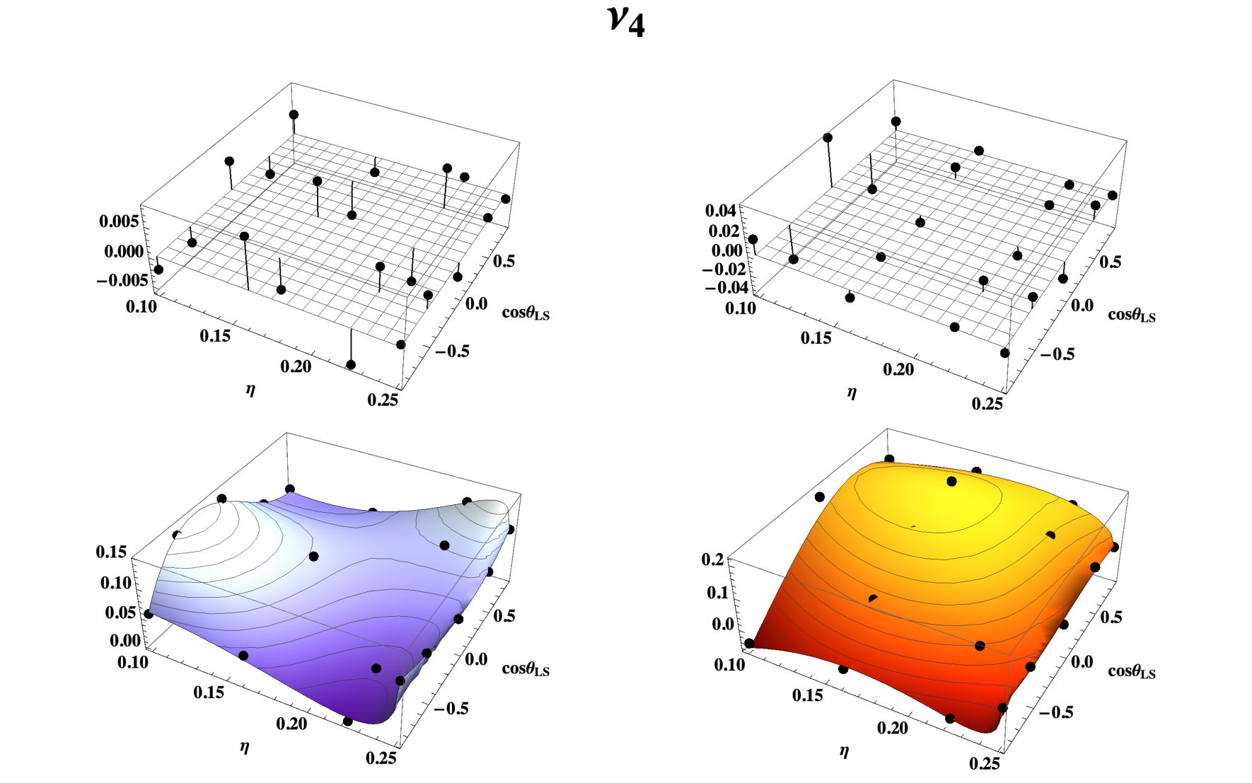 |
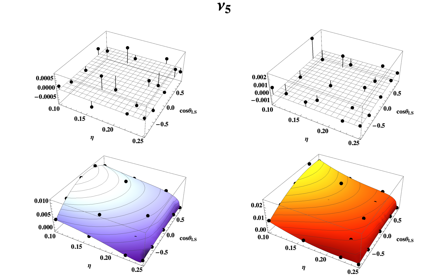 |
 |
 |


References
- Aasi et al. (2015) J. Aasi et al. (LIGO Scientific), Class. Quant. Grav. 32, 074001 (2015), arXiv:1411.4547 [gr-qc] .
- Acernese et al. (2015) F. Acernese et al. (VIRGO), Class. Quant. Grav. 32, 024001 (2015), arXiv:1408.3978 [gr-qc] .
- Abbott et al. (2019) B. Abbott et al. (LIGO Scientific, Virgo), Phys. Rev. X 9, 031040 (2019), arXiv:1811.12907 [astro-ph.HE] .
- Nitz et al. (2020) A. H. Nitz, T. Dent, G. S. Davies, S. Kumar, C. D. Capano, I. hARRY, S. Mozzon, L. Nuttall, A. Lundgren, and M. Tápai, The Astrophysical Journal 891, 123 (2020).
- Zackay et al. (2019) B. Zackay, L. Dai, T. Venumadhav, J. Roulet, and M. Zaldarriaga, (2019), arXiv:1910.09528 [astro-ph.HE] .
- Venumadhav et al. (2020) T. Venumadhav, B. Zackay, J. Roulet, L. Dai, and M. Zaldarriaga, Phys. Rev. D 101, 083030 (2020), arXiv:1904.07214 [astro-ph.HE] .
- Abbott et al. (2020a) R. Abbott et al. (LIGO Scientific, Virgo), (2020a), arXiv:2010.14527 [gr-qc] .
- Husa et al. (2016) S. Husa, S. Khan, M. Hannam, M. Pürrer, F. Ohme, X. Jiménez Forteza, and A. Bohé, Phys. Rev. D 93, 044006 (2016), arXiv:1508.07250 [gr-qc] .
- Khan et al. (2016) S. Khan, S. Husa, M. Hannam, F. Ohme, M. Pürrer, X. Jiménez Forteza, and A. Bohé, Phys. Rev. D 93, 044007 (2016), arXiv:1508.07253 [gr-qc] .
- Hannam et al. (2014) M. Hannam, P. Schmidt, A. Bohé, L. Haegel, S. Husa, F. Ohme, G. Pratten, and M. Pürrer, Phys. Rev. Lett. 113, 151101 (2014), arXiv:1308.3271 [gr-qc] .
- London et al. (2018) L. London, S. Khan, E. Fauchon-Jones, C. García, M. Hannam, S. Husa, X. Jiménez-Forteza, C. Kalaghatgi, F. Ohme, and F. Pannarale, Phys. Rev. Lett. 120, 161102 (2018), arXiv:1708.00404 [gr-qc] .
- Khan et al. (2019) S. Khan, K. Chatziioannou, M. Hannam, and F. Ohme, Phys. Rev. D100, 024059 (2019), arXiv:1809.10113 [gr-qc] .
- Khan et al. (2020) S. Khan, F. Ohme, K. Chatziioannou, and M. Hannam, Phys. Rev. D 101, 024056 (2020), arXiv:1911.06050 [gr-qc] .
- Pratten et al. (2020a) G. Pratten, S. Husa, C. Garcia-Quiros, M. Colleoni, A. Ramos-Buades, H. Estelles, and R. Jaume, (2020a), arXiv:2001.11412 [gr-qc] .
- García-Quirós et al. (2020) C. García-Quirós, M. Colleoni, S. Husa, H. Estellés, G. Pratten, A. Ramos-Buades, M. Mateu-Lucena, and R. Jaume, (2020), arXiv:2001.10914 [gr-qc] .
- Pratten et al. (2020b) G. Pratten et al., (2020b), arXiv:2004.06503 [gr-qc] .
- Thompson et al. (2020) J. E. Thompson, E. Fauchon-Jones, S. Khan, E. Nitoglia, F. Pannarale, T. Dietrich, and M. Hannam, Phys. Rev. D 101, 124059 (2020), arXiv:2002.08383 [gr-qc] .
- Estellés et al. (2020a) H. Estellés, A. Ramos-Buades, S. Husa, C. García-Quirós, M. Colleoni, L. Haegel, and R. Jaume, (2020a), arXiv:2004.08302 [gr-qc] .
- Estellés et al. (2020b) H. Estellés, S. Husa, M. Colleoni, D. Keitel, M. Mateu-Lucena, C. García-Quirós, A. Ramos-Buades, and A. Borchers, (2020b), arXiv:2012.11923 [gr-qc] .
- Taracchini et al. (2012) A. Taracchini, Y. Pan, A. Buonanno, E. Barausse, M. Boyle, T. Chu, G. Lovelace, H. P. Pfeiffer, and M. A. Scheel, Phys. Rev. D 86, 024011 (2012), arXiv:1202.0790 [gr-qc] .
- Pan et al. (2014) Y. Pan, A. Buonanno, A. Taracchini, L. E. Kidder, A. H. Mroué, H. P. Pfeiffer, M. A. Scheel, and B. Szilágyi, Phys. Rev. D89, 084006 (2014), arXiv:1307.6232 [gr-qc] .
- Taracchini et al. (2014) A. Taracchini et al., Phys. Rev. D89, 061502 (2014), arXiv:1311.2544 [gr-qc] .
- Bohé et al. (2017) A. Bohé et al., Phys. Rev. D 95, 044028 (2017), arXiv:1611.03703 [gr-qc] .
- Cotesta et al. (2018) R. Cotesta, A. Buonanno, A. Bohé, A. Taracchini, I. Hinder, and S. Ossokine, Phys. Rev. D 98, 084028 (2018), arXiv:1803.10701 [gr-qc] .
- Ossokine et al. (2020) S. Ossokine et al., Phys. Rev. D 102, 044055 (2020), arXiv:2004.09442 [gr-qc] .
- Matas et al. (2020) A. Matas et al., Phys. Rev. D 102, 043023 (2020), arXiv:2004.10001 [gr-qc] .
- Ramos-Buades et al. (2020) A. Ramos-Buades, P. Schmidt, G. Pratten, and S. Husa, Phys. Rev. D 101, 103014 (2020), arXiv:2001.10936 [gr-qc] .
- Blackman et al. (2017a) J. Blackman, S. E. Field, M. A. Scheel, C. R. Galley, D. A. Hemberger, P. Schmidt, and R. Smith, Phys. Rev. D 95, 104023 (2017a), arXiv:1701.00550 [gr-qc] .
- Varma et al. (2019a) V. Varma, S. E. Field, M. A. Scheel, J. Blackman, L. E. Kidder, and H. P. Pfeiffer, Phys. Rev. D 99, 064045 (2019a), arXiv:1812.07865 [gr-qc] .
- Apostolatos et al. (1994) T. A. Apostolatos, C. Cutler, G. J. Sussman, and K. S. Thorne, Phys. Rev. D 49, 6274 (1994).
- Kidder (1995) L. E. Kidder, Phys. Rev. D 52, 821 (1995), arXiv:gr-qc/9506022 .
- Schmidt et al. (2011) P. Schmidt, M. Hannam, S. Husa, and P. Ajith, Phys. Rev. D84, 024046 (2011), arXiv:1012.2879 [gr-qc] .
- Schmidt et al. (2012) P. Schmidt, M. Hannam, and S. Husa, Phys. Rev. D 86, 104063 (2012), arXiv:1207.3088 [gr-qc] .
- Blackman et al. (2017b) J. Blackman, S. E. Field, M. A. Scheel, C. R. Galley, C. D. Ott, M. Boyle, L. E. Kidder, H. P. Pfeiffer, and B. Szilágyi, Phys. Rev. D 96, 024058 (2017b), arXiv:1705.07089 [gr-qc] .
- Varma et al. (2019b) V. Varma, S. E. Field, M. A. Scheel, J. Blackman, D. Gerosa, L. C. Stein, L. E. Kidder, and H. P. Pfeiffer, Phys. Rev. Research. 1, 033015 (2019b), arXiv:1905.09300 [gr-qc] .
- Ajith et al. (2007) P. Ajith et al., Class. Quant. Grav. 24, S689 (2007), arXiv:0704.3764 [gr-qc] .
- Ajith et al. (2008) P. Ajith et al., Phys. Rev. D 77, 104017 (2008), [Erratum: Phys.Rev.D 79, 129901 (2009)], arXiv:0710.2335 [gr-qc] .
- Ajith et al. (2011) P. Ajith et al., Phys. Rev. Lett. 106, 241101 (2011), arXiv:0909.2867 [gr-qc] .
- Santamaria et al. (2010) L. Santamaria et al., Phys. Rev. D82, 064016 (2010), arXiv:1005.3306 [gr-qc] .
- Pürrer et al. (2016) M. Pürrer, M. Hannam, and F. Ohme, Phys. Rev. D 93, 084042 (2016), arXiv:1512.04955 [gr-qc] .
- Abbott et al. (2020b) B. Abbott et al. (KAGRA, LIGO Scientific, Virgo), Living Rev. Rel. 23, 3 (2020b).
- Fairhurst et al. (2020) S. Fairhurst, R. Green, M. Hannam, and C. Hoy, Phys. Rev. D 102, 041302 (2020), arXiv:1908.00555 [gr-qc] .
- Estellés et al. (2021) H. Estellés, M. Colleoni, C. García-Quirós, S. Husa, D. Keitel, M. Mateu-Lucena, M. d. L. Planas, and A. Ramos-Buades, (2021), arXiv:2105.05872 [gr-qc] .
- Fauchon-Jones et al. (2021) E. Fauchon-Jones, E. Hamilton, C. Kalaghatgi, S. Ghosh, M. Hannam, C. Hoy, S. Khan, P. Kolitsidou, L. London, J. Thompson, A. Vañó-Viñuales, and D. Yeeles, (2021), in preparation.
- Pekowsky et al. (2013) L. Pekowsky, R. O’Shaughnessy, J. Healy, and D. Shoemaker, Phys. Rev. D 88, 024040 (2013), arXiv:1304.3176 [gr-qc] .
- Hofmann et al. (2016) F. Hofmann, E. Barausse, and L. Rezzolla, Astrophys. J. Lett. 825, L19 (2016), arXiv:1605.01938 [gr-qc] .
- O’Shaughnessy et al. (2011) R. O’Shaughnessy, B. Vaishnav, J. Healy, Z. Meeks, and D. Shoemaker, Phys. Rev. D84, 124002 (2011), arXiv:1109.5224 [gr-qc] .
- Boyle et al. (2011) M. Boyle, R. Owen, and H. P. Pfeiffer, Phys. Rev. D84, 124011 (2011), arXiv:1110.2965 [gr-qc] .
- Ochsner and O’Shaughnessy (2012) E. Ochsner and R. O’Shaughnessy, Phys. Rev. D86, 104037 (2012), arXiv:1205.2287 [gr-qc] .
- Boyle et al. (2014) M. Boyle, L. E. Kidder, S. Ossokine, and H. P. Pfeiffer, (2014), arXiv:1409.4431 [gr-qc] .
- Hamilton and Hannam (2018) E. Hamilton and M. Hannam, Phys. Rev. D98, 084018 (2018), arXiv:1807.06331 [gr-qc] .
- Chatziioannou et al. (2017) K. Chatziioannou, A. Klein, N. Cornish, and N. Yunes, Phys. Rev. Lett. 118, 051101 (2017), arXiv:1606.03117 [gr-qc] .
- O’Shaughnessy et al. (2013) R. O’Shaughnessy, L. London, J. Healy, and D. Shoemaker, Phys. Rev. D 87, 044038 (2013), arXiv:1209.3712 [gr-qc] .
- Marsat and Baker (2018) S. Marsat and J. G. Baker, (2018), arXiv:1806.10734 [gr-qc] .
- Bruegmann et al. (2008a) B. Bruegmann, J. A. Gonzalez, M. Hannam, S. Husa, and U. Sperhake, Phys. Rev. D77, 124047 (2008a), arXiv:0707.0135 [gr-qc] .
- Kalaghatgi and Hannam (2020) C. Kalaghatgi and M. Hannam, (2020), arXiv:2008.09957 [gr-qc] .
- LIGO Scientific Collaboration (2018) LIGO Scientific Collaboration, “LIGO Algorithm Library - LALSuite,” free software (GPL) (2018).
- Buonanno et al. (2004) A. Buonanno, Y.-b. Chen, Y. Pan, and M. Vallisneri, Phys. Rev. D 70, 104003 (2004), [Erratum: Phys.Rev.D 74, 029902 (2006)], arXiv:gr-qc/0405090 .
- Schmidt et al. (2015) P. Schmidt, F. Ohme, and M. Hannam, Phys. Rev. D 91, 024043 (2015), arXiv:1408.1810 [gr-qc] .
- Abbott et al. (2020c) R. Abbott et al. (LIGO Scientific, Virgo), Astrophys. J. Lett. 896, L44 (2020c), arXiv:2006.12611 [astro-ph.HE] .
- Bruegmann et al. (2008b) B. Bruegmann, J. A. Gonzalez, M. Hannam, S. Husa, U. Sperhake, and W. Tichy, Phys. Rev. D 77, 024027 (2008b), arXiv:gr-qc/0610128 .
- Boyle et al. (2019) M. Boyle et al., Class. Quant. Grav. 36, 195006 (2019), arXiv:1904.04831 [gr-qc] .
- (63) http://www.black-holes.org.
- Jani et al. (2016) K. Jani, J. Healy, J. A. Clark, L. London, P. Laguna, and D. Shoemaker, Class. Quant. Grav. 33, 204001 (2016), arXiv:1605.03204 [gr-qc] .
- (65) http://www.einstein.gatech.edu/catalog/.
- Campanelli et al. (2006) M. Campanelli, C. Lousto, and Y. Zlochower, Phys. Rev. D 74, 041501 (2006), arXiv:gr-qc/0604012 .
- Cook and York (1990) G. B. Cook and J. York, James W., Phys. Rev. D 41, 1077 (1990).
- Oppenheim et al. (1999) A. V. Oppenheim, R. W. Schafer, and J. R. Buck, Discrete-Time Signal Processing (2nd Ed.) (Prentice-Hall, Inc., USA, 1999).
- Wigner (1959) E. P. Wigner, Group theory and its application to the quantum mechanics of atomic spectra (Academic Press, New York, 1959).
- Bowen and York (1980) J. M. Bowen and J. W. York, Jr., Phys. Rev. D 21, 2047 (1980).
- Ruiz et al. (2008) M. Ruiz, M. Alcubierre, D. Núñez, and R. Takahashi, General Relativity and Gravitation 40, 1705 (2008).
- Campanelli et al. (2007) M. Campanelli, C. O. Lousto, Y. Zlochower, B. Krishnan, and D. Merritt, Phys. Rev. D 75, 064030 (2007), arXiv:gr-qc/0612076 .
- Varma et al. (2020) V. Varma, M. Isi, and S. Biscoveanu, Phys. Rev. Lett. 124, 101104 (2020), arXiv:2002.00296 [gr-qc] .
- Cutler and Flanagan (1994) C. Cutler and E. E. Flanagan, Phys. Rev. D49, 2658 (1994), arXiv:gr-qc/9402014 [gr-qc] .
- Poisson and Will (1995) E. Poisson and C. M. Will, Phys. Rev. D 52, 848 (1995), arXiv:gr-qc/9502040 .
- Ajith (2011) P. Ajith, Phys. Rev. D 84, 084037 (2011), arXiv:1107.1267 [gr-qc] .
- Kumar et al. (2016) P. Kumar, T. Chu, H. Fong, H. P. Pfeiffer, M. Boyle, D. A. Hemberger, L. E. Kidder, M. A. Scheel, and B. Szilagyi, Phys. Rev. D 93, 104050 (2016), arXiv:1601.05396 [gr-qc] .
- Chatziioannou et al. (2017) K. Chatziioannou, A. Klein, N. Yunes, and N. Cornish, Phys. Rev. D95, 104004 (2017), arXiv:1703.03967 [gr-qc] .
- Racine (2008) E. Racine, Phys. Rev. D 78, 044021 (2008), arXiv:0803.1820 [gr-qc] .
- Gerosa et al. (2020) D. Gerosa, M. Mould, D. Gangardt, P. Schmidt, G. Pratten, and L. M. Thomas, (2020), arXiv:2011.11948 [gr-qc] .
- Thomas et al. (2020) L. M. Thomas, P. Schmidt, and G. Pratten, (2020), arXiv:2012.02209 [gr-qc] .
- Arun et al. (2009) K. G. Arun, A. Buonanno, G. Faye, and E. Ochsner, Phys. Rev. D79, 104023 (2009), [Erratum: Phys. Rev.D84,049901(2011)], arXiv:0810.5336 [gr-qc] .
- London and Fauchon-Jones (2019) L. London and E. Fauchon-Jones, Class. Quant. Grav. 36, 235015 (2019), arXiv:1810.03550 [gr-qc] .
- London et al. (2020) L. London, E. Fauchon, and EZHamilton, “llondon6/positive: map,” (2020).
- Kesden et al. (2015) M. Kesden, D. Gerosa, R. O’Shaughnessy, E. Berti, and U. Sperhake, Phys. Rev. Lett. 114, 081103 (2015), arXiv:1411.0674 [gr-qc] .
- Klein et al. (2013) A. Klein, N. Cornish, and N. Yunes, Phys. Rev. D 88, 124015 (2013), arXiv:1305.1932 [gr-qc] .
- Chatziioannou et al. (2013) K. Chatziioannou, A. Klein, N. Yunes, and N. Cornish, Phys. Rev. D 88, 063011 (2013), arXiv:1307.4418 [gr-qc] .
- Virtanen et al. (2020) P. Virtanen, R. Gommers, T. E. Oliphant, M. Haberland, T. Reddy, D. Cournapeau, E. Burovski, P. Peterson, W. Weckesser, J. Bright, S. J. van der Walt, M. Brett, J. Wilson, K. J. Millman, N. Mayorov, A. R. J. Nelson, E. Jones, R. Kern, E. Larson, C. J. Carey, İ. Polat, Y. Feng, E. W. Moore, J. VanderPlas, D. Laxalde, J. Perktold, R. Cimrman, I. Henriksen, E. A. Quintero, C. R. Harris, A. M. Archibald, A. H. Ribeiro, F. Pedregosa, P. van Mulbregt, and SciPy 1.0 Contributors, Nature Methods 17, 261 (2020).
- Leaver (1985) E. Leaver, Proc. Roy. Soc. Lond. A A402, 285 (1985).
- Kamaretsos et al. (2012a) I. Kamaretsos, M. Hannam, and B. Sathyaprakash, Phys. Rev. Lett. 109, 141102 (2012a), arXiv:1207.0399 [gr-qc] .
- Kamaretsos et al. (2012b) I. Kamaretsos, M. Hannam, S. Husa, and B. S. Sathyaprakash, Phys. Rev. D 85, 024018 (2012b), arXiv:1107.0854 [gr-qc] .
- Giesler et al. (2019) M. Giesler, M. Isi, M. A. Scheel, and S. Teukolsky, Phys. Rev. X 9, 041060 (2019), arXiv:1903.08284 [gr-qc] .
- (93) LSC, “LIGO Document T1800044-v5,” https://dcc.ligo.org/LIGO-T1800044/public.
- Harry et al. (2016) I. Harry, S. Privitera, A. Bohé, and A. Buonanno, Phys. Rev. D 94, 024012 (2016), arXiv:1603.02444 [gr-qc] .
- Mroue et al. (2013) A. H. Mroue et al., Phys. Rev. Lett. 111, 241104 (2013), arXiv:1304.6077 [gr-qc] .
- Schmidt et al. (2017) P. Schmidt, I. W. Harry, and H. P. Pfeiffer, (2017), arXiv:1703.01076 [gr-qc] .
- Hunter (2007) J. D. Hunter, Computing in Science & Engineering 9, 90 (2007).
- Harris et al. (2020) C. R. Harris, K. J. Millman, S. J. van der Walt, R. Gommers, P. Virtanen, D. Cournapeau, E. Wieser, J. Taylor, S. Berg, N. J. Smith, R. Kern, M. Picus, S. Hoyer, M. H. van Kerkwijk, M. Brett, A. Haldane, J. F. del Río, M. Wiebe, P. Peterson, P. Gérard-Marchant, K. Sheppard, T. Reddy, W. Weckesser, H. Abbasi, C. Gohlke, and T. E. Oliphant, Nature 585, 357 (2020).
- Nitz et al. (2021) A. Nitz, I. Harry, D. Brown, C. M. Biwer, J. Willis, T. D. Canton, C. Capano, T. Dent, L. Pekowsky, A. R. Williamson, G. S. C. Davies, S. De, M. Cabero, B. Machenschalk, P. Kumar, D. Macleod, S. Reyes, dfinstad, F. Pannarale, T. Massinger, S. Kumar, M. Tápai, L. Singer, S. Khan, S. Fairhurst, A. Nielsen, S. Singh, shasvath, B. U. V. Gadre, and I. Dorrington, “gwastro/pycbc: Pycbc release 1.18.1,” (2021).
- Newman and Penrose (1966) E. T. Newman and R. Penrose, Journal of Mathematical Physics 7, 863 (1966), https://doi.org/10.1063/1.1931221 .
- Shah and Whiting (2016) A. G. Shah and B. F. Whiting, Gen. Rel. Grav. 48, 78 (2016), arXiv:1503.02618 [gr-qc] .