Triad second renormalization groupPreprint: KANAZAWA-21-03

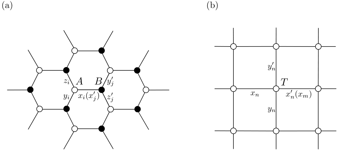
We begin with considering a homogeneous tensor network on a honeycomb lattice:

where $b$ and $w$ are the sets of black and white lattice points, and $\mathrm{Tr}$ is the summation over all tensor indices $x,y,z=1,2,\cdots,\chi$. The link $x_{i}$ is identified to $x^{\prime}_{j}$ where $j$ is the nearest neighbor site of $i$ in the $x$ direction, and the same applies to $y^{\prime}$ and $z^{\prime}$. Fig. 1 (a) shows the tensor network on the honeycomb lattice. We assume that $A$ and $B$ are totally symmetric tensors for simplicity of explanation. It is straightforward to extend the algorithm presented in this section to the non-symmetric case.

The singular value decomposition (SVD) of an $n\times n$ matrix $M$, which is used for the coarse graining, is defined in the standard manner as

where $\Lambda$ is an $n\times n$ diagonal matrix in which singular values are sorted in the descending order, and $U$ and $V$ are $n\times n$ unitary matrices. Taking the $k$ largest singular values ($k<n$) gives the best $k$-rank approximation of $M$ as

where $C_{Im}=(U\sqrt{\Lambda})_{Im}$ and $D_{Jm}=(\sqrt{\Lambda}V^{\dagger})_{mJ}$.

The partition function is evaluated by the TRG using the SVD such that the form of Eq. (1) is kept at $n$th renormalization step with $A^{(n)}$ and $B^{(n)}$. Consider a $\chi^{2}\times\chi^{2}$ matrix $M^{(n)}$ defined by ¹¹ 1 The comma in $M_{ij,kl}$ is employed to regard a tensor $M_{ijkl}$ as a matrix with the column $i,j$ and the row $k,l$. Unless otherwise noted, $\sum_{i}$ denotes $\sum_{i=1}^{\chi}$ in this paper.

With the Eqs. (2) and (3), we have a $\chi$-rank approximation of $M^{(n)}$ as

Fig. 2 shows the transformation of $M^{(n)}$ from Eq. (4) to (5). As shown in Fig. 3, we arrive at Eq. (1) again with renormalized tensors,

In case of finite volume lattice of $V=2\times 3^{N}$ with the center symmetric boundary condition, the renormalization is completed in $N$ steps. Finally we can evaluate $Z$ from two tensors $A^{(N)}$ and $B^{(N)}$ as $Z\approx\sum_{x,y,z}A^{(N)}_{xyz}B^{(N)}_{xyz}$ where $A^{(0)}$ and $B^{(0)}$ are the initial tensors.

Although the SVD gives the best approximation of tensors locally, it does not always give the best one for $Z$ because the rest of tenor network (i.e. the environment for $M$) is ignored. The second renormalization group (SRG) method incorporates the influence of environments into the decomposition of $M$ so that $Z$ is well approximated.

In order to formulate the SRG, let us express $Z$ as

where $M$ is given as Eq. (4) from $A$ and $B$. As shown in Fig. 4, $M^{\rm e}$ is the rest tensor network excluding $M$ from $Z$. It is difficult to evaluate $M^{\rm e}$ exactly for a large volume lattice because $M^{\rm e}$ contains many tensor contractions.

One may evaluate $M^{\rm e}$ iteratively using the TRG method as shown in Fig. 5 where $E^{(0)}=M^{{\rm e}}$ at the first renormalization step. The coarse-grained environments approximately satisfy a recurrence relation,

We rather define the $i$-th scale environment tensor $E^{(i)}$ with Eq. (8) by solving it $N-1$ times from $E^{(N)}_{ab,cd}=\delta_{ac}\delta_{bd}$ (backward step) and finally obtain $E^{(0)}$ which is an approximate estimate of $M^{\rm e}$. Before starting the backward step, we perform the usual TRG procedure (the forward step) to generate $C^{(n)}$ and $D^{(n)}$ ($n=1,2,...,N-1$). See Fig. 6 for a schematic representation of the recurrence relation of Eq. (8). In the figure we have to take care that the bold circle with internal four links are not four rank-3 tensors but a rank-$4$ environment tensor $E^{(n+1)}$. We should also note that $E^{(n+1)}$ has coarse grained indices which emerge when dropping Fig. 5 (e).

Once $M^{\rm e}$ is obtained, $M$ is decomposed by the fundamental procedure of SRG as follows. We firstly decompose $M^{\rm e}$ by the SVD as $M^{\rm e}=U_{\rm e}\Lambda_{\rm e}V_{\rm e}^{\dagger}$ and define

Then we also decompose $\tilde{M}$ by the SVD as

Since $Z={\rm Tr}\,\tilde{M}$, the (truncated) SVD of $\tilde{M}$ gives the best approximation of $Z$. From Eq. (9) and Eq. (10), we have an approximation of $M$ as

where $C_{Im}=(V_{\rm e}\sqrt{\Lambda_{\rm e}}^{-1}\tilde{U}\sqrt{\tilde{\Lambda}})_{Im}$ and $D_{Jm}=(\sqrt{\tilde{\Lambda}}\tilde{V}^{\dagger}\sqrt{\Lambda_{\rm e}}^{-1}U_{\rm e}^{\dagger})_{mJ}$. Applying these procedures in Eq. (9)–(11) to $M^{(n)}$ given by Eq. (4), the truncation error of the whole tensor network is minimized, rather than that of $M^{(n)}$.

In this way, the SRG for the honeycomb lattice Xie:2009zzd can capture the environment effects and reduce the truncation error in the coarse-graining steps. The computational costs of TRG and SRG scale with $\chi^{6}$ since the SVD and the recurrence relation have a scaling of $\chi^{6}$ where the cost of SVD is reduced to $\chi^{5}$ by using the randomized SVD, and the cost of TRG can be reduced in this sense. Numerical results presented in Fig. 4 of Ref. Xie:2009zzd show that the error of TRG is drastically reduced by the SRG.

We consider a homogeneous tensor network of rank-4 tensors $T_{ijkl}$ ($i,j,k,l=1,\ldots,\chi$) on the two dimensional square lattice :

where $\Gamma$ is the set of all lattice sites. As can be seen in Fig. 1 (b), $x^{\prime}_{n}$ coincides with the index $x_{m}$ of the tensor on the nearest neighbor site $m$ in the positive $x$ direction, and the same applies to $y^{\prime}_{n}$. Therefore each summation is the contraction over the shared indices.

The renormalization of HOTRG is carried out for $x$ and $y$ directions alternately. We first consider the renormalization along the $y$ axis. Let $M^{(n)}$ be rank-6 tensor made of two tensors $T^{(n)}$ as

where $x=x_{1}\otimes x_{2}$ and $x^{\prime}=x_{1}^{\prime}\otimes x_{2}^{\prime}$, which is shown in Fig. 7 (a).

Let us consider a matrix representation of $M$ as $M^{\prime}_{x,x^{\prime}yy^{\prime}}\equiv M_{xx^{\prime}yy^{\prime}}^{(n)}$ to create an isometry $U$ by which the tensor network is renormalized. We diagonalize $K\equiv M^{\prime}M^{\prime{\dagger}}$ as

where ${\Lambda}$ is a diagonal matrix in which eigenvalues $\lambda_{i}$ are sorted in the descending order, and $U$ is the unitary matrix. We employ $U$ as the isometry ²² 2 We actually choose the isometry $U$ from two unitary matrices: the left unitary matrix $U_{L}$ defined by Eq. (14) and the right unitary matrix $U_{R}$ defined by diagonalizing $\tilde{K}=M^{\prime}{M^{\prime}}^{\dagger}$ for $M^{\prime}_{x^{\prime},xyy^{\prime}}\equiv M_{xx^{\prime}yy^{\prime}}$ as $\tilde{K}=U_{R}\Lambda_{R}{U_{R}}^{\dagger}$. Then $U$ is chosen to be $U=U_{L}$ for $\epsilon_{L}\leq\epsilon_{R}$ and $U=U_{R}^{\ast}$ for $\epsilon_{R}<\epsilon_{L}$ where $\epsilon_{Q}\equiv\sum_{i>\chi}\lambda_{Q,i}$ for $Q=L,R$. See Ref. HOTRG for the detail. and define a renormalized tensor $T^{(n+1)}$ as

Note that $x,y$ are truncated indices which run from $1$ to $\chi$ although $i,j$ run from $1$ to $\chi^{2}$. Fig. 7 (b) shows the renormalization of the 2d HOTRG.

Thus $Z$ is again expressed as Eq. (12) with Eq. (15). After finishing the renormalization along the $y$ direction, we move on to the renormalization along the $x$ direction. This can be carried out by simply repeating Eqs. (13)–(15) because the ordering of indices in the lhs of Eq. (15) have already changed to be able to do that. The HOTRG ends in $N$ steps for a finite volume lattice of $V=2^{N}(=2^{\frac{N}{2}}\times 2^{\frac{N}{2}})$ where $N$ is an even integer. We finally obtain the value of $Z$ by evaluating $Z\approx\sum_{x,y}T^{(N)}_{xxyy}$ where $T^{(0)}$ is an initial tensor.

Since the isometry $U$ is determined from the local diagonalization for $K$ in Eq. (14), the HOTRG also ignores the influence of environment tensors as in case of TRG. In Ref. HOTRG, the second renormalization group for the HOTRG is proposed as the HOSRG. In the HOSRG, the HOTRG is used only for obtaining the initial set of $T^{(n)}$ and $U^{(n)}$ for $n=0,1,\ldots,N-1$. Then $T^{(n)}$ and $U^{(n)}$ are updated by using the recurrence relation for the environment tensors and a diagonalization of the bond density matrix. In this paper, we employ $X^{(n)}$ as described in Ref. MERAupdate and defined below to update $U^{(n)}$ instead of using the bond density matrix because the computational cost is reduced.

Let us express $Z$ as

where $T^{\rm e}$ is the environments of $T$, which is defined by removing $T$ from $Z$ as shown in Fig. 8. As in case of SRG, we evaluate $T^{\rm e}$ iteratively using the HOTRG method as shown in Fig. 9. For $E^{(0)}=T^{{\rm e}}$ which is the environment for $T^{(0)}$, the $n$-scale environment $E^{(n)}$ contains $2^{N}-2^{n}$ tensors of the scale $n$. The environment tensors approximately satisfy a recurrence relation,

and we define the $i$-scale $E^{(i)}$ with the recurrence relation by solving it from $E^{(N)}_{ab,cd}=\delta_{ab}\delta_{cd}$. Fig. 10 shows a schematic representation of the recurrence relation Eq. (17).

Once the environment is obtained, the isometry $U^{(n)}$ is updated from $X^{(n)}$ defined by

Fig. 11 shows $X^{(n)}$. We decompose $X^{(n)}$ by the SVD as

Then $U^{(n)}$ is updated by

We should note here that $Z={\rm Tr}(U^{(n){\dagger}}X^{(n)})={U^{(n)}}^{\dagger}_{a,id}X^{(n)}_{id,a}\approx\sum_{m}\sigma_{m}$ and $U^{(n)}$ is updated in a sense that $Z$ is well approximated.

The HOSRG is given in 2d square lattice of $V=2^{N}$ (with the periodic boundary condition) as follows: we compute all of the $T^{(n)}$ and $U^{(n)}$ ($n=0,1,\ldots,N-1$) by the HOTRG. Then, for these initial sets of $T^{(n)}$ and $U^{(n)}$, we employ a forward-backward algorithm that repeats (i) and (ii) $m$ times (sweeps) where $m$ is chosen so that converged or better results are obtained ³³ 3 $m=5\sim 10$ is large enough in the actual computations of 2d Ising model on $V=2^{50}$ presented in section IV. :

• (i)

  $E^{(n)}$ ($n=1,2,\ldots,N$) are computed by solving the recurrence relation Eq. (17).

• (ii)

  Two procedures are repeated for $n=0,1,\ldots,N-1$: $U^{(n)}$ is updated by Eqs. (18)–(20) from $E^{(n+1)},T^{(n)},U^{(n)}$. Then $T^{(n+1)}$ is updated by Eq. (15) from $T^{(n)}$ and the new $U^{(n)}$.

Finally we evaluate $Z\approx\sum_{x,y}T^{(N)}_{xxyy}$ in the HOSRG as well as the HOTRG.

The computational costs of HOTRG/HOSRG scale with ${\cal O}(N\chi^{7})$ and ${\cal O}(mN\chi^{7})$, respectively, since the contraction in Eq. (15) takes a cost of $N\chi^{7}$ and the recurrence relation and $X^{(n)}$ in Eq. (18) are evaluated in a cost of $mN\chi^{7}$. Fig. 4 of Ref. HOTRG, Fig. 10 of Ref. HOTRG_pbc and Figs. 21–23 presented in section IV show that the HOSRG significantly improves the accuracy of results.

We consider a lattice model with local interactions on $d$ dimensional hyper cubic lattice. The partition function of a translational invariant theory is given by a homogeneous tensor network of a rank-$2d$ tensor $T$. Then $T$ is naturally obtained as a polyadic decomposition:

since $2d$ hopping terms stemmed from a site provide $2d$ $W_{rj}$ factors.

A triad representation of $T$ is hidden in Eq. (21). For instance, in 3 dimensions, we have

where

Note that this kind of representation is not unique because we can interchange $W^{(i)}\leftrightarrow W^{(j)}$ for $A,B,C,D$. In Ref. Kadoh:2019kqk, the computational cost is reduced by applying the HOTRG-like renormalization to the triad tensor network because all of the tensors are made of rank-$3$ tensors in the triad tensor network.

Let us consider two dimensional case of the triad representation like Eq. (22) as

where

The tensor network of Eq. (27) is introduced by setting $T$ of Eq. (12) to Eq. (27). Fig. 12 shows the triad representation and its tensor network, respectively. In two dimensions, the triad network with the periodic boundary condition can be regarded as one on a honeycomb lattice with unusual boundary condition. ⁴⁴ 4 In Ref. Zhao2010, the tensor network on a square lattice is embedded into one on a honeycomb lattice with an enlarged intermediate index that runs from $1$ to $\chi^{2}$.

The triad TRG in two dimensions is simply introduced by setting the rank-$4$ tensor $T$ to Eq. (27) in the HOTRG algorithm. The renormalized tensor given by Eq. (15) can be decomposed into renormalized triads by the SVD as

Thus the tensor renormalization is realized on the triad network. The cost of contracting indices in Eq. (15) is reduced to ${\cal O}(\chi^{6})$ using Eq. (27) for $M^{(n)}$. Note that other parts such as creating the isometry $U^{(n)}$ shown in Eq. (14) and the SVD of Eq. (29) scales with $\chi^{6}$ without Eq. (27). With the help of the randomized SVD (RSVD), the cost is further reduced to $\chi^{5}$. Thus the cost of triad TRG method in two dimensions scales with ${\cal O}(N\chi^{6})$ (or ${\cal O}(N\chi^{5})$ with the RSVD).

We introduce a preliminary SRG algorithm on a triad network before the triad SRG is defined in the next section. This algorithm is simply given by setting $T$ in the HOSRG to Eq. (27). The cost of the HOSRG is then reduced to ${\cal O}(\chi^{6})$ as seen below.

The leading cost of the HOSRG, which is $\chi^{7}$, comes from three parts of its algorithm: the HOTRG in the first round, the evaluation of the environment tensors solving the recurrence relation in Eq. (17) and update of isometry from $X^{(n)}$ in Eq. (18). Instead of the HOTRG, we use the triad TRG to give the initial set of tensors $A^{(n)},B^{(n)}$ and isometries $U^{(n)}$, and the cost of this part is reduced to $\chi^{6}$.

The recurrence relation with Eq. (27) is given by

where $E^{(N)}_{ab,cd}=\delta_{ab}\delta_{cd}$. Fig. 13 (a) shows the recurrence relation of Eq. (30). Contracting links in the order of $(d,e)\rightarrow(a,c)\rightarrow(b,g)$ leads to Fig. 13 (b), and these contractions take at most a cost of $\chi^{6}$. Thus we find that the cost of solving the recurrence relation scales with $\chi^{6}$.

Fig. 14 shows $X^{(n)}$ in which $T$ is replaced by Eq. (27) as

Fig. 14 (b) is obtained from Fig. 14 (a) by contracting links in the order of $(g,i^{\prime})\rightarrow(j,j^{\prime},b)\rightarrow(c,e,f)$. Thus we can evaluate $X^{(n)}$ within the cost of $\chi^{6}$. Once $X^{(n)}$ is obtained, $U^{(n)}$ is updated by Eqs. (19) and (20) in the cost of $\chi^{4}$.

The renormalized rank-$4$ tensor $T^{(n+1)}$ is given by the updated $U^{(n)}$ according to Eq. (15). Once $T^{(n+1)}$ and its environment $E^{(n+1)}$ are given, renormalized triads $A^{(n+1)}$ and $B^{(n+1)}$ are obtained from the fundamental procedure of SRG presented in Eqs. (9)–(11). Setting $T^{(n+1)},E^{(n+1)}$ to $M,M^{\rm e}$, respectively, we find a triad representation of the next step:

where the definitions of $A$ and $B$ can be read from $C$ and $D$ of Eq. (11). This procedure scales with $\chi^{6}$ as it consists of the matrix products and the SVDs for $\chi^{2}\times\chi^{2}$ matrices.

The preliminary algorithm in 2d square lattice of $V=2^{N}$ with PBC is summarized below. The initial set of $A^{(n)},B^{(n)}$ and $U^{(n)}$ ($n=0,1,\ldots,N-1$) are generated by the triad TRG. We then repeat (i) and (ii) $m$ times (sweeps):

• (i)

  $E^{(n)}$ ($n=1,2,\ldots,N$) are computed by solving the recurrence relation Eq. (30).

• (ii)

  Two procedures are repeated for $n=0,1,\ldots,N-1$: $U^{(n)}$ is updated by using $X^{(n)}$ in Eq. (31) and its SVD shown as Eqs. (19) and (20) from $E^{(n+1)},A^{(n)},B^{(n)},U^{(n)}$. Then $A^{(n+1)},B^{(n+1)}$ are updated by Eqs. (15) and (32) from $E^{(n+1)},A^{(n)},B^{(n)}$ and the new $U^{(n)}$.

where $m$ is chosen so that converged or better results are obtained. We finally evaluate $Z\approx\sum_{i,j,a}A^{(N)}_{ija}B^{(N)}_{aji}$, or $Z\approx\sum_{i,j}T^{(N)}_{iijj}$ with $T^{(N)}$ in the last step (ii). The cost of this algorithm scales with ${\cal O}(mN\chi^{6})$.

The preliminary algorithm shown in the previous section was obtained by setting $T$ to the triad representation Eq. (27) in the HOSRG. We define the triad SRG further decomposing environment and intermediate tensors with the randomized SVD(RSVD) (See, for example, Refs.RSVD; RSVDTRG for the details of RSVD). The algorithm proposed here scales with $\chi^{5}$.

The $\chi^{6}$ dependence on the cost of the preliminary algorithm is originated from four parts: (i) the triad TRG in the first round, (ii) the creation of the environment tensors with the recurrence relation Eq. (30), (iii) the update of isometry with $X^{(n)}$ given by Eq. (31), (iv) the reconstruction of the triads shown in Eq. (32). With the RSVD, the cost of (i) is reduced to $\chi^{5}$ as described in Ref. Kadoh:2019kqk. Decomposing the environment tensor reduces the cost of (ii) to $\chi^{5}$. The cost of (iii) is also reduced to $\chi^{5}$ by decomposing an intermediate tensor ${\cal M}$ defined later. For (iv), with the decomposed ${\cal M}$, the renormalized triads are obtained at a cost of $\chi^{5}$. We see these points in detail below.

In the triad TRG, the leading cost comes from creating the isometry $U^{(n)}$ and the renormalized triads $A^{(n+1)}$ and $B^{(n+1)}$ (See Eqs. (13), (14), (15) with Eqs. (27) and (32)). Fig. 15 (a) shows $K=M^{\dagger}M$ with the triads. A two-loop graph with external four legs shown in Fig. 15 (b) is obtained in a cost of $\chi^{5}$ by contracting indices $a,a^{\prime},x_{1}^{\prime},x_{2}^{\prime},y,y^{\prime}$ from (a). We can diagonalize the two-loop graph to create the isometry $U^{(n)}$ within $\chi^{5}$ by using the randomized tricks such as the RSVD twice. See the appendix Ref. Kadoh:2019kqk for more details. Using $U^{(n)}$, the renormalized triads are obtained as in Fig. 16. We again encounter a two loop graph shown in Fig. 16 (b) by contracting indices $i^{\prime},j,d$ where

The single use of RSVD again reduces the cost of decomposing Fig. 16 (b) into Fig. 16 (c). Thus the cost of triad TRG becomes $\chi^{5}$.

The rank-$4$ environment tensor $E^{(n)}$ is solved iteratively by using the recurrence relation Eq. (30). With the RSVD, $E^{(n)}$ is obtained as a product of two rank-$3$ tensors $E_{1}^{(n)}$ and $E_{2}^{(n)}$:

The cost of computing the environment tensors is then reduced to $\chi^{5}$ by employing Eq. (36) in its rhs. Fig. 17 shows how to obtain a triad form of the environment in Eq. (36) using Eq. (30). Thank to Eq. (36), a two loop graph shown in Fig. 17 (b) is obtained by contracting indices $a,c,e$ of Fig. 17 (a). ⁵⁵ 5 For $n=N$, a single loop graph actually appears. Fig. 17 (c) is also obtained at the same cost in that case. For such a multi loop graph, the RSVD is employed to obtain Fig. 17 (c) in a cost of $\chi^{5}$. We can obtain $E^{(n)}$ of rank-$4$ as its rank-$3$ representation Eq. (36) within a cost of $\chi^{5}$.

To create the isometry in lower cost, we decompose ${\cal M}^{(n)}$ given by Eq. (34) using the SRG procedure. ⁶⁶ 6 One may locally decompose ${\cal M}$, but in that case we found that accuracy of the free energy becomes worse. The partition function may be expressed as

Since $Z\approx{\rm Tr}(T^{(n)}T^{{\rm e}(n)})$ at $n$th renormalization step with $E^{(n)}=T^{{\rm e}(n)}$, we may define ${\cal M}^{{\rm e}\,(n)}$ as

Figs. 18 and 19 show ${\cal M}^{{\rm e}\,(n)}$ and a clear relationship between $(T^{(n+1)},T^{{\rm e}(n+1)})$ and $({\cal M}^{(n)},{\cal M}^{{\rm e}\,(n)})$.

We employ the SRG procedure given in Eqs. (9)–(11) with the RSVD to decompose ${\cal M}$. ${\cal M}^{(n)}$ and ${\cal M}^{{\rm e}\,(n)}$ are set to $M$ and $M^{\rm e}$, respectively. We decompose $M^{\rm e}$ as $M^{\rm e}\approx U_{\rm e}\Lambda^{\prime}_{\rm e}V_{\rm e}^{\dagger}$ in a similar way to the RSVD but with a thick QR decomposition and a thick SVD with a cost of $\chi^{5}$. The decomposition procedure is applied directly to the matrix product form of ${\cal M}^{{\rm e}\,(n)}$ shown in Fig. 18. Then $U_{\rm e}$ and $V_{\rm e}$ are obtained as $\chi^{2}\times\chi^{2}$ unitary matrices, while $\Lambda^{\prime}_{\rm e}$ is a $p\chi\times p\chi$ diagonal matrix in which singular values $\sigma_{i}$ are sorted in the descending order. ⁷⁷ 7 $p$ is a tunable parameter, which is taken to be O(1) so that the leading cost is kept. In our implementation, $p$ is set to be 2. We enlarge $\Lambda^{\prime}_{\rm e}$ to a $\chi^{2}\times\chi^{2}$ diagonal matrix $\Lambda_{\rm e}$ by supplementing $\epsilon$ in its diagonal elements as ⁸⁸ 8 We need the $\chi^{2}\times\chi^{2}$ matrix $\Lambda_{\rm e}^{-1}$, not $\chi\times\chi$ one, to read $M$ from $\tilde{M}$.

where $\epsilon=\sigma_{1}\times 10^{-15}$. Thus we have $M^{\rm e}\approx U_{\rm e}\Lambda_{\rm e}V_{\rm e}^{\dagger}$ where $U_{\rm e},V_{\rm e},\Lambda_{\rm e}$ are $\chi^{2}\times\chi^{2}$ matrices. The RSVD is again applied directly to a matrix product $\tilde{M}$ defined by Eq. (9), and we obtain $\tilde{M}\approx\tilde{U}\tilde{\Lambda}\tilde{V}^{\dagger}$ in a cost of $\chi^{5}$. Thus we have the global decomposition of $\mathcal{M}$ in Eq. (11) as

where $C^{(n)}_{ij,m}=(V_{\rm e}\sqrt{\Lambda_{\rm e}}^{-1}\tilde{U}\sqrt{\tilde{\Lambda}})_{ij,m}$ and $D^{(n)}_{ij,m}=(\sqrt{\tilde{\Lambda}}\tilde{V}^{\dagger}\sqrt{\Lambda_{\rm e}}^{-1}U_{\rm e}^{\dagger})_{m,ij}$, which are computed within $\chi^{5}$.

$X^{(n)}$ is defined with the decomposed ${\cal M}$ as

Note that Eq. (42) and Eq. (31) are the same but $A$ and $B$ of Eq. (31), which correspond to $\mathcal{M}$, are replaced by Eq. (41). Fig. 20 shows a graphical representation of $X^{(n)}$ given by Eq. (42). Fig. 20 (b) is obtained in a cost of $\chi^{5}$ from Fig. 20 (a) by contracting indices in the order of $(f,e,i^{\prime})\rightarrow(b,j^{\prime},g)\rightarrow(c,\delta)$. Once $X^{(n)}$ is obtained, the isometry $U^{(n)}$ is updated by Eqs. (19) and (20).

With the updated isometry $U^{(n)}$ and the decomposed ${\cal M}^{(n)}$, the renormalized triads are simply defined by

where $C^{(n)},D^{(n)}$ are given by Eq. (41), and ${\cal U}^{(n)},{\cal D}^{(n)}$ are given by Eqs. (33) and (35) in which $U^{(n)}$ is updated by Eq. (19), (20) and (42).

The triad SRG is thus given in 2d square lattice of $V=2^{N}$ with PBC as follows. We first generate the initial set of $A^{(n)},B^{(n)}$ and $U^{(n)}$ ($n=0,1,\ldots,N-1$) by the triad TRG with the $\chi^{5}$ algorithm reviewed above in this subsection. We then repeat (i) and (ii) $m$ times (sweeps):

• (i)

  $E^{(n)}$ ($n=1,2,\ldots,N$) are computed by solving Eq. (30) iteratively with Eq. (36).

• (ii)

  Three procedures are repeated for $n=0,1,\ldots,N-1$: ${\cal M}^{(n)}$ is decomposed as Eq. (41) using Eqs. (33), (34), (35) and (38) from $A^{(n)},B^{(n)},E^{(n+1)}$ and $U^{(n)}$. Then $U^{(n)}$ is updated by Eq. (42) and its SVD shown as Eqs. (19) and (20) from $E^{(n+1)},A^{(n)},B^{(n)},U^{(n)}$. Then $A^{(n+1)},B^{(n+1)}$ are updated by Eqs. (43) and (44) from $E^{(n+1)},A^{(n)},B^{(n)}$ and the new $U^{(n)}$.

where $m$ is chosen so that converged or better results are obtained. We finally evaluate $Z\approx\sum_{i,j,a}A^{(N)}_{ija}B^{(N)}_{aji}$. The cost of this algorithm scales with ${\cal O}(mN\chi^{5})$.