Integrability and Conformal Bootstrap: One Dimensional Defect CFTPreprint: APS/123-QED
Abstract
In this letter we study how the exact non-perturbative integrability methods in Super–Yang-Mills can work efficiently together with the numerical conformal bootstrap techniques to go beyond the spectral observables and access previously unreachable quantities such as correlation functions at finite coupling. In the setup of 1D defect CFT living on a Maldacena-Wilson line, we managed to compute with good precision a non-supersymmetric structure constant for a wide range of the ‘t Hooft coupling. Our result is particularly precise at strong coupling and matches well with the recent analytic results of Meneghelli and Ferrero.
I Introduction
When it comes to non-perturbative calculations in QFTs, the number of tools is rather limited. Monte Carlo simulation could give rather accurate results in some theories. In a smaller set of integrable QFTs one can get access to a large number of observables, but usually those theories are limited to 2D. There are a few exceptions, such as =4 supersymmetric Yang-Mills (SYM) in 4D, where integrability gives access to non-perturbative physics. The most accurate non-perturbative results are limited to the spectrum of anomalous dimensions, where the Quantum Spectral Curve (QSC) Gromov et al. 2014; Gromov et al. 2015a method allows one to get extremely precise results at ‘t Hooft coupling (for example digits in Gromov et al. 2015b for the BFKL Pomeron intercept).
In this paper we focus on planar =4 SYM. As a conformal theory, for its complete solution, in addition to the dimensions of the operators, one also needs to know the OPE coefficients or structure constants. Even though there have been many exciting applications of integrability to the study of the structure constants Basso et al. 2015; Cavaglià et al. 2018; Jiang et al. 2019; Cavaglià et al. 2021, these results are either limited to perturbation theory, infinitely long operators, strongly -deformed (Fishnet) theories, or are not explicit enough for numerical evaluation.
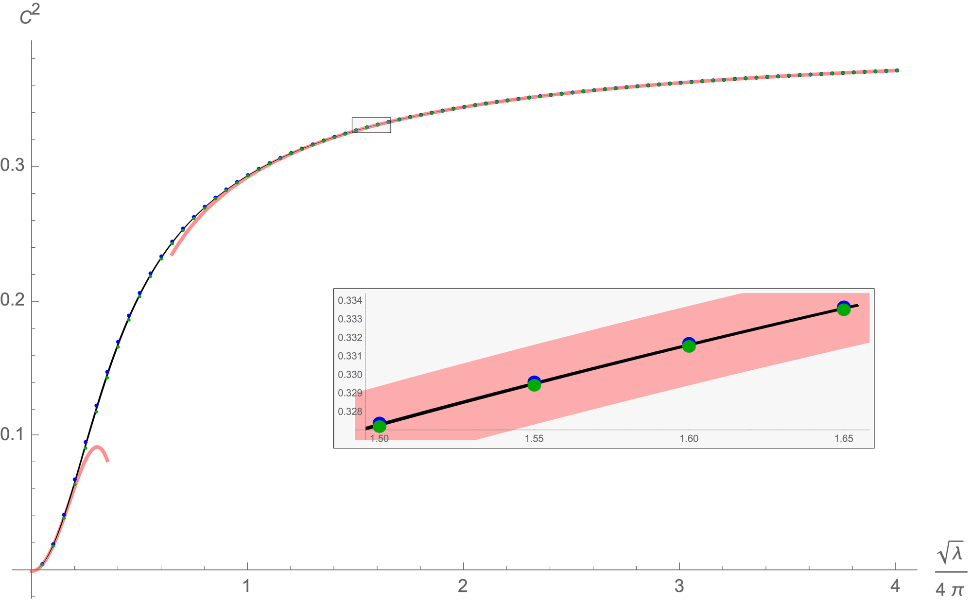
Another powerful non-perturbative method to study CFTs is the Numerical Conformal Bootstrap (NCB) (see Simmons-Duffin 2016; Poland et al. 2019; Chester 2019 for some reviews). It allows one to identify prohibited domains for the conformal dimensions or OPE coefficients given the symmetries of the CFT as an input.
In this paper we join together the two powerful methods of QSC and NCB to obtain accurate values for a nontrivial structure constant in a wide range of the coupling (see Fig. 1).
Even though there is hope for an integrability based non-perturbative analytical solution of the theory, for example built upon the SoV approach Cavaglià et al. 2018; Giombi and Komatsu 2018, it is crucial to have an alternative numerical method which would generate high precision data for future comparison.
II Setup
Here we focus on the one-dimensional defect CFT that lives on the infinite straight 1/2-BPS Maldacena-Wilson line (MWL) in SYM defined by Maldacena 1998; Erickson et al. 2000
| (1) |
is one of the six real scalars. We denote the remaining scalars by . The MWL preserves an subgroup of the symmetry of SYM. It includes: an subgroup of R-symmetry, the 1D conformal group and the group of rotations in the subspace orthogonal to the line Liendo and Meneghelli 2017. We mention that a similar line defect CFT setup was also considered in the 3D ABJM theory, see Bianchi et al. 2017; Bianchi et al. 2018, and the related conformal bootstrap was studied in Bianchi et al. 2020, while the integrability side is not fully developed yet 11 1 The QSC is known for the spectrum of local operators in ABJM theory Cavaglià et al. 2014; Bombardelli et al. 2017, but its version for the defect CFT is still unknown..
Correlation functions in the defect CFT are the expectation values of the Wilson line with insertions of local operators Drukker and Kawamoto 2006; Drukker 2013; Correa et al. 2012a; Bonini et al. 2016; Giombi et al. 2017; Cooke et al. 2017; Giombi and Komatsu 2018; Giombi and Komatsu 2019:
| (2) |
where is a segment of the line (1).
An important role is played by so-called line-deformation BPS multiplets . For example the simplest super-multiplet contains as its top component. As a consequence, the dimension of this operator is protected and equal to . The simplest non-protected operator is Liendo and Meneghelli 2017; Cooke et al. 2017; Liendo et al. 2018; Grabner et al. 2020.
In addition to the conformal symmetry, the integrability of SYM also implies that integrability governs the spectrum of this defect CFT as we describe in the next section.
III QSC and the spectrum

The two point functions of conformal primary operators are controlled by the conformal dimensions . Initially, TBA equations describing the spectrum of some operators were written in Drukker 2013; Correa et al. 2012b, which then were transformed into a QSC form more suitable for practical calculations in Gromov and Levkovich-Maslyuk 2016, but for a long time it was not clear if integrability could also compute dimensions of “neutral” operators such as . In Grabner et al. 2020 it was shown that the straight-line limit of the QSC of Gromov and Levkovich-Maslyuk 2016 captures those operators too. It is currently expected that all operators appearing in this defect CFT can be studied in a similar way. In particular we managed to find solutions of the QSC for all operators with nontrivial anomalous dimensions appearing in the OPE of with bare dimensions and partially for and (for further work is needed to confirm the state counting), which constitute states in total (see Figure 2).
QSC.
For the details of the QSC constructions we refer to recent reviews Gromov 2017; Kazakov 2018; Levkovich-Maslyuk 2020. Let us briefly summarise the construction: there are functions and of one complex variable , which are related by some finite difference relations. All these functions have a quadratic branch cut starting at in the complex plane of . Introducing one can represent functions as an expansion . After that one solves for , which satisfy a finite difference equation in with coefficients built out of ’s. To select physical states, one has to impose the “gluing condition” for where and other elements , which fixes the coefficients to a discrete set of values. The dimensions can be read off the large asymptotics: (for some integers ).
In order to find this large number of states, we have to resolve the main technical problem preventing us from getting good starting points for the numerical algorithm. We reformulate the optimisation problem for finding the coefficients in into the search for the zeros of a vector function for Fourier modes of the gluing condition, which we then solve with the Newton method. Details of the construction will be published elsewhere Cavaglià et al.. This method is significantly more stable at weak coupling and allows us to use the perturbative analytical solutions of the QSC (for example Marboe and Volin 2015; Gromov et al. 2015b; Marboe and Volin 2021) as starting points for the numerical algorithm efficiently even for highly excited states.
States.
The non-protected states appearing in the OPE of two multiplets should have all quantum numbers zero (except ) Liendo et al. 2018. In general the mixing problem is quite complicated and there are no simple closed sectors. However, at one loop, mixing is limited. For example the scalars and form a closed sector and the mixing matrix is known explicitly Correa et al. 2018. We notice that the spectrum of this mixing matrix coincides exactly with the spectrum of a one-loop effective Bethe ansatz for a particular choice of Bethe roots numbers. It is convenient to use the oscillator notation Bars and Gunaydin 1983; Gunaydin and Marcus 1985; Beisert 2004a; Beisert 2004b, which translates into roots numbers easily (see e.g. Marboe and Volin 2018). For those states we find and . Plugging those numbers into the BAE solver of Marboe and Volin 2018, and selecting states satisfying a parity in (accompanied with a flip of the Dynkin diagram), we reproduce the spectrum of the mixing matrix of Correa et al. 2018. Having this one-loop solution, we use it as a starting point for the iterative procedure Gromov et al. 2015b to obtain a -loop analytico-numerical solution of the QSC (keeping digits precision). This is then fed into the purely numerical algorithm of Gromov et al. 2016 with the new implementation of the optimisation problem. In this way we obtain high precision (around digits) data for the spectrum (see Fig. 2). The fact that those initial points lead to a convergent procedure for the QSC at finite is a very nontrivial test of the above construction.
In addition to the scalar sector, other states can, for example, include covariant derivatives and also some combinations of fermions.
The simplest way to describe those states at one loop is again by means of the effective “doubling-trick” oscillator numbers , which in general have to be set to
| (3) |
where , roughly, corresponds to the number of covariant derivatives (which can also potentially mix with fermions even at one loop). Note that, whereas changes the Bethe roots numbers, it does not affect the quantum numbers of the states. One can call the parameter a twist, in analogy with higher dimensional cases. Above, , except for where (this state is exceptional as it satisfies a semi-shortening condition at weak coupling). The oscillator numbers (3) then lead to a set of -loop states, which are used for numerical calculation as before.
At weak coupling, for our procedure produces solutions respectively, and for we computed levels (which are possibly not an exhaustive list). From onward, we only solved for twist- states, which dominate at weak coupling. All those states proceed to constant integers at strong coupling, in contrast with the early expectations Alday and Maldacena 2007 and also very different to the spectrum of local operators, where all unprotected states scale to infinity. For , we found states respectively, which matches with the counting of Meneghelli. As we only computed states, at higher , we already miss some levels (for example for we are states short).
IV 4pt Function and Crossing symmetry
In order to extract the structure constant we consider the correlator of arbitrary operators belonging to the contour deformation multiplet . All such -point functions are related and can be expressed in terms of a single nontrivial function Liendo and Meneghelli 2017; Liendo et al. 2018; Ferrero and Meneghelli 2021 thanks to the analytic superspace formalism of Howe and West 2001. For example for four identical scalars:
| (4) | |||
where , . Finally, with Erickson et al. 2000; Drukker and Gross 2001; Pestun 2012. The function (4) has a symmetry under the cyclic permutation of the coordinates , which translates into the crossing equation:
| (5) |
Furthermore, since is a super-conformal primary can be decomposed into a sum over conformal blocks
| (6) |
where and
| (7) |
It is clear that the equation (5) can be written as
| (8) |
where the functions and are known. Assuming that we have access to the full spectrum, (8) becomes a system of linear equations for . An obvious problem is that (8) contains an infinite number of equations (by picking various values of ) for an infinite number of unknowns . As we managed to compute a large number of low lying states from integrability, the main hurdle is finding an efficient truncation scheme which would allow one to obtain a good approximation (at least numerically) for the OPE coefficients . In the next section we describe several possibilities and our main result for given in Fig. 1.
V Solving the crossing equation
In this section we report on various attempts to truncate the crossing equation (7) to a finite dimensional system.
Point-like functionals.
One of the obvious ways to get a finite system out of (7) is to truncate the sum at some level and sample different values of the cross-ratio . One can then solve a linear system for the OPE coefficients . Assuming the procedure converges, different sets of points should give similar results, but in practice that is not the case. It was proposed in Picco et al. 2016 to average the result over a large number of sampling sets, and use the statistical variance of as an error estimate. Even though this method at the first sight is quite unusual, it does give good results in situations where the density of the spectrum does not increase too fast with . Indeed it worked well in the context of the 2D critical lattice models studied in Picco et al. 2016; He et al. 2020. In our case, the number of states increases rapidly and this method gives almost error in the intermediate coupling region. Similar problems were observed also by the authors of He et al. 2020.
We attempted to improve the method slightly by making it more deterministic. First we rewrite the truncated equation (8) as with and . Then we sample points and find by minimisation of
| (9) |
This method converges better, but still gives large error bars in our case. Again, for a spectrum whose density does not grow too fast it works well, e.g. for the free spectrum it gives for the known result with digits. This number also gives the strong coupling asymptote of our result in Fig. 1.
Oscillating optimised functionals.
In a more abstract way one can define a linear functional which, when acting on , returns a number . For the case of the point-like functional, simply evaluates its argument as some point . In order for the procedure of extracting the OPE coefficients to work well, one should make sure that is decaying fast at large . Whereas the point-like functional does decay with , one can construct much faster decaying functionals. A simple way is to look for such functionals in the form
| (10) |
for some large . One can find the coefficients from the requirement that the corresponding is small (w.r.t. to a suitable measure) for all . This type of functionals allows one to truncate the system very efficiently and give a result for , consistent with more traditional optimal positive functionals, which we describe below. The advantage of this method is that it does not require positivity of the OPE coefficients and thus could be used for non-unitary theories. The disadvantage is that estimating the error of the approximation requires extra effort, whereas the positive functionals give exclusion domains from which one can estimate the error immediately.
Optimal positive functionals.

A more standard NCB approach is to use optimised functionals which are positive above . The SDPB package Simmons-Duffin 2015; Landry and Simmons-Duffin 2019 allows one to find such functionals easily. For example, SDPB can find from (10) such that for , and is minimal. It is easy to see that then gives upper/lower bound for if there are no states in the interval . This methods works very well in our case, by taking we get a very narrow allowed interval for (Fig. 1). Half of the length of this interval gives the error of our result as shown on Fig. 3. The precision of this method increases with the number of terms in the sum (10). By computing the bounds for we found that fit give a very stable prediction for limit, with extrapolation error, which is also shown on Fig. 3 by a thick black line. This gives our final estimate for the error of our result for . We see that the estimation for works the best above , but even at smaller coupling the absolute error is , it decreases quickly to for and for it reaches . The full result is given in Tab. 2.
Incorporating higher states.

What is very striking is that the NCB already gives very precise bounds given only two states and as an input. In order to improve it further one can consider more states and different types of optimisation problems. The numerical analysis with current methods becomes more complicated. Here we present some preliminary results, which incorporate two more states.
In Fig. 4 we plot the allowed regions for and . The NCB gives a very narrow domain, which shrinks further with increased . The reason the domain is stretched in one direction is the fact that these two states are situated rather close to each other, and it requires higher resolution and large to resolve between them. Notably, for each allowed value of and the corresponding allowed region for is much narrower than we found previously. This gives a hope that the bounds on could be further improved. It remains, however, an open question if one can reach an arbitrary high precision for , or if there is a fundamental limit. We reserve these questions for future study.
VI Conclusions
The combination of integrability and conformal bootstrap methods gave us surprisingly precise results. Yet we only used a small amount of data available from integrability. In addition to obvious things such as incorporating more states and increasing numerical precision, we believe there is more information from the integrability side which can be incorporated in the current setup Cavaglià et al.. Another direction would be to try to use the similar approach of combining QSC with NCB in order to extract some bulk CFT data. Crossing equations in 4D can provide more constraints than the 1D crossing we use here.
The type of problem we considered here may require some further development on the NCB side. For example, when the spectrum is partially known one can relax the positivity requirement in the intervals between the states, which would potentially give tighter bounds on the OPE coefficients.
In conclusion, whereas we cannot yet claim with certainty that
QSC + conformal bootstrap = solution of SYM
we have produced clear evidence that these two methods work well together, giving us rich insights about the non-perturbative regime of planar SYM.
Acknowledgements.
We thank P. Ferrero, Y. He, A. Stergiou, D. Volin and especially C. Meneghelli for insightful discussions. JJ is grateful to M. Trépanier for helpful discussions. JJ acknowledges the computing resources at Morphing Machines and the CAD Lab at the Indian Institute of Science which were used to obtain some of the numerical results, and thanks H. Chambeti, S. K. Nandy and R. Narayan for the same. MP thanks A. Manenti for useful discussions. The work of AC, NG and MP is supported by European Research Council (ERC) under the European Union’s Horizon 2020 research and innovation programme (grant agreement No. 865075) EXACTC. NG is also partially supported by the STFC grant (ST/P000258/1).References
- Gromov et al. (2014) N. Gromov, V. Kazakov, S. Leurent, and D. Volin, Quantum Spectral Curve for Planar Super-Yang-Mills Theory, Phys. Rev. Lett. 112, 011602 (2014), arXiv:1305.1939 [hep-th] .
- Gromov et al. (2015a) N. Gromov, V. Kazakov, S. Leurent, and D. Volin, Quantum spectral curve for arbitrary state/operator in AdS5/CFT4, JHEP 09, 187, arXiv:1405.4857 [hep-th] .
- Gromov et al. (2015b) N. Gromov, F. Levkovich-Maslyuk, and G. Sizov, Pomeron Eigenvalue at Three Loops in 4 Supersymmetric Yang-Mills Theory, Phys. Rev. Lett. 115, 251601 (2015b), arXiv:1507.04010 [hep-th] .
- Basso et al. (2015) B. Basso, S. Komatsu, and P. Vieira, Structure Constants and Integrable Bootstrap in Planar N=4 SYM Theory, arXiv:1505.06745 [hep-th] (2015).
- Cavaglià et al. (2018) A. Cavaglià, N. Gromov, and F. Levkovich-Maslyuk, Quantum spectral curve and structure constants in SYM: cusps in the ladder limit, JHEP 10, 060, arXiv:1802.04237 [hep-th] .
- Jiang et al. (2019) Y. Jiang, S. Komatsu, and E. Vescovi, Exact Three-Point Functions of Determinant Operators in Planar Supersymmetric Yang-Mills Theory, Phys. Rev. Lett. 123, 191601 (2019), arXiv:1907.11242 [hep-th] .
- Cavaglià et al. (2021) A. Cavaglià, N. Gromov, and F. Levkovich-Maslyuk, Separation of variables in AdS/CFT: functional approach for the fishnet CFT, JHEP 06, 131, arXiv:2103.15800 [hep-th] .
- Kiryu and Komatsu (2019) N. Kiryu and S. Komatsu, Correlation Functions on the Half-BPS Wilson Loop: Perturbation and Hexagonalization, JHEP 02, 090, arXiv:1812.04593 [hep-th] .
- (9) A. Cavaglià, N. Gromov, J. Julius, and M. Preti, in preparation.
- Giombi et al. (2017) S. Giombi, R. Roiban, and A. A. Tseytlin, Half-BPS Wilson loop and AdS2/CFT1, Nucl. Phys. B922, 499 (2017), arXiv:1706.00756 [hep-th] .
- Liendo et al. (2018) P. Liendo, C. Meneghelli, and V. Mitev, Bootstrapping the half-BPS line defect, JHEP 10, 077, arXiv:1806.01862 [hep-th] .
- Ferrero and Meneghelli (2021) P. Ferrero and C. Meneghelli, Bootstrapping the half-BPS line defect CFT in SYM at strong coupling, arXiv:2103.10440 [hep-th] (2021).
- Simmons-Duffin (2016) D. Simmons-Duffin, The Conformal Bootstrap, in Theoretical Advanced Study Institute in Elementary Particle Physics: New Frontiers in Fields and Strings (2016) arXiv:1602.07982 [hep-th] .
- Poland et al. (2019) D. Poland, S. Rychkov, and A. Vichi, The Conformal Bootstrap: Theory, Numerical Techniques, and Applications, Rev. Mod. Phys. 91, 015002 (2019), arXiv:1805.04405 [hep-th] .
- Chester (2019) S. M. Chester, Weizmann Lectures on the Numerical Conformal Bootstrap, arXiv:1907.05147 [hep-th] (2019).
- Giombi and Komatsu (2018) S. Giombi and S. Komatsu, Exact Correlators on the Wilson Loop in SYM: Localization, Defect CFT, and Integrability, JHEP 05, 109, [Erratum: JHEP 11, 123 (2018)], arXiv:1802.05201 [hep-th] .
- Maldacena (1998) J. M. Maldacena, Wilson loops in large N field theories, Phys. Rev. Lett. 80, 4859 (1998), arXiv:hep-th/9803002 [hep-th] .
- Erickson et al. (2000) J. K. Erickson, G. W. Semenoff, and K. Zarembo, Wilson loops in N=4 supersymmetric Yang-Mills theory, Nucl. Phys. B582, 155 (2000), arXiv:hep-th/0003055 [hep-th] .
- Liendo and Meneghelli (2017) P. Liendo and C. Meneghelli, Bootstrap equations for = 4 SYM with defects, JHEP 01, 122, arXiv:1608.05126 [hep-th] .
- Bianchi et al. (2017) L. Bianchi, L. Griguolo, M. Preti, and D. Seminara, Wilson lines as superconformal defects in ABJM theory: a formula for the emitted radiation, JHEP 10, 050, arXiv:1706.06590 [hep-th] .
- Bianchi et al. (2018) L. Bianchi, M. Preti, and E. Vescovi, Exact Bremsstrahlung functions in ABJM theory, JHEP 07, 060, arXiv:1802.07726 [hep-th] .
- Bianchi et al. (2020) L. Bianchi, G. Bliard, V. Forini, L. Griguolo, and D. Seminara, Analytic bootstrap and Witten diagrams for the ABJM Wilson line as defect CFT1, JHEP 08, 143, arXiv:2004.07849 [hep-th] .
- (23) The QSC is known for the spectrum of local operators in ABJM theory Cavaglià et al. 2014; Bombardelli et al. 2017, but its version for the defect CFT is still unknown.
- Drukker and Kawamoto (2006) N. Drukker and S. Kawamoto, Small deformations of supersymmetric Wilson loops and open spin-chains, JHEP 07, 024, arXiv:hep-th/0604124 [hep-th] .
- Drukker (2013) N. Drukker, Integrable Wilson loops, JHEP 10, 135, arXiv:1203.1617 [hep-th] .
- Correa et al. (2012a) D. Correa, J. Henn, J. Maldacena, and A. Sever, An exact formula for the radiation of a moving quark in N=4 super Yang Mills, JHEP 06, 048, arXiv:1202.4455 [hep-th] .
- Bonini et al. (2016) M. Bonini, L. Griguolo, M. Preti, and D. Seminara, Bremsstrahlung function, leading Lüscher correction at weak coupling and localization, JHEP 02, 172, arXiv:1511.05016 [hep-th] .
- Cooke et al. (2017) M. Cooke, A. Dekel, and N. Drukker, The Wilson loop CFT: Insertion dimensions and structure constants from wavy lines, J. Phys. A50, 335401 (2017), arXiv:1703.03812 [hep-th] .
- Giombi and Komatsu (2019) S. Giombi and S. Komatsu, More Exact Results in the Wilson Loop Defect CFT: Bulk-Defect OPE, Nonplanar Corrections and Quantum Spectral Curve, J. Phys. A52, 125401 (2019), arXiv:1811.02369 [hep-th] .
- Grabner et al. (2020) D. Grabner, N. Gromov, and J. Julius, Excited States of One-Dimensional Defect CFTs from the Quantum Spectral Curve, JHEP 07, 042, arXiv:2001.11039 [hep-th] .
- Correa et al. (2012b) D. Correa, J. Maldacena, and A. Sever, The quark anti-quark potential and the cusp anomalous dimension from a TBA equation, JHEP 08, 134, arXiv:1203.1913 [hep-th] .
- Gromov and Levkovich-Maslyuk (2016) N. Gromov and F. Levkovich-Maslyuk, Quantum Spectral Curve for a cusped Wilson line in SYM, JHEP 04, 134, arXiv:1510.02098 [hep-th] .
- Gromov (2017) N. Gromov, Introduction to the Spectrum of SYM and the Quantum Spectral Curve, arXiv:1708.03648 [hep-th] (2017).
- Kazakov (2018) V. Kazakov, Quantum Spectral Curve of -twisted SYM theory and fishnet CFT, Rev. Math. Phys. 30, 1840010 (2018), arXiv:1802.02160 [hep-th] .
- Levkovich-Maslyuk (2020) F. Levkovich-Maslyuk, A review of the AdS/CFT Quantum Spectral Curve, J. Phys. A 53, 283004 (2020), arXiv:1911.13065 [hep-th] .
- Marboe and Volin (2015) C. Marboe and D. Volin, Quantum spectral curve as a tool for a perturbative quantum field theory, Nucl. Phys. B899, 810 (2015), arXiv:1411.4758 [hep-th] .
- Marboe and Volin (2021) C. Marboe and D. Volin, The full spectrum of AdS5/CFT4 II: Weak coupling expansion via the quantum spectral curve, J. Phys. A 54, 055201 (2021), arXiv:1812.09238 [hep-th] .
- Correa et al. (2018) D. Correa, M. Leoni, and S. Luque, Spin chain integrability in non-supersymmetric Wilson loops, JHEP 12, 050, arXiv:1810.04643 [hep-th] .
- Bars and Gunaydin (1983) I. Bars and M. Gunaydin, Unitary Representations of Noncompact Supergroups, Commun. Math. Phys. 91, 31 (1983).
- Gunaydin and Marcus (1985) M. Gunaydin and N. Marcus, The Spectrum of the s**5 Compactification of the Chiral N=2, D=10 Supergravity and the Unitary Supermultiplets of U(2, 2/4), Class. Quant. Grav. 2, L11 (1985).
- Beisert (2004a) N. Beisert, The complete one loop dilatation operator of N=4 superYang-Mills theory, Nucl. Phys. B 676, 3 (2004a), arXiv:hep-th/0307015 .
- Beisert (2004b) N. Beisert, The Dilatation operator of N=4 super Yang-Mills theory and integrability, Phys. Rept. 405, 1 (2004b), arXiv:hep-th/0407277 .
- Marboe and Volin (2018) C. Marboe and D. Volin, The full spectrum of AdS5/CFT4 I: Representation theory and one-loop Q-system, J. Phys. A 51, 165401 (2018), arXiv:1701.03704 [hep-th] .
- Gromov et al. (2016) N. Gromov, F. Levkovich-Maslyuk, and G. Sizov, Quantum Spectral Curve and the Numerical Solution of the Spectral Problem in AdS5/CFT4, JHEP 06, 036, arXiv:1504.06640 [hep-th] .
- Alday and Maldacena (2007) L. F. Alday and J. Maldacena, Comments on gluon scattering amplitudes via ads/cft, Journal of High Energy Physics 2007, 068–068 (2007).
- (46) C. Meneghelli, Talk at the London Integrability Journal Club, https://youtu.be/kst1zikjpi8.
- Howe and West (2001) P. S. Howe and P. C. West, AdS / SCFT in superspace, Class. Quant. Grav. 18, 3143 (2001), arXiv:hep-th/0105218 .
- Drukker and Gross (2001) N. Drukker and D. J. Gross, An Exact prediction of N=4 SUSYM theory for string theory, J. Math. Phys. 42, 2896 (2001), arXiv:hep-th/0010274 [hep-th] .
- Pestun (2012) V. Pestun, Localization of the four-dimensional N=4 SYM to a two-sphere and 1/8 BPS Wilson loops, JHEP 12, 067, arXiv:0906.0638 [hep-th] .
- Picco et al. (2016) M. Picco, S. Ribault, and R. Santachiara, A conformal bootstrap approach to critical percolation in two dimensions, SciPost Phys. 1, 009 (2016), arXiv:1607.07224 [hep-th] .
- He et al. (2020) Y. He, J. L. Jacobsen, and H. Saleur, Geometrical four-point functions in the two-dimensional critical -state Potts model: The interchiral conformal bootstrap, JHEP 12, 019, arXiv:2005.07258 [hep-th] .
- Simmons-Duffin (2015) D. Simmons-Duffin, A Semidefinite Program Solver for the Conformal Bootstrap, JHEP 06, 174, arXiv:1502.02033 [hep-th] .
- Landry and Simmons-Duffin (2019) W. Landry and D. Simmons-Duffin, Scaling the semidefinite program solver SDPB, arXiv:1909.09745 [hep-th] (2019).
- Cavaglià et al. (2014) A. Cavaglià, D. Fioravanti, N. Gromov, and R. Tateo, Quantum Spectral Curve of the 6 Supersymmetric Chern-Simons Theory, Phys. Rev. Lett. 113, 021601 (2014), arXiv:1403.1859 [hep-th] .
- Bombardelli et al. (2017) D. Bombardelli, A. Cavaglià, D. Fioravanti, N. Gromov, and R. Tateo, The full Quantum Spectral Curve for , JHEP 09, 140, arXiv:1701.00473 [hep-th] .
Supplementary material
| state # | oscillator content | one-loop anomalous dimension () | ||
| 1 | 1 | 1 | [0,02,2,1,10,0] | 4 |
| 2 | 2 | 2 | [0,03,3,2,20,0] | |
| 3 | ||||
| 4 | 3 | 2 | [1,13,3,2,21,1] | |
| 5 | ||||
| 6 | 3 | 3 | [0,04,4,3,30,0] | 2.1320074084792687244 |
| 7 | 5.1030837048635124382 | |||
| 8 | 9 | |||
| 9 | 11.764908886657218837 | |||
| 10 | 4 | 2 | [2,23,3,2,22,2] | 4.3827667916296171410 |
| 11 | 8.3592314419863375352 | |||
| 12 | 11.591335099717378657 | |||
| 13 | 4 | 3 | [1,14,4,3,31,1] | 3.5849116486623305086 |
| 14 | 6.6465020992983359704 | |||
| 15 | 7.8452994616207484709 | |||
| 16 | 10.154700538379251529 | |||
| 17 | 13.164880266242322235 | |||
| 18 | 13.270372652463677951 | |||
| 19 | 4 | 4 | [0,05,5,4,40,0] | 1.7415869587206441192 |
| 20 | 3.8207798089291592961 | |||
| 21 | 4.7681120552522578769 | |||
| 22 | 6.7639320225002103035 | |||
| 23 | 8.3957770036278304627 | |||
| 24 | 9.2246674891658188293 | |||
| 25 | 11.236067977499789696 | |||
| 26 | 11.589746114145456005 | |||
| 27 | 14.269863799438536581 | |||
| 28 | 16.189466770720296828 | |||
| 29 | 5 | 2 | [3,33,3,2,23,3] | 6.7657787405986762795 |
| 30 | 10.581504245500595412 | |||
| 31 | 13.119383680567394975 | |||
| 32 | 6 | 2 | [4,43,3,2,24,4] | 5.5267369134729247383 |
| 33 | 9.1989048906866331090 | |||
| 34 | 12.342918072928388122 | |||
| 35 | 14.398106789578720696 |