Solving Biharmonic Eigenvalue Problem With Navier Boundary Condition Via Poisson Solvers On Non-Convex Domains

Baiju Zhang Thanks: Beijing Computational Science Research Center, Beijing 100193, China, baijuzhang@csrc.ac.cn Hengguang Li Thanks: Department of Mathematics, Wayne State University, Detroit, MI 48202, USA, li@wayne.edu Zhimin Zhang Thanks: Corresponding author. Beijing Computational Science Research Center, Beijing 100193, China, zmzhang@csrc.ac.cn; Department of Mathematics, Wayne State University, Detroit, MI 48202, USA, zzhang@math.wayne.edu

Abstract

It is well known that the usual mixed method for solving the biharmonic eigenvalue problem by decomposing the operator into two Laplacians may generate spurious eigenvalues on non-convex domains. To overcome this difficulty, we adopt a recently developed mixed method, which decomposes the biharmonic equation into three Poisson equations and still recovers the original solution. Using this idea, we design an efficient biharmonic eigenvalue algorithm, which contains only Poisson solvers. With this approach, eigenfunctions can be confined in the correct space and thereby spurious modes in non-convex domains are avoided. A priori error estimates for both eigenvalues and eigenfunctions on quasi-uniform meshes are obtained; in particular, a convergence rate of $\mathcal{O}({h}^{2\alpha})$ ( $0<\alpha<\pi/\omega$ , $\omega>\pi$ is the angle of the reentrant corner) is proved for the linear finite element. Surprisingly, numerical evidence demonstrates a $\mathcal{O}({h}^{2})$ convergent rate for the quasi-uniform mesh with the regular refinement strategy even on non-convex polygonal domains.

1 Introduction

The biharmonic eigenvalue problem is one of the fundamental model problems in thin plate theories of elasticity. As it is a fourth-order problem, a direct conforming discretization needs a finite element space with $C^{1}$ continuity. However, due to its high computational cost and complexity of the finite element space structure, this method is not very practical, especially in the three-dimensional case. To overcome this difficulty, various finite element methods have been introduced and analyzed, such as nonconforming methods [14], discontinuous Galerkin methods [15, 10], $C^{0}$ interior penalty Galerkin ( $C^{0}$ IPG) methods [5, 4], and mixed finite element methods [8].

In this paper, we are interested in a mixed finite element approximation of the biharmonic eigenvalue problem with Navier boundary conditions in a non-convex polygonal domain. The usual mixed element method [8] is particularly appealing for the biharmonic equations with Navier boundary conditions, because such boundary conditions allow one to decompose a fourth-order equation into two second-order equations that are completely decoupled. This means that a reasonable numerical solution can be obtained by merely applying the finite element Poisson solver in the mixed formulation. Unfortunately, it has been reported in [11, 16, 19] that the numerical behavior of this mixed method can be affected by the domain geometry. In a convex domain, it was proved that the corresponding numerical solutions converge to the solution of the primal formulation. However, this is invalid when the domain is non-convex. In fact, the usual mixed formulation defines a weak solution in a space larger than that for the primal formulation. If the domain is non-convex, this mismatch in the function spaces leads to the emergence of singular functions, which in turn causes the solution to be different from that in the primal formulation. As for biharmonic eigenvalue problems, some references [4, 18] also observed similar results. It has been pointed out in these references that the usual mixed method may generate spurious eigenvalues when the domain is non-convex. It seems that the usual mixed method is not suitable for the biharmonic problems with Navier boundary conditions in non-convex domains.

Very recently, H. Li et al. [13] proposed a modified mixed formulation for the standard biharmonic problem that is decoupled as usual, and at the same time ensures that the associated solution is equal to the solution of the original biharmonic equation in both convex and non-convex domains. The main idea is to introduce an additional intermediate Poisson problem that confines the solution to the correct space. The whole process involves only the Poisson solver. One may ask whether it is possible to extend this method to the biharmonic eigenvalue problem. This paper attempts to answer this question. We show that, both theoretically and numerically, the idea can indeed be used in eigenvalue problems to obtain reliable results without spurious modes. Moreover, in our numerical experiments, we find that even if uniform meshes are used in non-convex domains, the eigenvalues obtained by the modified mixed method can converge at the optimal rate $\mathcal{O}(h^{2})$ . This is very different from other existing methods, when at most $\mathcal{O}({h}^{2\beta})$ ( $0<\beta<1$ ) convergence can be achieved if a graded mesh is not used [4]. We would like to emphasize that the new method uses only the Poisson solver on uniform or quasi-uniform meshes, for which there are many packages available with low computational cost ( $\mathcal{O}(N)$ , where $N$ is the total number of degrees of freedom). This is a huge advantage over existing methods for the biharmonic eigenvalue problem.

The rest of the paper is arranged as follows. In Section 2, we review the model problem with related notations, introduce the modified mixed formulation proposed in [13], and extend it to the biharmonic eigenvalue problem. In Section 3, we derive a priori error estimates of numerical eigenvalues and eigenfunctions. In Section 4, several numerical experiments are presented to confirm our theoretical analysis.

For simplicity of notation, we shall use $\lesssim$ to denote less than or equal to up to a constant independent of the mesh size, variables, or other parameters appearing in the inequality.

2 Preliminary

Let $\Omega\subset\mathbb{R}^{2}$ be a polygonal domain with boundary $\partial\Omega$ . Denote by $H^{r}(\Omega)$ the usual Sobolev space of real order $r$ with norm $\|\cdot\|_{r}$ . Conventionally, we set $H^{0}(\Omega)=L^{2}(\Omega)$ and $H^{1}_{0}(\Omega)=\{v\in H^{1}(\Omega):\ v|_{\partial\Omega}=0\}$ .

Consider the following biharmonic equation and associated eigenvalue problem:

\Delta^{2}\phi=f\text{ in }\Omega,\hskip 23.49976pt\phi=\Delta\phi=0\text{ on }\partial\Omega;

(2.1)

\Delta^{2}u=\lambda u\text{ in }\Omega,\hskip 23.49976ptu=\Delta u=0\text{ on }\partial\Omega,

(2.2)

where $f\in L^{2}(\Omega)$ . The weak formulation of the biharmonic problem (2.1) is to seek $\phi\in H_{0}^{1}(\Omega)\cap H^{2}(\Omega)$ such that

(\Delta\phi,\Delta\psi)=(f,\psi)\hskip 11.74988pt\psi\in H_{0}^{1}(\Omega)\cap H^{2}(\Omega),

(2.3)

and the weak formulation of (2.2) is to seek $u\in H_{0}^{1}(\Omega)\cap H^{2}(\Omega)$ such that

(\Delta u,\Delta v)=\lambda(u,v)\hskip 11.74988ptv\in H_{0}^{1}(\Omega)\cap H^{2}(\Omega).

(2.4)

The above formulations require the use of $H^{2}$ -conforming methods, which are quite complicated. In practice, this is far from desirable. Instead of using such methods, a popular procedure is to use mixed formulation.

Usually, set $\bar{\rho}=-\Delta\bar{\phi}$ , then equation (2.1) can be written as the following mixed formulation: find $(\bar{\rho},\bar{\phi})\in H_{0}^{1}(\Omega)\times H_{0}^{1}(\Omega)$ such that


	$\displaystyle(\nabla\bar{\phi},\nabla\psi)=(\bar{\rho},\psi),\hskip 23.49976pt\forall\psi\in H_{0}^{1}(\Omega),$		(2.5a)
	$\displaystyle(\nabla\bar{\rho},\nabla\nu)=(f,\nu),\hskip 23.49976pt\forall\nu\in H_{0}^{1}(\Omega).$		(2.5b)

Similarly, by introducing the auxiliary variable $\bar{\sigma}=-\Delta\bar{u}$ , we can derive the following eigenvalue problem: find $(\bar{\lambda},\bar{\sigma},\bar{u})\in\mathbb{R}\times H_{0}^{1}(\Omega)\times H_{0}^{1}(\Omega)$ such that


	$\displaystyle(\nabla\bar{u},\nabla\psi)=(\bar{\sigma},\psi),\hskip 23.49976pt\forall\psi\in H_{0}^{1}(\Omega),$		(2.6a)
	$\displaystyle(\nabla\bar{\sigma},\nabla\nu)=(\bar{\lambda}\bar{u},\nu),\hskip 23.49976pt\forall\nu\in H_{0}^{1}(\Omega).$		(2.6b)

We see that both (2.5) and (2.6) consist of two completely decoupled Poisson equations, and are much simpler to solve than (2.1) and (2.2), respectively. However, according to [16, 19, 11], the solution of (2.1) is not always equal to the solution of (2.5). The equivalence may depend on the domain geometry. When $\Omega$ is a convex domain, the solution of (2.1) coincides with the solution of (2.5), and then numerical approximations of (2.5) converge to the solution of (2.1). On the other hand, if $\Omega$ is a non-convex domain, the solution of (2.5) may be a spurious solution of (2.1). As a consequence, the mixed finite element method based on (2.5) may generate numerical solutions that do not converge to the solution of (2.1). When it comes to eigenvalue problems, similar results have been reported in some references [4, 18]. The mixed method based on (2.6) may generate spurious eigenvalues if $\Omega$ is non-convex. The main reason for the occurrence of the spurious eigenvalues is that the usual mixed formulation (2.6) defines eigenfunctions in a larger space than that for (2.2). To avoid spurious eigenvalues, we exploit the method of[13] which introduces an additional intermediate Poisson problem to capture the singular term so that the solution of (2.5) can be restricted in the correct space. Using this approach, the eigenfunctions of (2.6) are guaranteed to be in the correct space, which results in correct corresponding eigenvalues.

To begin with, we assume that $\Omega$ has a re-entrant corner $Q$ and the corresponding interior angle $\omega\in(\pi,2\pi)$ . Without loss of generality, we set $Q$ as the origin. Let $(r,\theta)$ be the polar coordinates with $Q$ as the center, and $\omega$ be composed of two half lines $\theta=0$ , and $\theta=\omega$ . Given $R>0$ , we define a sector $K_{\omega}^{R}\subset\Omega$ with radius $R$ as

K_{\omega}^{R}=\{(r\cos\theta,r\sin\theta)|\ 0\leq r\leq R,\ 0\leq\theta\leq\omega\}.

Following [13], we introduce an $L^{2}$ function which plays an important role in constructing the equivalent mixed formulation in $\Omega$ .

Definition 2.1.

Given the parameters $\tau\in(0,1)$ and $R$ such that $K_{\omega}^{R}\subset\Omega$ , we define an $L^{2}$ function in $\Omega$ ,

\xi(r,\theta;\tau,R):=s^{-}(r,\theta;\tau,R)+\zeta(r,\theta;\tau,R),

(2.7)

where

s^{-}(r,\theta;\tau,R)=\chi(r;\tau,R)r^{-\frac{\pi}{\omega}}\sin(\frac{\pi}{\omega}\theta)\in L^{2}(\Omega),

(2.8)

with $\chi(r;\tau,R)\in C^{\infty}(\Omega)$ satisfying $\chi(r;\tau,R)=1$ for $0\leq r\leq\tau R$ and $\chi(r;\tau,R)=0$ for $r>R$ , and $\zeta\in H_{0}^{1}(\Omega)$ satisfies

-\Delta\zeta=\Delta s^{-}\text{ in }\Omega,\hskip 23.49976pt\zeta=0\text{ on }\partial\Omega.

(2.9)

It is east to see that $s^{-}\in C^{\infty}(\Omega\setminus K_{\omega}^{\delta})$ for any $\delta>0$ and $s^{-}=0$ for $(r,\theta)\in\Omega\setminus K_{\omega}^{R}$ . Furthermore $\Delta s^{-}=0$ if $r<\tau R$ or $r>R$ .

Denote

a(w,\psi)=(w,\psi)-(c(w)\xi,\psi),\ b(\psi,v)=(\nabla\psi,\nabla v),

where

c(w)=\frac{(w,\xi)}{\|\xi\|_{0}^{2}}.

(2.10)

Based on the above definition, the authors in [13] introduced the following modified mixed method for (2.1),

\displaystyle\begin{cases}-\Delta\rho=f\text{ in }\Omega,\\ \hskip 11.74988pt\ \ \rho=0\text{ on }\partial\Omega;\end{cases}\text{ and }\begin{cases}-\Delta\phi=\rho-c(\rho)\xi\text{ in }\Omega,\\ \hskip 11.74988pt\ \ \phi=0\text{ on }\partial\Omega,\end{cases}

(2.11)

and corresponding variational formulation: find $(\rho,\phi)\in H_{0}^{1}(\Omega)\times H_{0}^{1}(\Omega)$ such that


$\displaystyle-a(\rho,\psi)+b(\psi,\phi)$	$\displaystyle=0\hskip 23.49976pt\forall\psi\in H_{0}^{1}(\Omega),$	(2.12a)
$\displaystyle b(\rho,v)$	$\displaystyle=(f,v)\hskip 23.49976pt\forall v\in H_{0}^{1}(\Omega).$	(2.12b)

Motivated by this, we propose the following modified eigenvalue problem for (2.2),

\displaystyle\begin{cases}-\Delta\sigma=\lambda u\text{ in }\Omega,\\ \hskip 11.74988pt\ \ \sigma=0\text{ on }\partial\Omega;\end{cases}\text{ and }\begin{cases}-\Delta u=\sigma-c(\sigma)\xi\text{ in }\Omega,\\ \hskip 11.74988pt\ \ u=0\text{ on }\partial\Omega,\end{cases}

(2.13)

and the corresponding modified mixed weak formulation: find $(\lambda,\sigma,u)\in\mathbb{R}\times H_{0}^{1}(\Omega)\times H_{0}^{1}(\Omega)$ such that


$\displaystyle-a(\sigma,\psi)+b(\psi,u)$	$\displaystyle=0\hskip 23.49976pt\forall\psi\in H_{0}^{1}(\Omega),$	(2.14a)
$\displaystyle b(\sigma,v)$	$\displaystyle=(\lambda u,v)\hskip 23.49976pt\forall v\in H_{0}^{1}(\Omega).$	(2.14b)

Remark 2.1.

If $\Omega$ has $N_{c}$ re-entrant corners $(N_{c}>1)$ , we only need to rewrite the second equation of (2.13) as follows

\displaystyle\begin{cases}-\Delta u=\sigma-\sum_{i=1}^{N_{c}}c_{i}(\sigma)\xi_{i}\text{ in }\Omega,\\ \hskip 11.74988pt\ \ u=0\text{ on }\partial\Omega,\end{cases}

(2.15)

where for $i=1,2,\cdots,N_{c}$ , $\xi_{i}$ can be defined as in Definition 2.1, and $c_{i}(\sigma)$ can be solved by the following linear equations

\sum_{j=1}^{N_{c}}(\xi_{i},\xi_{j})c_{j}(\sigma)=(\sigma,\xi_{i}).

(2.16)

Given $f\in L^{2}(\Omega)$ , we can rewrite the following component solution operators for (2.12):

\displaystyle T:L^{2}(\Omega)\rightarrow H_{0}^{1}(\Omega),Tf=\phi;\hskip 23.49976ptS:L^{2}(\Omega)\rightarrow H_{0}^{1}(\Omega),Sf=\rho.

(2.17)

Using the above operators, we can rewrite (2.14) as the following equivalent operator forms

\displaystyle Tu=\lambda^{-1}u,\hskip 23.49976pt\sigma=S(\lambda u).

(2.18)

Remark 2.2.

According to Theorem 2.7 in [13], (2.12) is equivalent to (2.3). From this, one can easily see that the solution operator $T$ defined in (2.17) is also the solution operator of (2.3), and vice versa. Therefore they induce the same eigenvalue problem. However, this does not mean that any finite element method that can approximate (2.12) is suitable for the eigenvalue problem (2.14). As pointed out in [2], there is an intrinsic difference between the source problem and eigenvalue problem, and hence, it is worth analyzing the convergence of the finite element method for (2.14).

We now introduce the finite element method for (2.12) and (2.14). Let $\{\mathcal{T}_{h}\}$ be a series of shape-regular meshes of $\Omega$ : there exists a constant $\gamma^{*}$ such that

\frac{h_{K}}{d_{K}}\leq\gamma^{*}\ \forall K\in\cup_{h}\mathcal{T}_{h},

where, for each $K\in\mathcal{T}_{h}$ , $h_{K}$ is the diameter of $K$ and $d_{K}$ is the diameter of the biggest ball contained in $K$ . As usual, we set $h=\max_{K\in\mathcal{T}_{h}}h_{K}$ . Let $S_{0}^{h}\subset H_{0}^{1}(\Omega)$ be the $C^{0}$ Lagrange finite element space associated with $\mathcal{T}_{h}$ ,

S_{0}^{h}:=\{v\in C^{0}(\bar{\Omega})\cap H_{0}^{1}(\Omega):\ v|_{K}\in P_{1}(K),\forall K\in\mathcal{T}_{h}\},

(2.19)

where $P_{1}(K)$ is the space of polynomials of degree no more than $1$ on $K$ .

To define the modified mixed finite element methods of (2.12) and (2.14), we start with computing the finite element solution $\zeta_{h}\in S_{0}^{h}$ of the Poisson equation

b(\zeta_{h},v_{h})=(\Delta s^{-},v_{h})\hskip 23.49976pt\forall v_{h}\in S_{0}^{h},

(2.20)

and set $\xi_{h}=\zeta_{h}+s^{-}.$ Denote

a_{h}(w,\psi)=(w,\psi)-(c_{h}(w)\xi_{h},\psi),

where

c_{h}(w)=\frac{(w,\xi_{h})}{\|\xi_{h}\|_{0}^{2}}.

(2.21)

Then the modified mixed finite element method of (2.12) is defined as follows: find $(\rho_{h},\phi_{h})\in S_{0}^{h}\times S_{0}^{h}$ such that


$\displaystyle-a_{h}(\rho_{h},\psi_{h})+b(\psi_{h},\phi_{h})$	$\displaystyle=0\hskip 23.49976pt\forall\psi_{h}\in S_{0}^{h},$	(2.22a)
$\displaystyle b(\rho_{h},v_{h})$	$\displaystyle=(f,v_{h})\hskip 23.49976pt\forall v_{h}\in S_{0}^{h}.$	(2.22b)

Inspired by the above, we propose the following modified mixed method for (2.14): find $(\lambda_{h},\sigma_{h},u_{h})\in\mathbb{R}\times S_{0}^{h}\times S_{0}^{h}$ such that


$\displaystyle-a_{h}(\sigma_{h},\psi_{h})+b(\psi_{h},u_{h})$	$\displaystyle=0\hskip 23.49976pt\forall\psi_{h}\in S_{0}^{h},$	(2.23a)
$\displaystyle b(\sigma_{h},v_{h})$	$\displaystyle=(\lambda_{h}u_{h},v_{h})\hskip 23.49976pt\forall v_{h}\in S_{0}^{h}.$	(2.23b)

Clearly, given $f\in L^{2}(\Omega)$ , (2.22) is uniquely solvable. Therefore we can define the following component solution operators:

\displaystyle T_{h}:L^{2}(\Omega)\rightarrow S_{0}^{h}(\Omega),T_{h}f=\phi_{h};

\displaystyle\hskip 23.49976ptS_{h}:L^{2}(\Omega)\rightarrow S_{0}^{h}(\Omega),S_{h}f=\rho_{h}.

Using these operators, we can rewrite (2.23) as the following equivalent operator forms

\displaystyle T_{h}u_{h}=\lambda_{h}^{-1}u_{h},\hskip 23.49976pt\sigma_{h}=S_{h}(\lambda_{h}u_{h}).

(2.24)

It can be easily verified that both $T:L^{2}(\Omega)\rightarrow L^{2}(\Omega)$ in (2.18) and $T_{h}:L^{2}(\Omega)\rightarrow L^{2}(\Omega)$ are compact self-adjoint operators.

Given $g\in L^{2}(\Omega)$ , consider the following Poisson equation: find $w\in H_{0}^{1}(\Omega)$ such that

b(w,v)=(g,v),\hskip 23.49976pt\forall v\in H_{0}^{1}(\Omega),

(2.25)

and its finite element approximation: find $w_{h}\in S_{0}^{h}$ such that

b(w_{h},v_{h})=(g,v_{h}),\hskip 23.49976pt\forall v_{h}\in S_{0}^{h}.

(2.26)

Define the Ritz projection operator $\mathcal{P}_{h}:H_{0}^{1}(\Omega)\rightarrow S_{0}^{h}$ such that

b(w-\mathcal{P}_{h}w,v_{h})=0,\hskip 23.49976pt\forall v_{h}\in S_{0}^{h}.

(2.27)

It is easy to see that the solution operators corresponding to (2.25) and (2.26) are just $S$ and $S_{h}$ , respectively. In addition, for any $g\in L^{2}(\Omega)$ there hold

		$\displaystyle w=Sg\hskip 23.49976ptw_{h}=S_{h}g,$		(2.28)
		$\displaystyle\\|Sg\\|_{1}\leq C\\|g\\|_{0},\hskip 23.49976pt\\|S_{h}g\\|_{1}\leq C\\|g\\|_{0},$		(2.29)

where $C$ is a positive constant independent of $g$ and mesh size $h$ . It follows from (2.12b), (2.22b) and (2.27) that

\rho_{h}=\mathcal{P}_{h}\rho,\hskip 23.49976ptS_{h}=\mathcal{P}_{h}S.

(2.30)

According to [12], we have the following elliptic regularity estimate:

\|Sg\|_{1+\alpha}\leq C_{\Omega,\alpha}\|g\|_{0},\hskip 23.49976pt\forall g\in L^{2}(\Omega),

(2.31)

where $\alpha\in(0,\pi/\omega)$ . From (2.31) and interpolation theory we have

\eta_{0}(h)\equiv\sup_{f\in L^{2}(\Omega),\|f\|_{0}=1}\inf_{\psi\in S_{0}^{h}}{\|Sf-\psi\|_{1}}\lesssim h^{\alpha}.

(2.32)

3 A priori error analysis

The error estimates of the modified mixed method of biharmonic equation (2.1) can be expressed as follows:

Theorem 3.1.

Let $(\rho,\phi)$ and $(\rho_{h},\phi_{h})$ be the solutions of (2.12) and (2.22), respectively, then

$\displaystyle\\|\rho-\rho_{h}\\|_{1}$	$\displaystyle\lesssim\\|\nabla(\rho-\mathcal{P}_{h}\rho)\\|_{0},$	(3.1)
$\displaystyle\\|\rho-\rho_{h}\\|_{0}$	$\displaystyle\lesssim\eta_{0}(h)\\|\nabla(\rho-\rho_{h})\\|_{0},$	(3.2)
$\displaystyle\\|\phi-\phi_{h}\\|_{1}$	$\displaystyle\lesssim\\|\phi-\mathcal{P}_{h}\phi\\|_{1}+\\|\rho-\rho_{h}\\|_{0}+\\|\xi-\xi_{h}\\|_{0},$	(3.3)
$\displaystyle\\|\phi-\phi_{h}\\|_{0}$	$\displaystyle\lesssim\eta_{0}(h)\\|\phi-\mathcal{P}_{h}\phi\\|_{1}+\\|\rho-\rho_{h}\\|_{0}+\\|\xi-\xi_{h}\\|_{0}.$	(3.4)

Proof.

The first two estimates are the direct result of Theorem 2.1 of [18]. To prove the rest of the theorem, we rewrite (2.12a) and (2.22a) as follows, respectively:

	$\displaystyle b(\phi,\psi)=(\rho-c(\rho)\xi,\psi),\hskip 23.49976pt\forall\psi\in H_{0}^{1}(\Omega),$		(3.5)
	$\displaystyle b(\phi_{h},\psi_{h})=(\rho_{h}-c_{h}(\rho_{h})\xi_{h},\psi_{h}),\hskip 23.49976pt\forall\psi_{h}\in S_{0}^{h}.$		(3.6)

Clearly, by (2.28), we have

\phi=S(\rho-c(\rho)\xi),\hskip 23.49976pt\phi_{h}=S_{h}(\rho_{h}-c_{h}(\rho_{h})\xi_{h}).

(3.7)

From (2.29) and (2.30), for $s=0,1$ , we have

	$\displaystyle\\|\phi-\phi_{h}\\|_{s}$	$\displaystyle=\\|S(\rho-c(\rho)\xi)-S_{h}(\rho_{h}-c_{h}(\rho_{h})\xi_{h})\\|_{s}$
		$\displaystyle\leq\\|S(\rho-c(\rho)\xi)-S_{h}(\rho-c(\rho)\xi)\\|_{s}+\\|S_{h}(\rho-c(\rho)\xi)-S_{h}(\rho_{h}-c_{h}(\rho_{h})\xi_{h})\\|_{s}$
		$\displaystyle\leq\\|S(\rho-c(\rho)\xi)-\mathcal{P}_{h}S(\rho-c(\rho)\xi)\\|_{s}+\\|\rho-\rho_{h}\\|_{0}+\\|c(\rho)\xi-c_{h}(\rho_{h})\xi_{h}\\|_{0}$
		$\displaystyle\leq\\|\phi-\mathcal{P}_{h}\phi\\|_{s}+\\|\rho-\rho_{h}\\|_{0}+\\|c(\rho)(\xi-\xi_{h})\\|_{0}+\|c(\rho)-c_{h}(\rho_{h})\|\\|\xi_{h}\\|_{0}.$

Using (3.35) in [13] we get

|c(\rho)-c_{h}(\rho_{h})|\lesssim\|\rho-\rho_{h}\|_{0}+\|\xi-\xi_{h}\|_{0}.

(3.8)

Thus we obtain

\displaystyle\|\phi-\phi_{h}\|_{s}\lesssim\|\phi-\mathcal{P}_{h}\phi\|_{s}+\|\rho-\rho_{h}\|_{0}+\|\xi-\xi_{h}\|_{0}.

(3.9)

Therefore, taking $s=1$ we get (3.3), taking $s=0$ and using the Nitsche technique we arrive at (3.4). ∎

According to the spectral approximation theory [1, 6], we derive the following theorem.

Theorem 3.2.

Let $(\lambda_{h},\sigma_{h},u_{h})$ be the j-th eigenpair of (2.23) with $\|u_{h}\|_{0}=1$ , $\lambda$ be the j-th eigenvalue of (2.14). Then when $h$ is sufficiently small, there exists an eigenfunction $(\sigma,u)$ corresponding to $\lambda$ such that

$\displaystyle\|\lambda-\lambda_{h}\|$	$\displaystyle\lesssim\eta_{0}(h)(\\|u-\mathcal{P}_{h}u\\|_{1}+\\|\sigma-\mathcal{P}_{h}\sigma\\|_{1})+\\|\xi-\xi_{h}\\|_{0},$	(3.10)
$\displaystyle\\|u-u_{h}\\|_{0}$	$\displaystyle\lesssim\eta_{0}(h)(\\|u-\mathcal{P}_{h}u\\|_{1}+\\|\sigma-\mathcal{P}_{h}\sigma\\|_{1})+\\|\xi-\xi_{h}\\|_{0},$	(3.11)
$\displaystyle\\|u-u_{h}\\|_{1}$	$\displaystyle\lesssim\\|u-\mathcal{P}_{h}u\\|_{1}+\\|\sigma-\mathcal{P}_{h}\sigma\\|_{0}+\\|\xi-\xi_{h}\\|_{0},$	(3.12)
$\displaystyle\\|\sigma-\sigma_{h}\\|_{0}$	$\displaystyle\lesssim\eta_{0}(h)(\\|u-\mathcal{P}_{h}u\\|_{1}+\\|\sigma-\mathcal{P}_{h}\sigma\\|_{1})+\\|\xi-\xi_{h}\\|_{0},$	(3.13)
$\displaystyle\\|\sigma-\sigma_{h}\\|_{1}$	$\displaystyle\lesssim\eta_{0}(h)\\|u-\mathcal{P}_{h}u\\|_{1}+\\|\sigma-\mathcal{P}_{h}\sigma\\|_{1}+\\|\xi-\xi_{h}\\|_{0}.$	(3.14)

Proof.

Recall that $Tf=\phi=S(\rho-c(\rho)\xi),\ T_{h}f=\phi_{h}=S_{h}(\rho_{h}-c_{h}(\rho_{h})\xi_{h})$ and $\rho=Sf$ , then, from (2.29) we have for $s=0,1$

	$\displaystyle\\|Tf\!-\!T_{h}f\\|_{s}$	$\displaystyle\lesssim\\|S(\rho\!-\!c(\rho)\xi)\!-\!\mathcal{P}_{h}S(\rho-c(\rho)\xi)\\|_{s}+\\|S_{h}(\rho-c(\rho)\xi)-S_{h}(\rho_{h}-c_{h}(\rho_{h})\xi_{h})\\|_{s}$
		$\displaystyle\lesssim\\|S(\rho\!-\!c(\rho)\xi)\!-\!\mathcal{P}_{h}S(\rho-c(\rho)\xi)\\|_{s}+\\|\rho-\rho_{h}\\|_{0}+\\|c(\rho)\xi-c_{h}(\rho_{h})\xi_{h}\\|_{0}.$

According to Theorem 2.7 in [13], we have $\phi=S(\rho-c(\rho)\xi)\in H_{0}^{1}(\Omega)\cap H^{2}(\Omega)$ . Then, using the interpolation theory, (2.29), (2.31) and (2.10) we get

		$\displaystyle\\|S(\rho-c(\rho)\xi)-\mathcal{P}_{h}S(\rho-c(\rho)\xi)\\|_{1}\lesssim h\\|S(\rho-c(\rho)\xi)\\|_{2}$
		$\displaystyle\lesssim h\\|\rho-c(\rho)\xi\\|_{0}\lesssim h\\|\rho\\|_{0}=h\\|Sf\\|_{0}$
		$\displaystyle\lesssim h\\|f\\|_{0},$

and

\displaystyle\|\rho-\rho_{h}\|_{0}\lesssim h^{2\alpha}\|\rho\|_{1+\alpha}=h^{2\alpha}\|Sf\|_{1+\alpha}\lesssim h^{2\alpha}\|f\|_{0}.

By the Nitche technique, we obtain

\|S(\rho-c(\rho)\xi)-\mathcal{P}_{h}S(\rho-c(\rho)\xi)\|_{0}\lesssim h^{1+\alpha}\|f\|_{0}.

Using Lemma 3.3 and (3.35) in [13] we obtain

	$\displaystyle\|c(\rho)-c_{h}(\rho_{h})\|$	$\displaystyle\leq\frac{1}{\\|\xi\\|_{0}}\\|\rho-\rho_{h}\\|_{0}+\frac{\\|\rho_{h}\\|_{0}}{\\|\xi_{h}\\|_{0}^{2}}\\|\xi-\xi_{h}\\|_{0}+\frac{(\\|\xi_{h}\\|_{0}+\\|\xi\\|_{0})\\|\rho_{h}\\|_{0}}{\\|\xi\\|_{0}\\|\xi_{h}\\|_{0}^{2}}\\|\xi-\xi_{h}\\|_{0}$
		$\displaystyle\lesssim h^{2\alpha}(\\|\rho\\|_{1+\alpha}+\\|\rho\\|_{0})\lesssim h^{2\alpha}\\|f\\|_{0}.$

Applying the above inequality leads to

	$\displaystyle\\|c(\rho)\xi-c_{h}(\rho_{h})\xi_{h}\\|_{0}\leq\\|c(\rho)\xi-c(\rho)\xi_{h}\\|_{0}+\\|c(\rho)\xi_{h}-c_{h}(\rho_{h})\xi_{h}\\|_{0}$
	$\displaystyle\lesssim\\|\xi-\xi_{h}\\|_{0}\|c(\rho)\|+\|c(\rho)-c_{h}(\rho_{h})\|\lesssim h^{2\alpha}\\|f\\|_{0}.$

Combining all the above inequalities we have

	$\displaystyle\\|Tf-T_{h}f\\|_{1}$	$\displaystyle\lesssim h\\|f\\|_{0},$		(3.15)
	$\displaystyle\\|Tf-T_{h}f\\|_{0}$	$\displaystyle\lesssim h^{2\alpha}\\|f\\|_{0}.$		(3.16)

From the spectral approximation theory [1, 6] we get

|\lambda-\lambda_{h}|\lesssim\lambda\|(T-T_{h})u\|_{0}

(3.17)

and

\|u-u_{h}\|_{s}\lesssim\lambda\|(T-T_{h})u\|_{0}\hskip 23.49976pts=0,1.

(3.18)

Take $f=\lambda u$ in (2.12), then using (3.4) and (3.2) we obtain

$\displaystyle\lambda\\|(T-T_{h})u\\|_{0}$	$\displaystyle\lesssim\eta_{0}(h)\\|T(\lambda u)-\mathcal{P}_{h}T(\lambda u)\\|_{1}+\\|S(\lambda u)-S_{h}(\lambda u)\\|_{0}+\\|\xi-\xi_{h}\\|_{0}$
	$\displaystyle\lesssim\eta_{0}(h)\\|u-\mathcal{P}_{h}u\\|_{1}+\\|\sigma-\mathcal{P}_{h}\sigma\\|_{0}+\\|\xi-\xi_{h}\\|_{0}$
	$\displaystyle\lesssim\eta_{0}(h)(\\|u-\mathcal{P}_{h}u\\|_{1}+\\|\sigma-\mathcal{P}_{h}\sigma\\|_{1})+\\|\xi-\xi_{h}\\|_{0}.$	(3.19)

Inserting (3.19) into (3.17) and (3.18) we have (3.10) and (3.11), respectively. By (3.3) we deduce

	$\displaystyle\lambda\\|(T-T_{h})u\\|_{1}$	$\displaystyle\lesssim\\|T(\lambda u)-\mathcal{P}_{h}T(\lambda u)\\|_{1}+\\|S(\lambda u)-S_{h}(\lambda u)\\|_{0}+\\|\xi-\xi_{h}\\|_{0}$
		$\displaystyle=\\|u-\mathcal{P}_{h}u\\|_{1}+\\|\sigma-\mathcal{P}_{h}\sigma\\|_{0}+\\|\xi-\xi_{h}\\|_{0},$		(3.20)

from which and (3.18) we can get (3.12). Applying (2.29), the triangle inequality, (3.10) and (3.11) yields

$\displaystyle\\|\sigma_{h}-\mathcal{P}_{h}\sigma\\|_{s}$	$\displaystyle=\\|S_{h}(\lambda_{h}u_{h})-\mathcal{P}_{h}S(\lambda u)\\|_{s}$
	$\displaystyle\lesssim\\|\lambda_{h}u_{h}-\lambda u\\|_{0}\leq\|\lambda\|\\|u-u_{h}\\|_{0}+\|\lambda-\lambda_{h}\|\\|u_{h}\\|_{0}$
	$\displaystyle\lesssim\eta_{0}(h)(\\|u-\mathcal{P}_{h}u\\|_{0}+\\|\sigma-\mathcal{P}_{h}\sigma\\|_{1})+\\|\xi-\xi_{h}\\|_{0},\hskip 23.49976pts=0,1.$	(3.21)

Using the Nitche technique we have

\|\sigma-\mathcal{P}_{h}\sigma\|_{0}\lesssim\eta_{0}(h)\|\sigma-\mathcal{P}_{h}\sigma\|_{1}.

(3.22)

Combining (3.21) and (3.22) we arrive at (3.13) and (3.14). ∎

For any $(\psi,v)\in H_{0}^{1}(\Omega)\times H_{0}^{1}(\Omega),\ v\neq 0$ , define the Rayleigh quotient

\lambda^{R}(v)=\frac{-a_{h}(\psi,\psi)+2b(\psi,v)}{(v,v)}.

(3.23)

Lemma 3.1.

Let $(\lambda,\sigma,u)$ be the eigenpair of (2.23), then for all $(\psi,v)\in H_{0}^{1}(\Omega)\times H_{0}^{1}(\Omega),\ v\neq 0$ , there holds

	$\displaystyle\lambda^{R}(v)-\lambda$	$\displaystyle=\frac{-a(\psi-\sigma,\psi-\sigma)+2b(\psi-\sigma,v-u)}{(v,v)}-\frac{\lambda(v-u,v-u)}{(v,v)}$
		$\displaystyle-\frac{(c(\psi)\xi-c_{h}(\psi)\xi_{h},\psi)}{(v,v)}.$		(3.24)

Proof.

Note that

a_{h}(w,\psi)=a(w,\psi)+(c(w)\xi-c_{h}(w)\xi_{h},\psi),\hskip 23.49976pt\forall w,\psi\in H_{0}^{1}(\Omega).

(3.25)

It is easy to see that

	$\displaystyle a(\psi,\psi)$	$\displaystyle=a(\psi-\sigma,\psi-\sigma)+2a(\psi,\sigma)-a(\sigma,\sigma),$
	$\displaystyle b(\psi,v)$	$\displaystyle=b(\psi-\sigma,v-u)+b(\psi,u)+b(\sigma,v)-b(\sigma,u),$
	$\displaystyle(v,v)$	$\displaystyle=(v-u,v-u)+2(v,u)-(u,u).$

Some tedious manipulation yields

	$\displaystyle-a_{h}(\psi,\psi)+2b(\psi,v)-\lambda(v,v)$	$\displaystyle=-a(\psi-\sigma,\psi-\sigma)+2b(\psi-\sigma,v-u)-\lambda(v-u,v-u)$
		$\displaystyle-(c(\psi)\xi-c_{h}(\psi)\xi_{h},\psi)+(2b(\psi,u)-2a(\psi,\sigma))$
		$\displaystyle+(a(\sigma,\sigma)-2b(\sigma,u)+\lambda(u,u))+(2b(\sigma,v)-\lambda(v,u)).$

From (2.14) we can eliminate the last three terms. Dividing both sides by $(v,v)$ , we have the desired conclusion. ∎

Theorem 3.3.

Under the conditions of Theorem 3.2, the following identity holds

\lambda_{h}-\lambda=(-a(\sigma_{h}-\sigma,\sigma_{h}-\sigma)+2b(\sigma_{h}-\sigma,u_{h}-u)-\lambda\|u_{h}-u\|_{0}^{2}-(c(\sigma_{h})\xi-c_{h}(\sigma_{h})\xi_{h},\sigma_{h})).

(3.26)

Proof.

It follows from (2.23) that

\lambda_{h}=\frac{-a_{h}(\sigma_{h},\sigma_{h})+2b(\sigma_{h},u_{h})}{(u_{h},u_{h})}.

(3.27)

Taking $(\psi,v)=(\sigma_{h},u_{h})$ in (3.24) we obtain the desired identity. ∎

From Theorem 3.2, Theorem 3.3, (2.32), the interpolation theory and Lemma 3.3 in [13], we can deduce the following theorem.

Theorem 3.4.

Under the conditions of Theorem 3.2, the following inequalities hold

$\displaystyle\\|u-u_{h}\\|_{1}$	$\displaystyle\lesssim h,$	(3.28)
$\displaystyle\\|u-u_{h}\\|_{0}$	$\displaystyle\lesssim h^{2\alpha},$	(3.29)
$\displaystyle\\|\sigma-\sigma_{h}\\|_{0}+h^{\alpha}\\|\sigma-\sigma_{h}\\|_{1}$	$\displaystyle\lesssim h^{2\alpha},$	(3.30)
$\displaystyle\|\lambda-\lambda_{h}\|$	$\displaystyle\lesssim h^{2\alpha}.$	(3.31)

Remark 3.1.

If we use the graded meshes defined in [13], then applying Lemma 4.6 in [13] and Theorem 3.2, we can improve the result of Theorem 3.4 as follows

	$\displaystyle\\|u-u_{h}\\|_{0}+h\\|u-u_{h}\\|_{1}$	$\displaystyle\lesssim{h^{2}},$
	$\displaystyle\\|\sigma-\sigma_{h}\\|_{0}+h\\|\sigma-\sigma_{h}\\|_{1}$	$\displaystyle\lesssim h^{2},$
	$\displaystyle\|\lambda-\lambda_{h}\|$	$\displaystyle\lesssim h^{2}.$

However, numerical experiments show that even if the uniform meshes are used in non-convex domains, the numerical eigenvalues can converge at $\mathcal{O}(h^{2})$ .

4 Numerical experiments

In this section, we present some numerical experiments to confirm the a priori error estimates derived in Theorem 3.4. Since the usual mixed finite element method (2.6) is valid in convex domain (see [5, 18]), here we consider only non-convex domains. We shall consider the following three different domains: the L-shaped domain, the slit domain, and the square ring, which are plotted in Figure 1. To implement the modified mixed finite element method (2.23), we need the following cut-off function[13]:

\displaystyle\chi(r;\tau,R)=\begin{cases}0,&\text{ if }r\geq R,\\ 1,&\text{ if }r\leq\tau R,\\ \frac{1}{2}\!-\!\frac{15}{16}\left(\frac{2r}{R(1\!-\!\tau)}\!-\!\frac{1+\tau}{1\!-\!\tau}\right)+\frac{5}{8}\left(\frac{2r}{R(1\!-\!\tau)}\!-\!\frac{1+\tau}{1\!-\!\tau}\right)^{3}\!-\!\frac{3}{16}\left(\frac{2r}{R(1\!-\!\tau)}\!-\!\frac{1+\tau}{1\!-\!\tau}\right)^{5},&\text{ otherwise},\end{cases}

where $R=\frac{1}{4},\ \tau=\frac{1}{8}$ for the first two domains, and $R=\frac{1}{6},\ \tau=\frac{1}{8}$ for the last domain. All algorithms are implemented by MATLAB. The linear systems obtained by the modified mixed method are solved by the multigrid solver in the iFEM package [7].

4.1 L-shaped domain

The first experiment is for the L-shaped domain with $\Omega=(0,1)^{2}\setminus([1/2,1)\times(0,1/2])$ . To begin with, we compare our method with the quadratic $C^{0}$ IPG, the quintic Argyris element, the Ciarlet-Raviart mixed method, the Morley element reported in [4] and the quadratic and cubic Ciarlet-Raviart mixed method reported in [18]. Our numerical method is computed on a quasi-uniform mesh generated by matlab code initmesh with maximum edge size $=1/80$ . The numerical results of the above methods are presented in Table 1. It can be seen that our method is comparable with $C^{0}$ IPG, Argyris and Morley methods, and has much less degrees of freedom than these methods. Furthermore, compared with the usual mixed method, C-R(2) and C-R(3), our method does not generate spurious eigenvalues in non-convex domain.

Next we investigate the convergence rate of the modified mixed method on uniform meshes. The initial mesh $\mathcal{T}_{h_{0}}$ is shown in Figure 1(a). The finer mesh $\mathcal{T}_{h_{l}}$ is obtained by dividing the initial mesh uniformly after $l$ times. Since the exact eigenvalues are unknown, we use the following numerical convergence rate

\displaystyle\mathcal{R}=\log_{2}\frac{|\lambda_{i,h_{l}}-\lambda_{i,h_{l-1}}|}{|\lambda_{i,h_{l+1}}-\lambda_{i,h_{l}}|}

(4.1)

as an indicator of the actual convergence rate. Here $\lambda_{i,h_{l}}$ denotes the $i$ -th numerical eigenvalue obtained by the modified mixed method on the mesh $\mathcal{T}_{h_{l}}$ . Table 2 lists the first six numerical eigenvalues on the L-shaped domain using uniform meshes. Table 3 records the convergence history of the first six eigenvalues obtained by the modified mixed method. Surprisingly, despite the re-entrant corner, the convergence rates are all $\mathcal{O}(h^{2})$ , which is better than the rate $\mathcal{O}(h^{2\alpha})$ predicted in Theorem 3.4.

(a)

(b)

(c)

Figure 1: Initial meshes for (a) the L-shaped domain, (b) the slit domain and (c) the square ring.

Table 1: The first six eigenvalues obtained by seven methods on the L-shaped domain.

	dof	$\lambda_{1,h}$	$\lambda_{2,h}$	$\lambda_{3,h}$	$\lambda_{4,h}$	$\lambda_{5,h}$	$\lambda_{6,h}$
Modified Mixed	8077	2621	3699	6242	13968	19234	31021
$C^{0}$ IPG[4]	32705	2718	3743	6061	13666	19156	31027
Argyris[4]	74454	2692	3765	6234	13972	19375	31281
Morley [4]	33025	2414	3663	6225	13904	18642	30002
Mixed [4]	8097	1491	3699	6242	13969	16354	27617
C-R(2) [18]	5890	1490	3695	6234	13945	16319	27547
C-R(3) [18]	3266	1490	3695	6234	13944	16318	27545

Table 2: The first six eigenvalues obtained by modified mixed method on the L-shaped domain using uniform meshes.

dof	$\lambda_{1,h}$	$\lambda_{2,h}$	$\lambda_{3,h}$	$\lambda_{4,h}$	$\lambda_{5,h}$	$\lambda_{6,h}$
47	2822.2404	4595.5512	8342.5404	20993.3799	27482.8942	48416.0562
191	2673.3623	3910.3929	6726.3337	15565.4487	21179.2559	34840.8046
767	2633.7149	3748.6548	6355.0676	14341.0616	19692.8282	31894.6539
3071	2623.4781	3708.6511	6264.2695	14042.9825	19322.7808	31183.8024
12287	2620.7658	3698.6468	6241.6955	13968.9335	19229.8576	31007.0613
49151	2620.0725	3696.1406	6236.0597	13950.4466	19206.5326	30962.7136
196607	2619.8900	3695.5130	6234.6513	13945.8259	19200.6648	30951.5609
786431	2619.8424	3695.3559	6234.2992	13944.6707	19199.1893	30948.7547
3145727	2619.8300	3695.3166	6234.2112	13944.3818	19198.8182	30948.0485
125829111	2619.8268	3695.3067	6234.1892	13944.3096	19198.7249	30947.8708

Table 3: The convergence history of the first six eigenvalues in the L-shaped domain.

$h$	$\|\lambda_{1,h_{l+1}}-\lambda_{1,h_{l}}\|$	$\mathcal{R}$	$\|\lambda_{2,h_{l+1}}-\lambda_{2,h_{l}}\|$	$\mathcal{R}$	$\|\lambda_{3,h_{l+1}}-\lambda_{3,h_{l}}\|$	$\mathcal{R}$	$\|\lambda_{4,h_{l+1}}-\lambda_{4,h_{l}}\|$	$\mathcal{R}$	$\|\lambda_{5,h_{l+1}}-\lambda_{5,h_{l}}\|$	$\mathcal{R}$	$\|\lambda_{6,h_{l+1}}-\lambda_{6,h_{l}}\|$	$\mathcal{R}$
0.1768	1.489e+02		6.852e+02		1.616e+03		5.428e+03		6.304e+03		1.358e+04
0.0884	3.965e+01	1.91	1.617e+02	2.08	3.713e+02	2.12	1.224e+03	2.15	1.486e+03	2.08	2.946e+03	2.20
0.0442	1.024e+01	1.95	4.000e+01	2.02	9.080e+01	2.03	2.981e+02	2.04	3.700e+02	2.01	7.109e+02	2.05
0.0221	2.712e+00	1.92	1.000e+01	2.00	2.257e+01	2.01	7.405e+01	2.01	9.292e+01	1.99	1.767e+02	2.01
0.0110	6.932e–01	1.97	2.506e+00	2.00	5.636e+00	2.00	1.849e+01	2.00	2.333e+01	1.99	4.435e+01	1.99
0.0055	1.825e–01	1.93	6.277e–01	2.00	1.408e+00	2.00	4.621e+00	2.00	5.868e+00	1.99	1.115e+01	1.99
0.0028	4.761e–02	1.94	1.571e–01	2.00	3.521e–01	2.00	1.155e+00	2.00	1.476e+00	1.99	2.806e+00	1.99
0.0014	1.239e–02	1.94	3.931e–02	2.00	8.802e–02	2.00	2.888e–01	2.00	3.711e–01	1.99	7.062e–01	1.99
0.0007	3.211e–03	1.95	9.832e–03	2.00	2.200e–02	2.00	7.221e–02	2.00	9.330e–02	1.99	1.777e–01	1.99

4.2 Slit domain

In the second experiment, we consider the slit domain $\Omega=(0,1)^{2}\setminus\{1/2\leq x\leq 1,\ y=1/2\}$ , with maximal re-entrant corner of angle $2\pi$ . The initial mesh on this domain is shown in Figure 1(b). We also refine the initial mesh uniformly to get finer meshes. Since the exact eigenvalues are unknown, we also use (4.1) as an indicator of the actual convergence rate. In Table 4, we present the first six numerical eigenvalues obtained by the modified mixed method on the slit domain. In Table 5, we display the convergence history of these eigenvalues. As the previous experiment, although the eigenfunctions are of low regularity around the corner, all numerical eigenvalues on the uniform meshes achieve the optimal rate $\mathcal{O}(h^{2})$ . In Table 6, we compare the modified mixed method with other four methods. The mesh size used in the computations is $\approx 0.0055.$ Comparing with the modified mixed method, the $C^{0}$ IPG method, the Morley element and the Argyris element behave better when the eigenfunctions are very smooth. However, the performance of the modified mixed method is better than other methods when the eigenfunctions are less smooth. Like the previous experiment, we observe from Table 6 that the usual mixed finite element method may produce spurious eigenvalues when the eigenfunctions are less smooth, while the modified mixed method is free of spurious eigenvalues.

Table 4: The first six eigenvalues obtained by modified mixed method on the slit domain.

dof	$\lambda_{1,h}$	$\lambda_{2,h}$	$\lambda_{3,h}$	$\lambda_{4,h}$	$\lambda_{5,h}$	$\lambda_{6,h}$
45	2765.8409	2888.8669	5544.7613	8338.4977	17802.8847	24871.4901
217	2539.5982	2706.2879	4699.0746	6725.9941	13760.5363	18466.1474
945	2461.1212	2689.6879	4498.9558	6355.0434	12827.9667	16955.2271
3937	2441.6869	2686.0276	4449.5111	6264.2678	12599.5952	16584.8771
16065	2436.8412	2685.1205	4437.1681	6241.6953	12542.7854	16492.7877
64897	2435.6307	2684.9069	4434.0811	6236.0597	12528.5991	16469.7971
260865	2435.3281	2684.8510	4433.3090	6234.6513	12525.0534	16464.0514
1046017	2435.2525	2684.8372	4433.1159	6234.2992	12524.1670	16462.6151
4189185	2435.2336	2684.8336	4433.0677	6234.2112	12523.9454	16462.2561
16766977	2435.2289	2684.8327	4433.0556	6234.1892	12523.8900	16462.1663

Table 5: The convergence history of the first six eigenvalues in the slit domain.

$h$	$\|\lambda_{1,h_{l+1}}-\lambda_{1,h_{l}}\|$	$\mathcal{R}$	$\|\lambda_{2,h_{l+1}}-\lambda_{2,h_{l}}\|$	$\mathcal{R}$	$\|\lambda_{3,h_{l+1}}-\lambda_{3,h_{l}}\|$	$\mathcal{R}$	$\|\lambda_{4,h_{l+1}}-\lambda_{4,h_{l}}\|$	$\mathcal{R}$	$\|\lambda_{5,h_{l+1}}-\lambda_{5,h_{l}}\|$	$\mathcal{R}$	$\|\lambda_{6,h_{l+1}}-\lambda_{6,h_{l}}\|$	$\mathcal{R}$
0.1768	2.262e+02		1.826e+02		8.457e+02		1.613e+03		4.042e+03		6.405e+03
0.0884	7.848e+01	1.53	1.660e+01	3.46	2.001e+02	2.08	3.710e+02	2.12	9.326e+02	2.12	1.511e+03	2.08
0.0442	1.943e+01	2.01	3.660e+00	2.18	4.944e+01	2.02	9.078e+01	2.03	2.284e+02	2.03	3.703e+02	2.03
0.0221	4.846e+00	2.00	9.071e–01	2.01	1.234e+01	2.00	2.257e+01	2.01	5.681e+01	2.01	9.209e+01	2.01
0.0110	1.211e+00	2.00	2.136e–01	2.09	3.087e+00	2.00	5.636e+00	2.00	1.419e+01	2.00	2.299e+01	2.00
0.0055	3.026e–01	2.00	5.583e–02	1.94	7.721e–01	2.00	1.408e+00	2.00	3.546e+00	2.00	5.746e+00	2.00
0.0028	7.564e–02	2.00	1.387e–02	2.01	1.931e–01	2.00	3.521e–01	2.00	8.864e–01	2.00	1.436e+00	2.00
0.0014	1.891e–02	2.00	3.580e–03	1.95	4.828e–02	2.00	8.802e–02	2.00	2.216e–01	2.00	3.591e–01	2.00
0.0007	4.727e–03	2.00	8.850e–04	2.02	1.207e–02	2.00	2.200e–02	2.00	5.540e–02	2.00	8.977e–02	2.00

Table 6: The first six eigenvalues obtained by five methods on the slit domain.

	dof	$\lambda_{1,h}$	$\lambda_{2,h}$	$\lambda_{3,h}$	$\lambda_{4,h}$	$\lambda_{5,h}$	$\lambda_{6,h}$
Modified Mixed	16065	2436.8412	2685.1205	4437.1681	6241.6953	12542.7854	16492.7877
$C^{0}$ IPG	260865	2436.5873	2718.3221	4453.8718	6242.5260	12545.4672	16492.9858
Argyris	590458	2435.2273	2691.6942	4438.9371	6234.1818	12525.8683	16462.1364
Morley	262145	2434.8270	2642.2727	4428.3125	6232.8523	12517.9292	16455.8866
Mixed	16065	1133.0888	2436.8413	4437.1681	6241.6951	12542.7854	15053.5876

4.3 Square ring

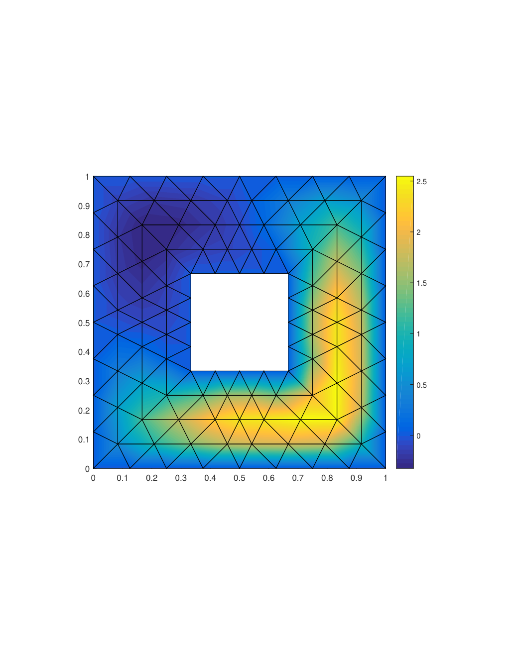
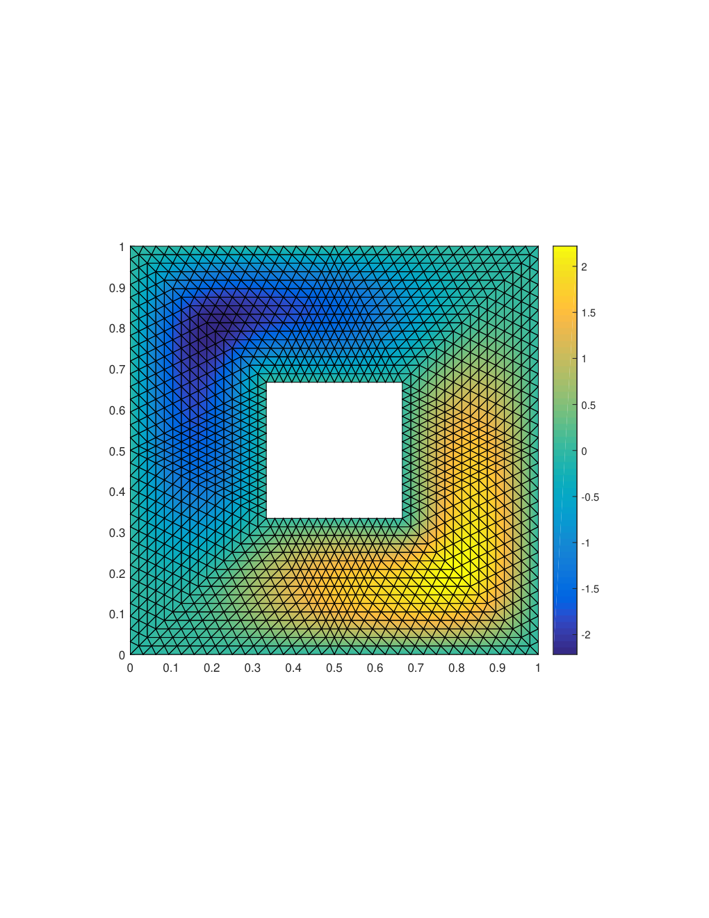
Finally, we consider the square ring $\Omega=(0,1)^{2}\setminus([1/3,2/3]^{2})$ . In this experiment, we use quasi-uniform meshes. The initial mesh on this domain is shown in Figure 1(c), and we refine the initial mesh uniformly to obtain finer meshes. The numerical eigenvalues and related convergence history are reported in Tables 7 and 8, respectively. It can be seen from Table 8 that despite the four re-entrant corners all numerical eigenvalues converge at the optimal rate $\mathcal{O}(h^{2})$ . Note that the convergence rate is better than what we obtained in Theorem 3.4. In Table 9, we display numerical results of five different methods on a quasi-uniform mesh with mesh size $\approx 0.0039.$ It can be seen that the performance of the modified mixed method is comparable to the $C^{0}$ IPG method, the Argyris method and the Morley method. In addtion, comparing with the usual mixed method, our method does not generate spurious eigenvalues.

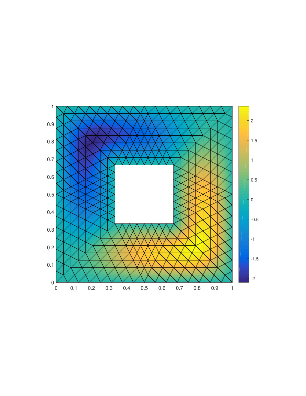
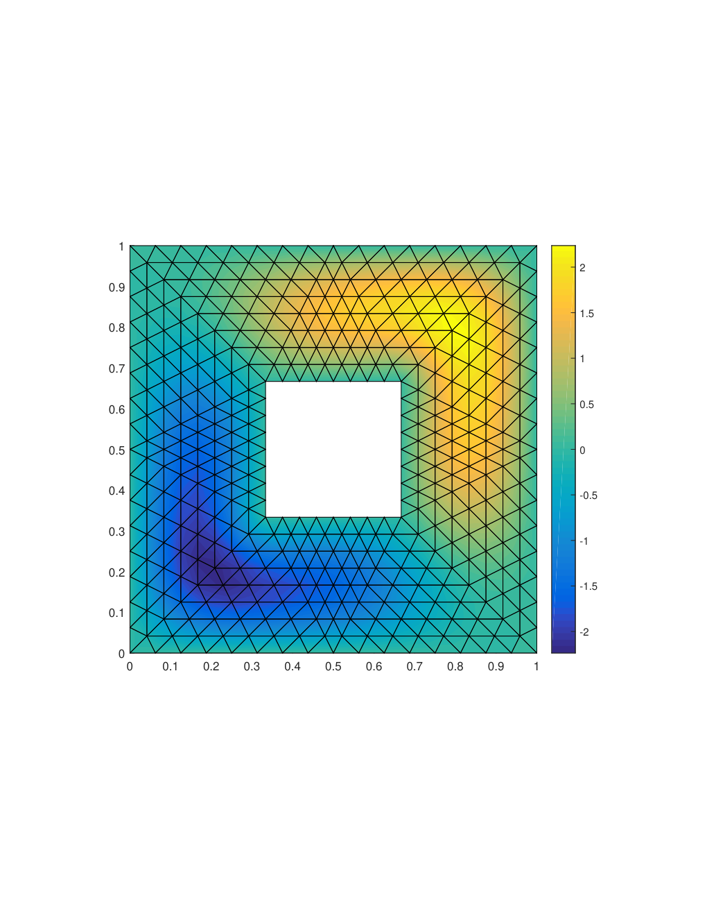
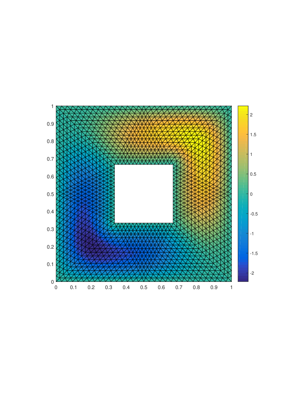
It worth mentioning that our method has certain advantages in approximating multiple eigenvalues. In this experiment, the second and the third eigenvalues are repeated, i.e. $\lambda_{2}=\lambda_{3}.$ The corresponding eigenfunctions are depicted in Figure 2. It can be seen that the second eigenfunction has singularities at the upper-left and low-right of the hole, while the third eigenfunction is singular at the other two opposite corners. To capture the singularities, a popular way is to use adaptive scheme. Several studies have shown that an effective adaptive strategy for multiple eigenvalues should consider all involved discrete eigenfunctions[3, 17, 9], otherwise the singularities of the target eigenfunctions may be resolved in a wrong way. However, the main issue is that in general it is not known a priori the multiplicity of an eigenvalue of the continuous problem, which in turn brings difficulties to the design of efficient adaptive methods.

Interestingly, it seems that our method does not need to consider these problems. As mentioned before, our method enjoys $\mathcal{O}(h^{2})$ convergence rate for the first six eigenvalues on quasi-uniform meshes, which means that there is no need to use adaptive method. Therefore, we do not need to bother to design efficient adaptive strategies, especially when the multiplicity of an eigenvalue is not known a priori. Moreover, due to the symmetry of the initial mesh and the uniform refinement strategy, numerical eigenvalues which approximate a multiple eigenvalue can be very close. For instance $\lambda_{2,h}$ and $\lambda_{3,h}$ in Table 7 are almost equal as $h\rightarrow 0$ . To sum up, our method has some potential in calculating multiple eigenvalues.

Table 7: The first six eigenvalues obtained by modified mixed method on the square ring.

dof	$\lambda_{1,h}$	$\lambda_{2,h}$	$\lambda_{3,h}$	$\lambda_{4,h}$	$\lambda_{5,h}$	$\lambda_{6,h}$
72	13199.3873	15043.5260	15221.0294	16069.9131	19530.5875	26203.3113
336	11833.8354	12463.7720	12536.8434	14675.5949	16125.1736	22760.3983
1440	11618.2080	12247.8454	12248.3350	14321.0590	15722.7245	21997.2147
5952	11586.6967	12204.9675	12204.9747	14231.2062	15644.8961	21808.1987
24192	11578.4400	12193.8534	12193.8536	14208.5011	15625.2749	21760.9347
97536	11576.3175	12191.0105	12191.0105	14202.7829	15620.2472	21749.0480
391680	11575.7742	12190.2890	12190.2890	14201.3466	15618.9871	21746.0760
1569792	11575.6342	12190.1048	12190.1048	14200.9864	15618.6663	21745.3307
6285312	11575.5987	12190.0583	12190.0583	14200.8962	15618.5853	21745.1440

Table 8: The convergence history of the first six eigenvalues in the square ring.

$h$	$\|\lambda_{1,h_{l+1}}-\lambda_{1,h_{l}}\|$	$\mathcal{R}$	$\|\lambda_{2,h_{l+1}}-\lambda_{2,h_{l}}\|$	$\mathcal{R}$	$\|\lambda_{3,h_{l+1}}-\lambda_{3,h_{l}}\|$	$\mathcal{R}$	$\|\lambda_{4,h_{l+1}}-\lambda_{4,h_{l}}\|$	$\mathcal{R}$	$\|\lambda_{5,h_{l+1}}-\lambda_{5,h_{l}}\|$	$\mathcal{R}$	$\|\lambda_{6,h_{l+1}}-\lambda_{6,h_{l}}\|$	$\mathcal{R}$
0.1250	1.366e+03		2.580e+03		2.684e+03		1.394e+03		3.405e+03		3.443e+03
0.0625	2.156e+02	2.66	2.159e+02	3.58	2.885e+02	3.22	3.545e+02	1.98	4.024e+02	3.08	7.632e+02	2.17
0.0313	3.151e+01	2.77	4.288e+01	2.33	4.336e+01	2.73	8.985e+01	1.98	7.783e+01	2.37	1.890e+02	2.01
0.0156	8.257e+00	1.93	1.111e+01	1.95	1.112e+01	1.96	2.271e+01	1.98	1.962e+01	1.99	4.726e+01	2.00
0.0078	2.122e+00	1.96	2.843e+00	1.97	2.843e+00	1.97	5.718e+00	1.99	5.028e+00	1.96	1.189e+01	1.99
0.0039	5.433e-01	1.97	7.215e-01	1.98	7.215e-01	1.98	1.436e+00	1.99	1.260e+00	2.00	2.972e+00	2.00
0.0020	1.400e-01	1.96	1.842e-01	1.97	1.842e-01	1.97	3.602e-01	2.00	3.207e-01	1.97	7.453e-01	2.00
0.0010	3.546e-02	1.98	4.650e-02	1.99	4.650e-02	1.99	9.022e-02	2.00	8.102e-02	1.98	1.867e-01	2.00

Table 9: The first six eigenvalues obtained by five methods on the square ring.

	dof	$\lambda_{1,h}$	$\lambda_{2,h}$	$\lambda_{3,h}$	$\lambda_{4,h}$	$\lambda_{5,h}$	$\lambda_{6,h}$
Modified Mixed	97536	11576.318	12191.010	12191.010	14202.783	15620.247	21749.048
$C^{0}$ IPG	391680	11936.788	12541.947	12541.947	14484.496	15993.189	21995.884
Argyris	885488	11771.381	12391.618	12391.618	14411.874	15819.480	21914.541
Morley	393216	10950.898	11651.220	11651.220	14105.090	14971.428	21571.899
Mixed	97536	6008.641	7149.365	7149.365	9659.918	14202.783	21052.856

Refer to caption — Figure 2: The eigenfunctions corresponding to $\lambda_{2}$ (left) and $\lambda_{3}$ (right) on the square ring for the three refinement levels

Acknowledgments

The authors would like to thanks anonymous referees for their valuable comments. This work is supported in part by the National Natural Science Foundation of China grants NSFC 11871092 and NSAF U1930402.

References

[1] I. Babuška and J. Osborn. Eigenvalue problems. In Handbook of numerical analysis, Vol. II, Handb. Numer. Anal., II, pages 641–787. North-Holland, Amsterdam, 1991.
[2] D. Boffi. Finite element approximation of eigenvalue problems. Acta Numer., 19:1–120, 2010.
[3] D. Boffi, R. G. Durán, F. Gardini, and L. Gastaldi. A posteriori error analysis for nonconforming approximation of multiple eigenvalues. Math. Methods Appl. Sci., 40(2):350–369, 2017.
[4] S. C. Brenner, P. Monk, and J. Sun. $C^{0}$ interior penalty Galerkin method for biharmonic eigenvalue problems. In Spectral and high order methods for partial differential equations—ICOSAHOM 2014, volume 106 of Lect. Notes Comput. Sci. Eng., pages 3–15. Springer, Cham, 2015.
[5] S. C. Brenner and L.-Y. Sung. $C^{0}$ interior penalty methods for fourth order elliptic boundary value problems on polygonal domains. J. Sci. Comput., 22/23:83–118, 2005.
[6] F. Chatelin. Spectral approximation of linear operators, volume 65 of Classics in Applied Mathematics. Society for Industrial and Applied Mathematics (SIAM), Philadelphia, PA, 2011.
[7] L. Chen. ifem: an innovative finite element methods package in matlab. Preprint, University of Maryland, 2008.
[8] P. G. Ciarlet and P.-A. Raviart. A mixed finite element method for the biharmonic equation. In Mathematical aspects of finite elements in partial differential equations (Proc. Sympos., Math. Res. Center, Univ. Wisconsin, Madison, Wis., 1974), pages 125–145. Publication No. 33, 1974.
[9] X. Dai, J. Xu, and A. Zhou. Convergence and optimal complexity of adaptive finite element eigenvalue computations. Numer. Math., 110(3):313–355, 2008.
[10] E. H. Georgoulis and P. Houston. Discontinuous Galerkin methods for the biharmonic problem. IMA J. Numer. Anal., 29(3):573–594, 2009.
[11] T. Gerasimov, A. Stylianou, and G. Sweers. Corners give problems when decoupling fourth order equations into second order systems. SIAM J. Numer. Anal., 50(3):1604–1623, 2012.
[12] P. Grisvard. Elliptic problems in nonsmooth domains, volume 24 of Monographs and Studies in Mathematics. Pitman (Advanced Publishing Program), Boston, MA, 1985.
[13] H. Li, P. Yin, and Z. Zhang. A ${C}^{0}$ finite element method for the biharmonic problem with Navier boundary conditions in a polygonal domain. arXiv preprint arXiv:2012.12374, 2020.
[14] L. Morley. The triangular equilibrium element in the solution of plate bending problems. Aeronaut, 19:149–169, 1968.
[15] I. Mozolevski, E. Süli, and P. R. Bösing. $hp$ -version a priori error analysis of interior penalty discontinuous Galerkin finite element approximations to the biharmonic equation. J. Sci. Comput., 30(3):465–491, 2007.
[16] S. A. Nazarov and G. Sweers. A hinged plate equation and iterated Dirichlet Laplace operator on domains with concave corners. J. Differential Equations, 233(1):151–180, 2007.
[17] P. Solin and S. Giani. An iterative adaptive finite element method for elliptic eigenvalue problems. J. Comput. Appl. Math., 236(18):4582–4599, 2012.
[18] Y. Yang, H. Bi, and Y. Zhang. The adaptive Ciarlet-Raviart mixed method for biharmonic problems with simply supported boundary condition. Appl. Math. Comput., 339:206–219, 2018.
[19] S. Zhang and Z. Zhang. Invalidity of decoupling a biharmonic equation to two Poisson equations on non-convex polygons. Int. J. Numer. Anal. Model., 5(1):73–76, 2008.

$\displaystyle\\|\rho-\rho_{h}\\|_{1}$	$\displaystyle\lesssim\\|\nabla(\rho-\mathcal{P}_{h}\rho)\\|_{0},$	(3.1)
$\displaystyle\\|\rho-\rho_{h}\\|_{0}$	$\displaystyle\lesssim\eta_{0}(h)\\|\nabla(\rho-\rho_{h})\\|_{0},$	(3.2)
$\displaystyle\\|\phi-\phi_{h}\\|_{1}$	$\displaystyle\lesssim\\|\phi-\mathcal{P}_{h}\phi\\|_{1}+\\|\rho-\rho_{h}\\|_{0}+\\|\xi-\xi_{h}\\|_{0},$	(3.3)
$\displaystyle\\|\phi-\phi_{h}\\|_{0}$	$\displaystyle\lesssim\eta_{0}(h)\\|\phi-\mathcal{P}_{h}\phi\\|_{1}+\\|\rho-\rho_{h}\\|_{0}+\\|\xi-\xi_{h}\\|_{0}.$	(3.4)

	$\displaystyle\\|\phi-\phi_{h}\\|_{s}$	$\displaystyle=\\|S(\rho-c(\rho)\xi)-S_{h}(\rho_{h}-c_{h}(\rho_{h})\xi_{h})\\|_{s}$
		$\displaystyle\leq\\|S(\rho-c(\rho)\xi)-S_{h}(\rho-c(\rho)\xi)\\|_{s}+\\|S_{h}(\rho-c(\rho)\xi)-S_{h}(\rho_{h}-c_{h}(\rho_{h})\xi_{h})\\|_{s}$
		$\displaystyle\leq\\|S(\rho-c(\rho)\xi)-\mathcal{P}_{h}S(\rho-c(\rho)\xi)\\|_{s}+\\|\rho-\rho_{h}\\|_{0}+\\|c(\rho)\xi-c_{h}(\rho_{h})\xi_{h}\\|_{0}$
		$\displaystyle\leq\\|\phi-\mathcal{P}_{h}\phi\\|_{s}+\\|\rho-\rho_{h}\\|_{0}+\\|c(\rho)(\xi-\xi_{h})\\|_{0}+\|c(\rho)-c_{h}(\rho_{h})\|\\|\xi_{h}\\|_{0}.$

$\displaystyle\|\lambda-\lambda_{h}\|$	$\displaystyle\lesssim\eta_{0}(h)(\\|u-\mathcal{P}_{h}u\\|_{1}+\\|\sigma-\mathcal{P}_{h}\sigma\\|_{1})+\\|\xi-\xi_{h}\\|_{0},$	(3.10)
$\displaystyle\\|u-u_{h}\\|_{0}$	$\displaystyle\lesssim\eta_{0}(h)(\\|u-\mathcal{P}_{h}u\\|_{1}+\\|\sigma-\mathcal{P}_{h}\sigma\\|_{1})+\\|\xi-\xi_{h}\\|_{0},$	(3.11)
$\displaystyle\\|u-u_{h}\\|_{1}$	$\displaystyle\lesssim\\|u-\mathcal{P}_{h}u\\|_{1}+\\|\sigma-\mathcal{P}_{h}\sigma\\|_{0}+\\|\xi-\xi_{h}\\|_{0},$	(3.12)
$\displaystyle\\|\sigma-\sigma_{h}\\|_{0}$	$\displaystyle\lesssim\eta_{0}(h)(\\|u-\mathcal{P}_{h}u\\|_{1}+\\|\sigma-\mathcal{P}_{h}\sigma\\|_{1})+\\|\xi-\xi_{h}\\|_{0},$	(3.13)
$\displaystyle\\|\sigma-\sigma_{h}\\|_{1}$	$\displaystyle\lesssim\eta_{0}(h)\\|u-\mathcal{P}_{h}u\\|_{1}+\\|\sigma-\mathcal{P}_{h}\sigma\\|_{1}+\\|\xi-\xi_{h}\\|_{0}.$	(3.14)

	$\displaystyle\\|Tf-T_{h}f\\|_{1}$	$\displaystyle\lesssim h\\|f\\|_{0},$		(3.15)
	$\displaystyle\\|Tf-T_{h}f\\|_{0}$	$\displaystyle\lesssim h^{2\alpha}\\|f\\|_{0}.$		(3.16)

$\displaystyle\lambda\\|(T-T_{h})u\\|_{0}$	$\displaystyle\lesssim\eta_{0}(h)\\|T(\lambda u)-\mathcal{P}_{h}T(\lambda u)\\|_{1}+\\|S(\lambda u)-S_{h}(\lambda u)\\|_{0}+\\|\xi-\xi_{h}\\|_{0}$
	$\displaystyle\lesssim\eta_{0}(h)\\|u-\mathcal{P}_{h}u\\|_{1}+\\|\sigma-\mathcal{P}_{h}\sigma\\|_{0}+\\|\xi-\xi_{h}\\|_{0}$
	$\displaystyle\lesssim\eta_{0}(h)(\\|u-\mathcal{P}_{h}u\\|_{1}+\\|\sigma-\mathcal{P}_{h}\sigma\\|_{1})+\\|\xi-\xi_{h}\\|_{0}.$	(3.19)