Exploring multi-Higgs models with softly broken large discrete symmetry groups

Numerous pieces of evidence suggest that the Standard Model (SM) cannot be the ultimate theoretical construction of the microscopic world. In the absence of direct compelling hints of how New Physics beyond the SM should look like, theorists explore different venues. A very active direction of research is the study of non-minimal scalar sectors, for a selection of topics see the recent reviews [1, 2, 3, 4]. The simple idea that Higgs doublets can come in generations, just like fermions, alleviates some of the problems of the SM and also leads to a surprisingly rich list of phenomena. After a decades-long study of the two-Higgs-doublet models (2HDMs) [1], the community is exploring other scalar sectors, such as the three-Higgs-doublet models (3HDMs).

First proposed by S. Weinberg in 1976 [5], the 3HDMs equipped with various global symmetries, exact or softly broken, were studied in hundreds of papers, see a brief historical overview in [3]. However, a systematic study of all the opportunities offered by the 3HDMs is still lacking. One obvious reason for that is the very large number of free parameters. The most general renormalizable scalar potential of the $N$-Higgs-doublet model can be written, at the tree level, as

$$V=Y_{ij}(\phi^{\dagger}_{i}\phi_{j})+Z_{ijkl}(\phi^{\dagger}_{i}\phi_{j})(\phi^{\dagger}_{k}\phi_{l})\,,\quad i,j,k,l=1,\dots,N,$$

(1)

with 54 free parameters for $N=3$. If one includes the quark Yukawa sector, the total number of free parameters exceeds one hundred. Certainly, it is possible, for any particular point in the entire parameter space, to numerically minimize the potential, compute all scalar masses and couplings, track down the fermion sector and its interaction with new scalars. But the real challenge is to make sense of these case-by-case calculations and to identify all the essentially distinct phenomenological situations which may be hiding in various parts of the very-large-dimensional parameter space. The richness of the 3HDM is just too vast to grasp and visualize with a straightforward (numerical) approach.

One popular way to tame the proliferation of free parameters is to assume that the multi-Higgs model is equipped with an additional global symmetry group. In early 1980’s, this approach seemed promising because one hoped to link the mixing angles of the Cabibbo-Kobayashi-Maskawa matrix with quark mass ratios [3]. Later it turned out that this direct approach exploiting the exact symmetry groups could not lead to a viable quark sector [6, 7], but softly broken symmetries seemed to offer sufficient flexibility and interesting predictions. In the case of the 3HDM scalar sector, several continuous and discrete symmetry groups have been implemented, starting from Weinberg’s model, which has the symmetry group $\mathbb{Z}_{2}\times\mathbb{Z}_{2}$. The full classification of discrete symmetry groups usable in the scalar sector of the 3HDM was established in [8]. If one focuses on the Higgs potential alone, one can observe accidental symmetries which go beyond Higgs family transformations. They were classified in [9] and a deeper analysis of the so-called maximally symmetric 3HDM was presented in [10]. The full list of symmetry groups suitable for the 3HDM Yukawa sector is still not known. The $CP$ properties of the 3HDM scalar sector were also explored by using basis-independent methods [11, 12, 13, 14, 15].

Investigation of the 3HDMs with softly broken global symmetry group $G$ depends on the group itself. Let us focus on the attractive case of large discrete groups $G$, with Higgs doublets transforming as an irreducible triplet representations. Four such cases are known¹¹ 1 The 3HDM with a $\Delta(27)$ triplet leads to the same potential as the potential for a $\Delta(54)$ group, so it is implicitly included in the $\Delta(54)$ case. [8]: $G=A_{4}$, $S_{4}$, $\Delta(54)$, and $\Sigma(36)$-symmetric 3HDMs. In any of these four cases, the Higgs potential invariant under $G$ has the following form:

$$V_{0}=-m^{2}(\phi_{1}^{\dagger}\phi_{1}+\phi_{2}^{\dagger}\phi_{2}+\phi_{3}^{\dagger}\phi_{3})+V_{4}\,,$$

(2)

while the $G$-symmetric quartic potential $V_{4}$ contains several terms. All possible minima of this potential for the symmetry groups $A_{4}$, $S_{4}$, $\Delta(54)$, and $\Sigma(36)$ are known and were put together in [16] (see also [17]).

If one wants to explore a 3HDM with a softly broken group $G$, one needs to introduce all possible quadratic terms:

$\displaystyle V_{\rm soft}=m_{11}^{2}\phi_{1}^{\dagger}\phi_{1}+m_{22}^{2}\phi_{2}^{\dagger}\phi_{2}+m_{33}^{2}\phi_{3}^{\dagger}\phi_{3}+\left(m_{12}^{2}\,\phi_{1}^{\dagger}\phi_{2}+m_{23}^{2}\,\phi_{2}^{\dagger}\phi_{3}+m_{31}^{2}\,\phi_{3}^{\dagger}\phi_{1}+h.c.\right)$

(3)

with complex $m_{ij}^{2}$ for $i\not=j$. In total, there are nine free parameters here. Exploring in detail the emerging phenomenology in all corners of this 9-dimensional soft breaking parameter space and visualizing the results would be very challenging. However these free parameters do not play equal roles. Some parameters may trigger structural changes, while others will only shift the numerical values of the observables. Some phenomena may happen along generic directions in this soft breaking parameter space, while other effects may take place only along some very particular directions. One could even think of plotting a phase diagram of the phenomenology of the resulting 3HDM with softly broken $G$, but describing it in its full dimensionality seems very hard.

In short, one needs a guiding principle and a set of efficient methods to make sense of multi-Higgs models with softly broken large discrete symmetry groups.

This is the main goal of the present paper. We will show that the nine soft breaking free parameters can be split into two families: five parameters which preserve the vacuum expectation value (vev) alignment of the exactly symmetric parent model, and the four parameters which drive this alignment away in four orthogonal directions. Focusing on the vev-preserving parameters, we will show which structural features of the fully symmetric model stay unchanged and which get modified, and how to track the effect of each of these parameters. In particular, we will find that, although the models with vev-preserving soft breaking terms do not possess any exact symmetry, their scalar sector phenomenology “inherits” some of the features from the parent $G$-symmetric model. These results help develop qualitative and quantitative intuition when building multi-Higgs models with softly broken large discrete symmetry groups.

These phenomena will be illustrated with the example of the largest discrete symmetry group possible in the 3HDM scalar sector, the group $\Sigma(36)$, which is not as well known as the $A_{4}$, $S_{4}$, or $\Delta(54)$-symmetric 3HDMs. The application of the methodology developed here to those groups and the inclusion of the Yukawa sector are delegated to future works.

The structure of the paper is the following. In the next section we outline the properties of the scalar sector emerging in the $\Sigma(36)$-symmetric 3HDM. In section 3 we construct the soft breaking terms which preserve any chosen vev alignment of the symmetric model and illustrate the general procedure with the softly broken $\Sigma(36)$ 3HDM. Finally, we discuss the results and draw conclusions, while the Appendix provide auxiliary mathematical details.

$\Sigma(36)$ is the largest discrete symmetry group which can be imposed on the scalar sector of the 3HDM without leading to accidental continuous symmetries [8]. Group-theoretically, it is defined as a $\mathbb{Z}_{4}$ permutation acting on generators of the abelian group $\mathbb{Z}_{3}\times\mathbb{Z}_{3}$:

$$\Sigma(36)\simeq(\mathbb{Z}_{3}\times\mathbb{Z}_{3})\rtimes\mathbb{Z}_{4}\,.$$

(4)

The generators of the $\mathbb{Z}_{3}\times\mathbb{Z}_{3}$ “core” and the generator of $\mathbb{Z}_{4}$ are

$$a=\begin{pmatrix}1&0&0\\ 0&\omega&0\\ 0&0&\omega^{2}\end{pmatrix}\,,\quad b=\begin{pmatrix}0&1&0\\ 0&0&1\\ 1&0&0\end{pmatrix}\,,\quad d={i\over\sqrt{3}}\left(\begin{array}[]{ccc}1&1&1\\ 1&\omega^{2}&\omega\\ 1&\omega&\omega^{2}\end{array}\right)\,,$$

(5)

where $\omega=\exp(2\pi i/3)$. The orders of these generators are:

$$a^{3}={\boldsymbol{1}}\,,\quad b^{3}={\boldsymbol{1}}\,,\quad d^{4}={\boldsymbol{1}}\,.$$

Notice that $d^{2}$ is a transformation which transposes two doublets; thus, $\Sigma(36)$ contains all permutations of the three doublets. Had we imposed symmetry under $d^{2}$ but not $d$, we would end up with the more familiar symmetry group $\Delta(54)$, first used within the 3HDMs back in late 1970’s [18] and explored later in [19, 20, 21, 22]. For more details on the relation between $\Delta(54)$ and $\Sigma(36)$ and the subtleties of their definitions, see Appendix A.

The scalar potential of 3HDM invariant under $\Sigma(36)$ has the following form:

	$\displaystyle V_{0}$	$\displaystyle=$	$\displaystyle-m^{2}\left[\phi_{1}^{\dagger}\phi_{1}+\phi_{2}^{\dagger}\phi_{2}+\phi_{3}^{\dagger}\phi_{3}\right]+\lambda_{1}\left[\phi_{1}^{\dagger}\phi_{1}+\phi_{2}^{\dagger}\phi_{2}+\phi_{3}^{\dagger}\phi_{3}\right]^{2}$		(6)
			$\displaystyle-\lambda_{2}\left[|\phi_{1}^{\dagger}\phi_{2}|^{2}+|\phi_{2}^{\dagger}\phi_{3}|^{2}+|\phi_{3}^{\dagger}\phi_{1}|^{2}-(\phi_{1}^{\dagger}\phi_{1})(\phi_{2}^{\dagger}\phi_{2})-(\phi_{2}^{\dagger}\phi_{2})(\phi_{3}^{\dagger}\phi_{3})-(\phi_{3}^{\dagger}\phi_{3})(\phi_{1}^{\dagger}\phi_{1})\right]$
			$\displaystyle+\lambda_{3}\left(|\phi_{1}^{\dagger}\phi_{2}-\phi_{2}^{\dagger}\phi_{3}|^{2}+|\phi_{2}^{\dagger}\phi_{3}-\phi_{3}^{\dagger}\phi_{1}|^{2}+|\phi_{3}^{\dagger}\phi_{1}-\phi_{1}^{\dagger}\phi_{2}|^{2}\right)\,.$

It has four real free parameters. The first two lines of Eq. (6) are invariant under the entire $SU(3)$ transformation group of the three Higgs doublets. The positive sign of $\lambda_{2}$ guarantees that the minimum corresponds to a neutral vacuum, but the minimization of these two lines alone would lead to several neutral Nambu-Goldstone bosons. The last term with the coefficient $\lambda_{3}$ selects the discrete $\Sigma(36)$ group out of it and renders those Higgs bosons massive.

The potential of Eq. (6) is also $CP$ invariant. Apart from the standard $CP$ symmetry $\phi_{i}\mapsto\phi_{i}^{*}$, it is also invariant under many other $CP$ transformations of the form of the standard $CP$ combined with any of the symmetries from $\Sigma(36)$. Unlike the $\Delta(54)$ 3HDM, the absence of $CP$ violation in $\Sigma(36)$ 3HDM is not an assumption but is a consequence of the $\mathbb{Z}_{4}$ subgroup which forbids any form of $CP$ violation in 3HDM, explicit or spontaneous [23, 16].

An important feature of the entire $\Delta(54)$ family of 3HDM models, including $\Sigma(36)$ 3HDM, is the rigid structure of its minima. Depending on the values of the parameters, the global minimum of the potential can only correspond to the following vev alignments [16]:

	alignment $A$:		$\displaystyle A_{1}=(\omega,\,1,\,1)\,,\quad A_{2}=(1,\,\omega,\,1),\,\quad A_{3}=(1,\,1,\,\omega)$		(7)
	alignment $A^{\prime}$:		$\displaystyle A^{\prime}_{1}=(\omega^{2},\,1,\,1)\,,\quad A^{\prime}_{2}=(1,\,\omega^{2},\,1),\,\quad A^{\prime}_{3}=(1,\,1,\,\omega^{2})$		(8)
	alignment $B$:		$\displaystyle B_{1}=(1,\,0,\,0)\,,\quad B_{2}=(0,\,1,\,0),\,\quad B_{3}=(0,\,0,\,1)$		(9)
	alignment $C$:		$\displaystyle C_{1}=(1,\,1,\,1)\,,\quad C_{2}=(1,\,\omega,\,\omega^{2})\,,\quad C_{3}=(1,\,\omega^{2},\,\omega)$		(10)

Notice that, due to the global symmetry of the 3HDM potential under simultaneous phase rotation of the three doublets, other possible configurations can be reduced to these ones; for example, $(\omega,\,\omega^{2},\,1)=\omega(1,\,\omega,\,\omega^{2})$ also corresponds to the alignment $C_{2}$. The phase rigidity is reflected in the fact that the relative phases between vevs are calculable and are not sensitive to the exact numerical values of the coefficients. This rigidity was behind the “geometric $CP$-violation” proposal back in 1984 [24] which was revisited in more detail in [25, 26, 27], and also shown to be compatible with viable Yukawa sectors [28, 29, 30].

None of the minima of the $\Sigma(36)$-symmetric 3HDM breaks the symmetry group completely [16]. There are six family symmetries and six $CP$-type symmetries which are preserved at each vev alignment. Other, spontaneously broken, symmetries link different vacua, which, despite looking differently, represent the same physics. For $\lambda_{3}<0$, the global minima are at the six points $A$ and $A^{\prime}$, which are related by the broken symmetries from $\Sigma(36)$. For $\lambda_{3}>0$, the degenerate global minima are at points $B$ or $C$. Thus, we have two essentially distinct phenomenological situations in $\Sigma(36)$ 3HDM.

Further insights into the structural properties of the model, including the vev alignments, symmetry and $CP$ properties, can be gained if one pays attention not only to the transformations from the symmetry group $G$ but also to the transformations from $SU(3)$ which leave $G$ invariant, or “symmetries of symmetries” in the language of [31]. The potential remains form-invariant under such transformations, only up to reparametrizatioon of coefficients, which may provide additional links between different regimes of the same model.

Three Higgs doublets contain 12 real fields. When expanding the potential around a neutral vacuum, one absorbs, as usual, three of them in the longitudinal components of the $W^{\pm}$ and $Z$-bosons. What remains is two pairs of charged Higgses and five neutral Higgs bosons. At points $B$ or $C$, the Higgs boson masses are

	$\displaystyle m_{h_{SM}}^{2}$	$\displaystyle=$	$\displaystyle 2\lambda_{1}v^{2}=2m^{2}\,,$
	$\displaystyle m_{H^{\pm}}^{2}$	$\displaystyle=$	$\displaystyle{1\over 2}\lambda_{2}v^{2}\quad\mbox{(double degenerate)}\,,$
	$\displaystyle m_{h}^{2}$	$\displaystyle=$	$\displaystyle{1\over 2}\lambda_{3}v^{2}\quad\mbox{(double degenerate)}\,,$
	$\displaystyle m_{H}^{2}$	$\displaystyle=$	$\displaystyle 3m_{h}^{2}={3\over 2}\lambda_{3}v^{2}\quad\mbox{(double degenerate)}\,.$		(11)

At points $A$ and $A^{\prime}$, which are the minima for $\lambda_{3}<0$, the Higgs masses are

	$\displaystyle m_{h_{SM}}^{2}$	$\displaystyle=$	$\displaystyle 2(\lambda_{1}+\lambda_{3})v^{2}=2m^{2}\,,$
	$\displaystyle m_{H^{\pm}}^{2}$	$\displaystyle=$	$\displaystyle{1\over 2}(\lambda_{2}-3\lambda_{3})v^{2}\quad\mbox{(double degenerate)}\,,$
	$\displaystyle m_{h}^{2}$	$\displaystyle=$	$\displaystyle-{1\over 2}\lambda_{3}v^{2}\quad\mbox{(double degenerate)}\,,$
	$\displaystyle m_{H}^{2}$	$\displaystyle=$	$\displaystyle 3m_{h}^{2}=-{3\over 2}\lambda_{3}v^{2}\quad\mbox{(double degenerate)}\,.$		(12)

Identification of the SM-like Higgs boson is unambiguous. It is a straightforward exercise to show that, if the quadratic potential of an NHDM has the form $m^{2}\sum_{i}\phi_{i}^{\dagger}\phi_{i}$, then whatever the quartic potential is, the model automatically incorporates the exact scalar alignment [32]. This means that the direction along the vev alignment is a mass eigenstate which, therefore, couples to the $WW$ and $ZZ$ pairs just as in the SM. The other neutral Higgs bosons do not couple to gauge-boson pairs.

The fact that the symmetry group $\Sigma(36)$ is not broken completely by the vacuum configuration means that one can classify the physical Higgs bosons according to their conserved charges. For example, the vev alignment $(1,0,0)$ corresponding to point $B$ preserves the symmetry group $S_{3}$ generated by $a$ and $d^{2}$. Thus, within each subspace of physical scalar fields (the charged, the light neutral, and the heavy neutral Higgses) we can construct states which are eigenstates of parity under $d^{2}$ or which have definite $Z_{3}$-charges under $a$. Either of these numbers is conserved. Thus, the lightest pair of states from the second and third doublet is stable against decay to the SM fields (provided they do not couple to fermions).

To summarize the above observations, we list here the structural features of the $\Sigma(36)$-symmetric 3HDM scalar sector.

• •

  The vev alignment at the global minimum can only be of types (7) to (10).

• •

  Spontaneous $CP$ violation is impossible.

• •

  The model contains automatic scalar alignment, with the SM-like Higgs $h_{SM}$.

• •

  All charged Higgses are degenerate, and the four non-SM-like neutral Higgs bosons are pair-wise degenerate.

• •

  The masses of the two pairs of the neutral Higgses are related as $m_{H}^{2}=3m_{h}^{2}$.

• •

  Since the full symmetry group $\Sigma(36)$ is broken only partially at any of the vev alignments, the lightest non-SM-like Higgs bosons are stable against decay to the SM fields.

Suppose we pick up one of the vev alignments listed in Eqs. (7) through (10). Which terms in $V_{\rm soft}$ can we introduce to keep the alignment intact?

A straightforward way to answer this question for all alignments, one by one, is to write down the extremum conditions, solve them and deduce the relations among the parameters $m_{ij}^{2}$ which protect the chosen vev alignment. This method is not very enlightening. First, it requires direct computations of derivatives for each individual case. Second, when it leads to certain constraints on the soft breaking parameters $m_{ij}^{2}$, it may remain obscure within what range one is allowed to vary them. Finally, there may arise particular points which may require special treatment.

Instead, we propose here a simple method which leads to a clear picture for any vev alignment. Furthermore, it can be applied not only to the $\Sigma(36)$ 3HDM, but to any multi-Higgs potential with the trivial quadratic part, which includes $A_{4}$, $S_{4}$ and $\Delta(54)$ 3HDMs.

First, we remind the reader that, when we have a function which depends on the complex variable $z$ and its conjugate $z^{*}$, we can differentiate it with respect to $z$ and $z^{*}$ independently. Writing $z=x+iy$, we define the antiholomorphic derivative operator as

$$\frac{\partial}{\partial z^{*}}=\frac{1}{2}\left(\frac{\partial}{\partial x}+i\frac{\partial}{\partial y}\right),\quad\frac{\partial z}{\partial z^{*}}=0\,,\quad\frac{\partial z^{*}}{\partial z^{*}}=1\,.$$

(13)

The $\Sigma(36)$-invariant potential $V_{0}=-m^{2}\phi_{i}^{\dagger}\phi_{i}+V_{4}$ depends on the complex variables $\phi_{i}$ and $\phi_{i}^{\dagger}$. Here, the index $i$ can run over six entries: three upper and three lower components of the doublets. However, since the minimum is neutral, one can suppress the upper components and assume that $\phi_{i}=\phi_{i}^{0}$, $i=1,2,3$.

The extremization condition for the $\Sigma(36)$-symmetric potential is:

$$\frac{\partial V_{0}}{\partial\phi_{i}^{*}}=-m^{2}\phi_{i}+\frac{\partial V_{4}}{\partial\phi_{i}^{*}}=0\,.$$

(14)

Therefore, at the extremum point, we have

$$\frac{\partial V_{4}}{\partial\phi_{i}^{*}}\Bigg|_{V_{0}\ \rm extremum}=m^{2}\phi_{i}\big|_{V_{0}\ \rm extremum}\,.$$

(15)

Now, we add the soft breaking terms of Eq. (3), which we write compactly as

$$V_{\rm soft}=\phi_{i}^{\dagger}M_{ij}\phi_{j}\,,\quad M_{ij}=\left(\!\!\begin{array}[]{ccc}m_{11}^{2}&m_{12}^{2}&(m_{31}^{2})^{*}\\ (m_{12}^{2})^{*}&m_{22}^{2}&m_{23}^{2}\\ m_{31}^{2}&(m_{23}^{2})^{*}&m_{33}^{2}\\ \end{array}\!\!\right)\,,$$

(16)

with hermitean matrix $M$. Extremization condition for the full potential $V=V_{0}+V_{\rm soft}$ is

$$\frac{\partial V}{\partial\phi_{i}^{*}}=M_{ij}\phi_{j}-m^{2}\phi_{i}+\frac{\partial V_{4}}{\partial\phi_{i}^{*}}=0\,.$$

(17)

In general, the extremum point may have shifted with respect to the symmetric case, so we cannot use the relation of Eq. (15). But we now require that the soft breaking terms preserve the vev alignment up to rescaling: $v|_{V\ \rm extremum}=\zeta\cdot v|_{V_{0}\ \rm extremum}$. Because of this feature and because the quadratic and quartic terms are homogeneous functions with degrees 2 and 4, respectively, we can now state that

$$\frac{\partial V_{4}}{\partial\phi_{i}^{*}}\Bigg|_{V\ \rm extremum}=\zeta^{2}\cdot m^{2}\phi_{i}\big|_{V\ \rm extremum}\,.$$

(18)

Therefore, at the point of the extremum of $V$ we can simplify Eq. (17) as

$$M_{ij}\phi_{j}=(1-\zeta^{2})m^{2}\phi_{i}\,.$$

(19)

We conclude that the soft breaking terms preserve a vev alignment of the original symmetric model if and only if this vev alignment is an eigenvector of the corresponding matrix $M$. This offers us a method of writing down the most general soft breaking terms which preserve any given vev alignment of the symmetric model.

Let us illustrate this method with point $C_{1}$ whose vev alignment is $(1,1,1)$. We want to establish the form of $M$ which would preserve this alignment. Suppose $\mu_{1}$, $\mu_{2}$, $\mu_{3}$ are the eigenvalues of $M$, and the complex vectors $\vec{n}_{1}$, $\vec{n}_{2}$, $\vec{n}_{3}$ are the corresponding orthonormal eigenvectors. Then $M$ can be written as

$$M_{ij}=\mu_{1}\,n_{1i}n^{*}_{1j}+\mu_{2}\,n_{2i}n^{*}_{2j}+\mu_{3}\,n_{3i}n^{*}_{3j}\,.$$

(20)

Given one eigenvector, which is already known,

$$n_{1}=\frac{1}{\sqrt{3}}\left(\!\begin{array}[]{c}1\\ 1\\ 1\end{array}\!\right)\,,$$

(21)

we can select two other eigenvectors in the subspace orthogonal to $\vec{n}_{1}$. Let us define two orthonormal vectors in this subspace, for example,

$$e_{2}=\frac{1}{\sqrt{2}}\left(\!\begin{array}[]{c}0\\ 1\\ -1\end{array}\!\right)\quad\mbox{and}\quad e_{3}=\frac{1}{\sqrt{6}}\left(\!\begin{array}[]{c}-2\\ 1\\ 1\end{array}\!\right)\,.$$

(22)

Both $\{\vec{n}_{2},\vec{n}_{3}\}$ and $\{\vec{e}_{2},\vec{e}_{3}\}$ form a basis. Therefore, the two eigenvectors $\vec{n}_{2}$ and $\vec{n}_{3}$ can be obtained from $\vec{e}_{2}$ and $\vec{e}_{3}$ with an appropriate unitary transformation within this space:

$$\vec{n}_{i}=\mathcal{U}_{ij}\vec{e}_{j}\,,\quad i,j=2,3,\quad\mbox{where}\quad\mathcal{U}=\begin{pmatrix}\cos\theta&e^{i\xi}\sin\theta\\ -e^{-i\xi}\sin\theta&\cos\theta\end{pmatrix}.$$

(23)

Notice that multiplying $\vec{n}_{2}$ and $\vec{n}_{3}$ with additional phase factors does not affect $M$. Thus, the most general soft breaking terms preserving the vev alignment of point $A$ are described with the matrix $M$ in Eq. (20) with the following free parameters:

$$\mu_{1}=m^{2}(1-\zeta^{2}),\quad\mu_{2},\quad\mu_{3},\quad\theta,\quad\xi\,.$$

(24)

If we insist not only on keeping the vev alignment, but also want to preserve the value of $v$, we set $\mu_{1}=0$ and are left with 4 parameters, which we recast in the following more convenient form:

$$\Sigma=\mu_{2}+\mu_{3}\,,\quad\delta=\mu_{2}-\mu_{3}\,,\quad\theta,\quad\xi\,.$$

(25)

All these parameters can vary in their full domains of definitions.

The explicit expressions for the matrix $M$ and individual $m_{ij}^{2}$ soft breaking parameters which preserve the vev alignment $C_{1}$ and the value of $v$ are

	$\displaystyle M_{11}$	$\displaystyle=$	$\displaystyle m_{11}^{2}=\frac{1}{3}\left(\Sigma-\delta\cos 2\theta\right)$
	$\displaystyle M_{22}$	$\displaystyle=$	$\displaystyle m_{22}^{2}=\frac{1}{3}\left[\Sigma+\delta\left(\frac{\sqrt{3}}{2}\sin 2\theta\cos\xi+\frac{1}{2}\cos 2\theta\right)\right]$
	$\displaystyle M_{33}$	$\displaystyle=$	$\displaystyle m_{22}^{2}=\frac{1}{3}\left[\Sigma+\delta\left(-\frac{\sqrt{3}}{2}\sin 2\theta\cos\xi+\frac{1}{2}\cos 2\theta\right)\right]$
	$\displaystyle M_{12}$	$\displaystyle=$	$\displaystyle m_{12}^{2}=\frac{1}{6}\left[-\Sigma+\delta(-\sqrt{3}\sin 2\theta e^{i\xi}+\cos 2\theta)\right]$
	$\displaystyle M_{31}$	$\displaystyle=$	$\displaystyle m_{31}^{2}=\frac{1}{6}\left[-\Sigma+\delta(\sqrt{3}\sin 2\theta e^{-i\xi}+\cos 2\theta)\right]$
	$\displaystyle M_{23}$	$\displaystyle=$	$\displaystyle m_{23}^{2}=\frac{1}{6}\left[-\Sigma-\delta(i\sqrt{3}\sin 2\theta\sin\xi+2\cos 2\theta)\right]\,.$		(26)

In a similar fashion, we parametrize the soft breaking terms which preserve all other vev alignments of the $\Sigma(36)$ 3HDM, see Appendix B for the full list. Here we only remark that, in each case, there exists ambiguity in choosing the basis vectors $\vec{e}_{2}$ and $\vec{e}_{3}$ with respect to which we parametrize the matrix $M_{ij}$ via angles $\theta$ and $\xi$. We resolve this ambiguity by choosing such vectors that the neutral physical Higgs boson masses to be given below take exactly the same form at all minima.

Parametrizing the vev-preserving soft breaking terms as outlined above, we computed in each case the mass matrices of the physical Higgs bosons. A remarkable observation is that for all vev alignments and with the above choices of the parametrization procedure, we could obtain universal formulas for masses of the physical Higgs bosons, valid for all the vev alignments of the parent $\Sigma(36)$-symmetric model.

• •

  The scalar alignment feature is preserved. Indeed, since the vev alignment was the eigenvector of the parent model at its minimum and since it is an eigenvector of the matrix of the soft breaking terms, it will remain an eigenvector of the Hessian matrix of the softly broken case.

• •

  Since we select $\mu_{1}=0$ to preserve not only the alignment but also the value of $v$, the mass of the SM-like Higgs boson is unchanged: $m^{2}_{h_{SM}}=2(\lambda_{1}+\lambda_{3})v^{2}$ for cases $A$ and $A^{\prime}$ and $m^{2}_{h_{SM}}=2\lambda_{1}v^{2}$ for cases $B$ and $C$, just as in Eqs. (12) and (11).

• •

  The non-standard Higgs bosons cease to be mass degenerate. For the charged Higgs bosons, we write $m^{2}_{H^{\pm}_{i}}=m^{2}_{H^{\pm}_{i}}\big|_{\Sigma(36)}+\Delta m^{2}_{H^{\pm}_{i}}$, where $m^{2}_{H^{\pm}_{i}}\big|_{\Sigma(36)}$ are their masses in the parent $\Sigma(36)$-symmetric model given by Eqs. (12) and (11), and observe the following universal corrections:

  $$\Delta m^{2}_{H^{\pm}_{1}}=\mu_{2}=\frac{\Sigma+\delta}{2},\quad\Delta m^{2}_{H^{\pm}_{2}}=\mu_{3}=\frac{\Sigma-\delta}{2}\,.$$

  (27)

  The four non-SM-like neutral Higgs bosons have the following masses:

  	$\displaystyle m^{2}_{h_{1}}$	$\displaystyle=$	$\displaystyle\frac{1}{2}\left(2\lvert\lambda_{3}\rvert v^{2}+\Sigma-\sqrt{(\lambda_{3}v^{2})^{2}+\delta^{2}+2x\lvert\lambda_{3}\rvert|\delta|v^{2}}\right),$		(28)
  	$\displaystyle m^{2}_{h_{2}}$	$\displaystyle=$	$\displaystyle\frac{1}{2}\left(2\lvert\lambda_{3}\rvert v^{2}+\Sigma-\sqrt{(\lambda_{3}v^{2})^{2}+\delta^{2}-2x\lvert\lambda_{3}\rvert|\delta|v^{2}}\right),$		(29)
  	$\displaystyle m^{2}_{H_{1}}$	$\displaystyle=$	$\displaystyle\frac{1}{2}\left(2\lvert\lambda_{3}\rvert v^{2}+\Sigma+\sqrt{(\lambda_{3}v^{2})^{2}+\delta^{2}-2x\lvert\lambda_{3}\rvert|\delta|v^{2}}\right),$		(30)
  	$\displaystyle m^{2}_{H_{2}}$	$\displaystyle=$	$\displaystyle\frac{1}{2}\left(2\lvert\lambda_{3}\rvert v^{2}+\Sigma+\sqrt{(\lambda_{3}v^{2})^{2}+\delta^{2}+2x\lvert\lambda_{3}\rvert|\delta|v^{2}}\right)\,,$		(31)

  where the quantity $x\in[0,1]$ is

  $$x=\sqrt{1-(\sin 2\theta\sin\xi)^{2}}\,.$$

  (32)

  Here, we write $\lvert\lambda_{3}\rvert$ to cover both cases $A$ and $A^{\prime}$ ($\lambda_{3}<0$) and cases $B$ and $C$ ($\lambda_{3}>0$).

Apart from splitting, the mass patterns demonstrate two remarkable features. The first is the unexpected similarity between the cases $A+A^{\prime}$ and $B+C$. Indeed, cases $A$ and $A^{\prime}$ are linked by a symmetry of the parent model, and therefore, one expects that the appropriately parametrized soft terms would lead to the same results for points $A$ and $A^{\prime}$. In a similar way, symmetries link cases $B$ and $C$. However, there is no symmetry of the model which links the vev alignments from points $A$ or $A^{\prime}$ to points $B$ or $C$. Indeed, we see that the expressions for the SM-like and charged Higgs masses are not identical. Whether this intriguing feature can be explained from the “symmetries of symmetries” perspective of [31] is an open question which deserves a closer look.

The second feature is that the masses depend not on four, but on three independent soft breaking parameters: $\Sigma$, $\delta$, and the combination $\sin 2\theta\sin\xi$. In the example of point $C$, this combination quantifies the imaginary part of $m_{ij}^{2}$ in Eq. (3.2). This means that, in the 4D space of vev-preserving soft breaking parameters, there exist lines of identical Higgs spectra. Moving along these lines, one can adjust additional features of the model, keeping the masses fixed.

It is interesting to observe that, at $\sin 2\theta\sin\xi=1$ leading to $x=0$, the four neutral Higgses again combine into two mass-degenerate pairs. The origin of this degeneracy is the special form of the soft breaking terms which satisfy $\sin 2\theta\sin\xi=1$. Such soft breaking terms, in fact, respect several of the symmetries of the vacuum. Within the same example $C_{1}$, the soft breaking matrix takes the form

$$M=\frac{\Sigma}{6}\left(\!\!\begin{array}[]{ccc}2&-1&-1\\ -1&2&-1\\ -1&-1&2\\ \end{array}\!\!\right)+\frac{\delta\sqrt{3}}{6}\left(\!\!\begin{array}[]{ccc}0&-i&i\\ i&0&-i\\ -i&i&0\\ \end{array}\!\!\right)\,,$$

(33)

which is invariant under cyclic permutations as well as an exchange of any two doublets followed by a $CP$ transformation. These residual symmetries form the group $S_{3}$ and force the neutral scalars to be pairwise degenerate.

The third observation is the remarkable form of neutral mass splittings:

$$m_{h_{2}}^{2}-m_{h_{1}}^{2}=m_{H_{2}}^{2}-m_{H_{1}}^{2}\,.$$

(34)

It can be viewed as yet another structural feature inherited from the parent symmetric model.

The potential of the parent $\Sigma(36)$-invariant 3HDM contains six distinct minima which are linked by the broken symmetry generators and are degenerate. When we introduce soft breaking terms, we destroy the symmetry, and the six minima are not equivalent anymore. Therefore, one can wonder if the minimum which one selects to construct the vev-preserving soft breaking terms represents the global or a local minimum. The answer turns out surprisingly simple: the chosen minimum remains the global one if $\mu_{2}>0$ and $\mu_{3}>0$. Additionally, we verified numerically and found that for negative, but small values of either $\mu_{2}$ or $\mu_{3}$, the minimum can remain global. The smallness can be quantified relative to the coefficient of the $SU(3)$-invariant quadratic term, $m^{2}$.

This feature has a simple explanation. Suppose we select one particular minimum out of the six degenerate minima and add generic soft breaking terms which preserve this minimum. The depth of the potential at this particular minimum does not change because $\langle\phi_{i}^{\dagger}\rangle M_{ij}\langle\phi_{j}\rangle=0$ (we used here $\mu_{1}=0$). At all other points, be they extrema or not, the soft breaking terms add $\langle\phi_{i}^{\dagger}\rangle M_{ij}\langle\phi_{j}\rangle$ to the potential. If $\mu_{2}>0$ and $\mu_{3}>0$, this extra contribution is strictly positive everywhere away from the chosen minimum direction. Therefore, the chosen minimum is automatically the global one.

It is possible to construct examples in which the global minimum is not unique. For example, one can set $\mu_{2}=0$ and construct such $M$ that the corresponding eigenvector coincides with another minimum of the $\Sigma(36)$ symmetric model. In this case, the soft breaking terms will keep unchanged at least two of the previously degenerate minima.

By the same logic, one can also select a small $\mu_{2}<0$ (keeping $\mu_{3}>0$) and select the eigenvector not to pass through any other minima. Then, it is possible to find the values of angles $\theta$, $\xi$ which will result in a second minimum at the same depth as the selected one. By continuity arguments, we see that the selected minimum can remain the global one even if $\mu_{2}<0$.

This analysis is corroborated by a numerical scan over the vev-preserving soft breaking parameter space, which proceeds as follows. We take a reference $\Sigma(36)$-symmetric parent model by selecting parameters $\lambda_{2}>0$ (required for the minimum to be neutral) and $\lambda_{3}$ and then expressing $m^{2}$ and $\lambda_{1}$ via known $v$ and the SM-like Higgs mass $m_{h}$. Once the reference model is fixed, we select a vev alignment and add soft breaking terms $V_{\rm soft}$ which preserve the vev alignment selected as well as its magnitude (that is, we set $\mu_{1}=0$). We then scan over the soft breaking parameters $\mu_{2}$, $\mu_{3}$ in the range from $-10^{6}\ \mbox{GeV}^{2}$ to $10^{6}\ \mbox{GeV}^{2}$ and over $\theta,\xi$ in their entire domains. At each point, we numerically search for the global minima and, with this information, we can determine whether the selected vev alignment stays the global minimum or becomes a local minimum with a given choice of soft breaking terms. Also, at each vev alignment, we numerically compute the masses of the physical scalars; for the minimum we have selected, these masses are found to agree with Eqs. (27)–(31).

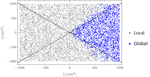
We found that for all points with $\mu_{2},\mu_{3}>0$, the chosen minimum remains the global one upon the addition of soft breaking terms. We also verify that it is the only global minimum of the resulting potential, not a degenerate global minimum. If $\mu_{2}$ or $\mu_{3}$ is significantly negative, the selected minimum unavoidably becomes local. However we also found many points where one of the two parameters, $\mu_{2}$ or $\mu_{3}$, is slightly negative, but the minimum remains global. Thus, requiring $\mu_{2},\mu_{3}>0$ is a sufficient but not necessary assumption for staying in the global minimum.

We illustrate this observation with the scatter plot in Fig. 1, where we start with the symmetric model with $\lambda_{2}=0.6$, $\lambda_{3}=-0.7$, select a minimum of type A, perform a four-parameter scan over soft breaking parameters, and project the results onto $(\Sigma,\delta)$ plane. We focus here on relatively small values of these two parameters. At the black lines, $\mu_{2}$ or $\mu_{3}$ changes sign. However the boundary between “always local” and “always global” parameter space regions does not coincide with the black lines and is in fact blurred. A very similar picture is observed for other parameters of the symmetric model.

What we gain from this exercise is the following insight: if one wants to build a softly broken $\Sigma(36)$ 3HDM with a vacuum at the brink of absolute tree-level stability, one should explore the parameter space regions along these lines.

Decoupling limit in multi-Higgs models refers to the regime in which additional, non-SM scalars are very heavy, so that we are left at the electroweak scale with the single Higgs particle whose tree-level properties approach the properties if the SM Higgs [33]. Decoupling limit is a weaker statement than the exact decoupling theorem, which requires all the effects induced by heavy non-standard particles to asymptotically disappear in the large mass limit. It is well known that, in the 2HDM and 3HDM, certain decays of the SM-like Higgs boson receive finite corrections from the charged Higgs boson loops even if their masses are very large [34, 35]. Thus, it is worth scrutinizing the properties of the SM-like Higgs boson in the decoupling limit.

In the 3HDM, we can also define in a similar manner the 2HDM-like limit, when two neutral and a pair of charged Higgses are heavy and decouple from the remaining relatively light 2HDM-like sector. Similarly to the distinction between the decoupling theorem and decoupling limit, decays of the scalars in this 2HDM-like sector may show deviations with respect to the 2HDM which would mimic the mass spectrum of the 3HDM with one generation of very heavy Higgses. This comparison would require a dedicated work.

Whether a multi-Higgs model can exhibit the SM decoupling limit depends on its symmetry content. The recent studies [36, 37, 38] proved that a symmetry-constrained multi-Higgs-doublet model allows for the decoupling limit only when the vev alignment preserves the symmetry group. In the 3HDMs with Higgs doublets in the 3D irreducible representation of the global symmetry group $G$, including the case of $\Sigma(36)$, the vev alignment unavoidably breaks the symmetry group, which makes the decoupling limit unattainable. This is also clearly seen by the single quadratic parameter $m^{2}$ in the $\Sigma(36)$-invariant 3HDM.

The presence of soft breaking terms lead to models without any exact symmetry and, therefore, can display the decoupling regime. If both $\mu_{2},\mu_{3}\gg|\lambda_{3}|v^{2}$, one can expand the neutral Higgs masses Eqs. (27)–(31) as

$$m^{2}_{h_{1},h_{2}}\approx\mu_{2}+|\lambda_{3}|v^{2}\mp\frac{x}{2}|\lambda_{3}|v^{2}\,,\quad m^{2}_{H_{1},H_{2}}\approx\mu_{3}+|\lambda_{3}|v^{2}\mp\frac{x}{2}|\lambda_{3}|v^{2}\,.$$

(35)

One observes the natural scale separation for the two heavy “multiplets”: the squared-masses of $H_{1}^{\pm}$, $h_{1}$ and $h_{2}$ stay at the scale $\mu_{2}$, while $H_{2}^{\pm}$, $H_{1}$ and $H_{2}$ reside at the scale $\mu_{3}$. Within each multiplet, one observes the same mass splitting pattern:

$$m_{H_{1}^{\pm}}^{2}-m_{h_{1}}^{2}=\frac{1}{2}v^{2}\left[\lambda_{2}+\lambda_{3}f(x)\right]\,,\quad m_{h_{2}}^{2}-m_{h_{1}}^{2}=x|\lambda_{3}|v^{2}\,,$$

(36)

with $f(x)=x+1$ for $\lambda_{3}>0$ (points $B$ and $C$) and $f(x)=2-x$ for $\lambda_{3}<0$ (points $A$ and $A^{\prime}$), and exactly the same splitting for $H_{2}^{\pm}$, $H_{1}$, $H_{2}$. Notice that since $0\leq x\leq 1$, the function $f(x)$ lies between 1 and 2 for any choice of the minimum.

Thus, we observe another structural feature of the softly broken model driven by the large symmetry of the parent model: in the SM-like decoupling limit, the decoupled sector has a rigid structure of its mass spectrum.

For the 2HDM-like decoupling limit, we assume that $\mu_{3}$ is large, while $\mu_{2}$ is of the same order of magnitude as $\lambda_{3}v^{2}$. The approximate results of Eq. (35) driven by large $|\delta|$ remain valid, but the mass scales of $h_{i}$ and $H_{i}$ are now different. The heavy scalars may be dynamically decoupled from the lighter degrees of freedom, but this does not mean their spectrum can be arbitrary. In fact, the heavy scalars display the same pattern of mass splitting shown in Eq. (36) as the lighter Higgses. Put simply, decoupling does not imply structural independence of the two sectors.

We also stress that the 2HDM-like model emerging after decoupling of the heavier scalars is not the general 2HDM but a rather constrained version of it. It closely resembles the 2HDM equipped with an approximate $\mathbb{Z}_{2}$ symmetry and further constrained by additional relations among parameters. Investigation of the phenomenological features of the resulting 2HDM-like model deserves a dedicated study.

In the parent $\Sigma(36)$ 3HDM, each of the possible minima is still invariant under a subgroup of $\Sigma(36)$. As a result, the scalar spectrum contains states stabilized against decay by these residual symmetries. In particular, tree-level trilinear couplings of such states to $h_{SM}$ pairs are all vanishing. However, the vev alignment preserving soft breaking terms, in general, remove all the symmetries from the model. As a result, the Higgses which were previously stabilized by residual symmetries are not protected anymore and can decay to the SM-like Higgses and further to the SM fields.

To understand how these decays proceed, suppose that $h_{1}$ is the lightest non-SM-like scalar. In the parent symmetric model, we had very few trilinear couplings involving $h_{1}$. With the soft breaking terms, one adds a few more terms, but the interaction vertices $h_{1}h_{SM}h_{SM}$ and $h_{1}h_{SM}h_{SM}h_{SM}$ which could generate tree-level decays of $h_{1}$ are still absent. Thus, there is no tree-level path to the decay of $h_{1}$.

Next, we checked scalar combinations which could lead to one-loop decays through the diagrams shown in Fig. 2. We found that there exist matching trilinear and quartic couplings ($h_{1}XY$ and $XYh_{SM}h_{SM}$ for topology 1, $h_{1}h_{SM}XY$ and $XYh_{SM}$ for topology 2) which share the same pairs of scalars $XY$. These matching pairs appear only with soft breaking terms; they were absent in the symmetric model.

These diagrams induce decay of $h_{1}$, which may be suppressed due to a number of reasons (loop factors, small couplings, subthreshold effects for $m_{h_{1}}<2m_{h_{SM}}$). If this suppression is significant, it may lead to displaced vertex signals which could be seen at colliders. Calculation of these decays should be an important part of a detailed phenomenological study of the softly broken $\Sigma(36)$ 3HDM.

References

- [1] G. C. Branco, P. M. Ferreira, L. Lavoura, M. N. Rebelo, M. Sher and J. P. Silva, Phys. Rept. 516, 1-102 (2012) [arXiv:1106.0034 [hep-ph]].
- [2] S. Kanemura, K. Tsumura, K. Yagyu and H. Yokoya, Phys. Rev. D 90, 075001 (2014) [arXiv:1406.3294 [hep-ph]].
- [3] I. P. Ivanov, Prog. Part. Nucl. Phys. 95, 160-208 (2017) [arXiv:1702.03776 [hep-ph]].
- [4] G. Arcadi, A. Djouadi and M. Raidal, Phys. Rept. 842, 1-180 (2020) [arXiv:1903.03616 [hep-ph]].
- [5] S. Weinberg, Phys. Rev. Lett. 37, 657 (1976).
- [6] M. Leurer, Y. Nir and N. Seiberg, Nucl. Phys. B 398, 319-342 (1993) [arXiv:hep-ph/9212278 [hep-ph]].
- [7] R. González Felipe, I. P. Ivanov, C. C. Nishi, H. Serôdio and J. P. Silva, Eur. Phys. J. C 74, no.7, 2953 (2014) [arXiv:1401.5807 [hep-ph]].
- [8] I. P. Ivanov and E. Vdovin, Eur. Phys. J. C 73, no.2, 2309 (2013) [arXiv:1210.6553 [hep-ph]].
- [9] N. Darvishi and A. Pilaftsis, Phys. Rev. D 101, no.9, 095008 (2020) [arXiv:1912.00887 [hep-ph]].
- [10] N. Darvishi, M. R. Masouminia and A. Pilaftsis, [arXiv:2106.03159 [hep-ph]].
- [11] C. C. Nishi, Phys. Rev. D 74, 036003 (2006) [erratum: Phys. Rev. D 76, 119901 (2007)] [arXiv:hep-ph/0605153 [hep-ph]].
- [12] I. de Medeiros Varzielas, S. F. King, C. Luhn and T. Neder, JHEP 11, 136 (2017) [arXiv:1706.07606 [hep-ph]].
- [13] I. P. Ivanov, C. C. Nishi, J. P. Silva and A. Trautner, Phys. Rev. D 99, no.1, 015039 (2019) [arXiv:1810.13396 [hep-ph]].
- [14] I. P. Ivanov, C. C. Nishi and A. Trautner, Eur. Phys. J. C 79, no.4, 315 (2019) [arXiv:1901.11472 [hep-ph]].
- [15] I. de Medeiros Varzielas and I. P. Ivanov, Phys. Rev. D 100, no.1, 015008 (2019) [arXiv:1903.11110 [hep-ph]].
- [16] I. P. Ivanov and C. C. Nishi, JHEP 01, 021 (2015) [arXiv:1410.6139 [hep-ph]].
- [17] I. de Medeiros Varzielas, S. F. King, C. Luhn and T. Neder, Phys. Lett. B 775, 303-310 (2017) [arXiv:1704.06322 [hep-ph]].
- [18] G. Segre and H. A. Weldon, Phys. Lett. B 83, 351-354 (1979).
- [19] W. Grimus and P. O. Ludl, J. Phys. A 43, 445209 (2010) [arXiv:1006.0098 [hep-ph]].
- [20] A. Merle and R. Zwicky, JHEP 02, 128 (2012) [arXiv:1110.4891 [hep-ph]].
- [21] C. Hagedorn, A. Meroni and L. Vitale, J. Phys. A 47, 055201 (2014) [arXiv:1307.5308 [hep-ph]].
- [22] S. J. Rong, Phys. Rev. D 95, no.7, 076014 (2017) [arXiv:1604.08482 [hep-ph]].
- [23] I. P. Ivanov, V. Keus and E. Vdovin, J. Phys. A 45, 215201 (2012) [arXiv:1112.1660 [math-ph]].
- [24] G. C. Branco, J. M. Gerard and W. Grimus, Phys. Lett. B 136, 383-386 (1984).
- [25] I. de Medeiros Varzielas and D. Emmanuel-Costa, Phys. Rev. D 84, 117901 (2011) [arXiv:1106.5477 [hep-ph]].
- [26] I. de Medeiros Varzielas, D. Emmanuel-Costa and P. Leser, Phys. Lett. B 716, 193-196 (2012) [arXiv:1204.3633 [hep-ph]].
- [27] I. P. Ivanov and L. Lavoura, Eur. Phys. J. C 73, no.4, 2416 (2013) [arXiv:1302.3656 [hep-ph]].
- [28] G. Bhattacharyya, I. de Medeiros Varzielas and P. Leser, Phys. Rev. Lett. 109, 241603 (2012) [arXiv:1210.0545 [hep-ph]].
- [29] I. de Medeiros Varzielas and D. Pidt, J. Phys. G 41, 025004 (2014) [arXiv:1307.0711 [hep-ph]].
- [30] I. de Medeiros Varzielas and D. Pidt, JHEP 11, 206 (2013) [arXiv:1307.6545 [hep-ph]].
- [31] M. Fallbacher and A. Trautner, Nucl. Phys. B 894, 136-160 (2015) [arXiv:1502.01829 [hep-ph]].
- [32] P. M. Ferreira, I. P. Ivanov, E. Jiménez, R. Pasechnik and H. Serôdio, JHEP 01, 065 (2018) [arXiv:1711.02042 [hep-ph]].
- [33] J. F. Gunion and H. E. Haber, Phys. Rev. D 67, 075019 (2003) [arXiv:hep-ph/0207010 [hep-ph]].
- [34] A. Arhrib, M. Capdequi Peyranere, W. Hollik and S. Penaranda, Phys. Lett. B 579, 361-370 (2004) [arXiv:hep-ph/0307391 [hep-ph]].
- [35] G. Bhattacharyya and D. Das, Phys. Rev. D 91, 015005 (2015) [arXiv:1408.6133 [hep-ph]].
- [36] M. Nebot, Phys. Rev. D 102, no.11, 115002 (2020) [arXiv:1911.02266 [hep-ph]].
- [37] F. Faro, J. C. Romao and J. P. Silva, Eur. Phys. J. C 80, no.7, 635 (2020) [arXiv:2002.10518 [hep-ph]].
- [38] S. Carrolo, J. C. Romão, J. P. Silva and F. Vazão, Phys. Rev. D 103, no.7, 075026 (2021) [arXiv:2102.11303 [hep-ph]].