The Fourier formalism for relativistic axion-photon conversion,
with astrophysical applications

Determining the elementary particle content beyond the established Standard Model is a central goal of contemporary high-energy physics. The QCD axion (cf. Wilczek 1978) and axion-like particles (axions) comprise a well-motivated class of hypothetical particles that frequently appear in extensions of the Standard Model, including effective theories derived from string theory Svrcek and Witten 2006. Both the QCD axion and axions can be understood as pseudo-Nambu-Goldstone bosons of broken, approximate symmetries, and the QCD axion provides the leading candidate solution to the strong CP-problem. In this paper we will simply use ‘axions’ to refer to the QCD axion and axion-like particles, as our results apply equally to these particles.

Axions can naturally be very light, with feeble couplings to matter and radiation, and provide an increasingly popular candidate for explaining the nature of dark matter Preskill et al. 1983; Abbott and Sikivie 1983; Dine and Fischler 1983. Characteristic of axions is their coupling to electromagnetism through the Lagrangian term

$${\cal L}_{\rm int}=\frac{1}{4}g_{a\gamma}aF_{\mu\nu}\tilde{F}^{\mu\nu}$$

where $g_{a\gamma}$ denotes the axion-photon coupling and the axion, $a$, is assumed to have a mass $m_{a}$. This term induces a mixing between the photon and the axion in backgrounds with non-vanishing electromagnetic fields, opening the possibility to interconvert axions and photons. Such interconversion underpins the majority of the experimental and observational efforts to search for axions (cf. Raffelt 1996; Group 2020; Irastorza and Redondo 2018; Asztalos et al. 2004; Lawson et al. 2019). Particularly powerful are searches for axion-induced distortions in the spectra of luminous X-ray and gamma-ray sources located in galaxy clusters Hooper and Serpico 2007; Chelouche et al. 2009; Wouters and Brun 2013; Conlon and Marsh 2013; Berg et al. 2017; Marsh et al. 2017; Chen and Conlon 2018; Conlon et al. 2017; Reynolds et al. 2019; Abramowski et al. 2013; Cicoli et al. 2014; Meyer et al. 2014; Meyer and Conrad 2014; Ajello et al. 2016a; Zhang et al. 2018; Malyshev et al. 2018; Xia et al. 2018; Galanti et al. 2019; Majumdar et al. 2018; Liang et al. 2019; Bu and Li 2019; Li et al. 2021; Guo et al. 2021; Cheng et al. 2020; Carenza et al. 2021; Reynés et al. 2021. State-of-the-art analyses using high-quality data from the Chandra X-ray observatory have bounded axion-induced spectral distortions from the AGN at the centre of the Perseus cluster to the few percent level, leading to some of the strongest limits on the axion-photon coupling to date ($g_{a\gamma}\leq 7.9\times 10^{-13}~{\rm GeV}^{-1}$ for $m_{a}<10^{-12}~{\rm eV}$ Reynolds et al. 2019).

The observational prospects are very good for even more sensitive searches for axions using existing and planned X-ray and gamma-ray telescopes, such as Athena Nandra et al. 2013 and the Cerenkov Telescope Array Acharya et al. 2018. However, such studies will be limited by modelling uncertainties affecting the axion-photon mixing. The conversion probability is in general a complicated function of the mode energy, the axion parameters $m_{a}$ and $g_{a\gamma}$, as well as the plasma density and magnetic field along the particle trajectory. The robustness of the predictions to astrophysical modelling uncertainties has been investigated by several groups over the past decade Angus et al. 2014; Meyer et al. 2014; Galanti and Roncadelli 2018; Libanov and Troitsky 2020; Bu and Li 2019, typically finding that limits on $g_{a\gamma}$ can change by a factor of a few depending on the magnetic field model employed. A recent, unusual contribution to these studies is reference Libanov and Troitsky 2020, which investigated the robustness of certain gamma-ray constraints assuming — as a limiting but ostensibly observationally consistent case — that the cluster magnetic field in Perseus is highly regular, finding much weaker limits than those of Ajello et al. 2016a.¹¹ 1 We reexamine the astrophysical viability of this model in section VII. Common to all these studies is the reliance on very simple magnetic field models to generate physical intuition (typically, a constant magnetic field), and numerical simulations to examine more involved models. This has left room for some confusion as to what properties of the magnetic field really drive the appearance of features in the conversion probability, and how robust the predictions really are.

In this paper, we revisit the theory of axion-photon conversion, and develop a powerful new method calculating and interpreting axion-photon mixing. Our results are equally valid for applications in the laboratory and space, but our main focus is on astrophysical applications involving conversion of high-energy photons into relativistic axions. Our approach is inspired by — and will be particularly useful for — the emerging sub-field of precision X-ray searches for axions Conlon and Marsh 2013; Berg et al. 2017; Marsh et al. 2017; Chen and Conlon 2018; Conlon et al. 2017; Reynolds et al. 2019; Reynés et al. 2021, which presently constrain the mixing probability to be no larger than a few percent. For such weak mixing, the system is in the perturbative regime, and the goal of this paper is to demonstrate the significant conceptual, calculational and methodological advances that can be gained using perturbation theory.

It is well-known that the classical, linearised axion-photon system can be written as a Schrödinger-like equation, with time replaced by the spatial coordinate, say $z$, along the direction of propagation Raffelt and Stodolsky 1988. In quantum mechanics, the asymptotic, perturbative transition amplitude can be expressed as a Fourier transform of the interaction Hamiltonian. In this paper, we show that a similar, but more subtle, statement also holds for classical axion-photon mixing.

In the simplest case, which is directly relevant for gamma-ray searches, the mass of the axion is always larger than the plasma frequency. We find that, to leading order in $g_{a\gamma}$, the axion-photon transition amplitude involving such massive axions is given by a sum of Fourier cosine and sine transforms of the (relevant component of the) magnetic field, $B$. The conversion probability is then given by the power spectrum of $B$. We derive a version of the Wiener–Khintchine theorem that shows that the conversion probability is equal to the Fourier cosine transform of the magnetic autocorrelation function. Strikingly, this means that questions about the spectrum of oscillations induced by axion-photon conversion map directly onto questions about the real-space properties of the magnetic autocorrelation. This constructively answers the questions of what properties of the magnetic field are reflected in the conversion probability. We demonstrate how to apply this formalism in a series of examples, ranging from the simple to the general. In particular, we analytically calculate the conversion probability and the magnetic autocorrelation function for a magnetic field expressed as a Fourier series. Since any physically relevant magnetic field can be expressed in such a way, this explicitly solves the problem of weak axion-photon mixing, for sufficiently massive axions.

Somewhat more subtle is the case of massless axions. In this case, the transition amplitude is no longer given by a Fourier transform obtained by integrating over the spatial coordinate $z$, as in the massive case. However, the amplitude can be written as a Fourier transform obtained by integrating over the variable

$$\varphi(z)=\frac{1}{2}\int_{0}^{z}dz^{\prime}\,\omega_{\rm pl}^{2}(z^{\prime})\,.$$

Again we find that the transition amplitude is given by cosine and sine transforms, but this time of the function $G=B/\omega_{\rm pl}^{2}$. The conversion probability is given by the power spectrum of $G$, or equivalently by our version of the Wiener–Khintchine theorem, as the cosine transform of the autocorrelation function of $G$ (in $\varphi$-space).

In general, there may be some regions where $m_{a}<\omega_{\rm pl}$, and others where $m_{a}>\omega_{\rm pl}$. In this case, it is not possible to express the transition amplitude as a single Fourier transform. However, we find that the transition amplitude reduces to a sum of ‘non-resonant’ contributions that are given by Fourier transforms of $G$ (one for each region where $m_{a}-\omega_{\rm pl}$ has a definite sign), and a sum of ‘resonant’ contributions (from points where $m_{a}=\omega_{\rm pl}$).

An often used method to analytically evaluate resonant axion-photon mixing is the stationary phase approximation. We show that, in the relativistic limit, the resonant amplitude calculated from the stationary phase approximation is enhanced by a factor of $\omega/m_{a}$, which is very large for light axions emerging from X-rays or gamma rays. However, we also show that a naive application of the stationary phase approximation to the resonant conversion gives a result that is highly inaccurate. We address this issue by deriving a modified form of the stationary phase approximation that is relevant for relativistic axion-photon conversion: with this new formula, we see that in careful calculations of the amplitude, the non-resonant contributions are generically at least as large as the resonant contributions.

Fast Fourier Transforms (FFTs), and related methods, have revolutionised digital signal processing by providing highly effective ways to numerically evaluate the discrete Fourier transform. We show that with our formalism, axion-photon conversion can be evaluated using methods based on FFTs. This drastically reduces the computational effort in determining the effects of axion-photon mixing, and allows for effective marginalisation or Monte Carlo over astrophysical magnetic fields and plasma densities. See also Conlon and Rummel 2019 for a discussion of FFT techniques applied to axion searches.

Since magnetic auto-correlations determine the predictions of perturbative axion-photon conversion, it is important to re-examine what is known about astrophysical magnetic fields in the environments most promising for axion searches. To this end, we discuss the expected properties of magnetic fields in galaxy clusters. We review the arguments for turbulence in the intracluster medium (ICM), and the classes of models used in astrophysical axion searches. In particular, we critically examine the recently proposed ‘regular model’ of Libanov and Troitsky 2020, finding it at odds with observations.

We suggest that future studies of the magnetic field autocorrelation function in state-of-the-art magnetohydrodynamic simulations of the ICM will be very useful in improving the sensitivity of axion searches. Moreover, our formalism could lead to new methodologies for axion searches, e.g. by generating the relevant mixing probabilities directly from an observationally inferred class of autocorrelation functions, without ever explicitly solving the Schrödinger equation.

This paper is organised as follows: in section II we review the classical theory of axion-photon conversion, and how it can be understood through non-relativistic quantum mechanics. We analytically develop the new formalism in sections III–V, for the cases of a comparatively heavy axion (section III), a very light axion (section IV), and the intermediate, general case (section V). We then test relevant aspects numerically in section VI, and discuss numerical implementations using discrete, Fourier-like transforms. In section VII, we discuss what is known about magnetic autocorrelations in the relevant astrophysical environments, and we indicate new possible directions for the methodology of axion searches. We conclude in section VIII.

The most important new results of this paper are (in no particular order) i) the relation between the non-resonant conversion probability and the magnetic autocorrelation function given by equations (30), (79) and (115); ii) accounting carefully for both resonant and non-resonant contributions when $\omega_{\rm pl}=m_{a}$ at one or more points along the trajectory, cf. section V.2; iii) the demonstration that one can use highly efficient FFT methods to calculate the conversion probabilities, cf. section VI.2; iv) the identification of new, promising methods that are made possible by the new formalism, and which can open up new directions for axion searches, cf. section VII.3.

In this section, we begin by reviewing the axion-photon mixing in magnetic fields following  Raffelt and Stodolsky 1988; Battye et al. 2020. This leads to a Schrödinger-like equation from which the transition amplitudes can be calculated order-by-order in perturbation theory Raffelt and Stodolsky 1988, in direct analogy with time-dependent perturbation theory in quantum mechanics. The axion-photon interaction is described by the following Lagrangian

$$\mathcal{L}=-\frac{1}{4}F^{\mu\nu}F_{\mu\nu}+\frac{1}{2}\left(\partial_{\mu}\,a\partial^{\mu}a-m_{a}^{2}a^{2}\right)-\frac{g_{a\gamma}}{4}a\,F_{\mu\nu}\tilde{F}^{\mu\nu}\,,$$

(1)

where $a$ is the axion field, $A_{\mu}$ is the photon field, $F_{\mu\nu}$ is the electromagnetic tensor, $\tilde{F}_{\mu\nu}=\tfrac{1}{2}\epsilon_{\mu\nu\lambda\rho}F^{\lambda\rho}$. We have neglected the effects of Faraday rotations and QED birefringence at low energy.²² 2 The Faraday effect is inversely proportional to the energy, and completely negligible at X-ray energies or higher. Moreover, at X-ray energies, the QED birefringence contribution would in a typical galaxy cluster environments with $\mu{\rm G}$ magnetic fields and plasma frequencies of the order of $\omega_{\rm pl}\sim 10^{-12}$ eV lead to a fractional correction to $\Delta_{\gamma}$, that we define in (8), of order $10^{-16}$. The QED contribution scales like $E^{2}B^{2}$, and is less suppressed, and sometimes even non-negligible, in environments with strong magnetic fields probed at very high energies (cf. Davies et al. 2021 for a recent example). This equation of motion are the Klein-Gordon equation for the axion field, and an extension of Maxwell’s equations. The linearised equations around a static background magnetic field ${\bf B}_{0}$ are given by

$$\begin{split}(\Box+m_{a}^{2})a&=-g_{a\gamma}\dot{\bf A}\cdot{\bf B}_{0}\,,\\ (\Box+\omega_{\rm pl}^{2}){\bf A}&=g_{a\gamma}\dot{a}\,{\bf B}_{0}\,,\end{split}$$

(2)

where we included the plasma frequency $\omega_{\rm pl}$. Most works on axion-photon mixing (from Raffelt and Stodolsky 1988 to the more recent X-ray and gamma-ray studies, see e.g. Horns et al. 2012) further simplify this system by assuming that all background quantities only vary along the $z$-direction, which is taken to be the axion or photon propagation direction.³³ 3 For a recent discussions of extensions to anisotropic plasmas, see Battye et al. 2020; Millar et al. 2021. We consider a right-moving plane wave in the $z$-direction, and write the components of the background magnetic field respectively as $B_{x}$ and $B_{y}$. Equations (2) now become

$$\begin{split}(\omega^{2}+\partial_{z}^{2}-m_{a}^{2})a&=i\omega g_{a\gamma}(A_{x}B_{x}+A_{y}B_{y})\,,\\ (\omega^{2}+\partial_{z}^{2}-\omega_{\rm pl}^{2})A_{j}&=-i\omega g_{a\gamma}aB_{j}\quad j=x,y\,.\end{split}$$

(3)

In the relativistic limit, the equations of motion can be reduced to first order by appealing to the rotating wave approximation: $\omega^{2}+\partial_{z}^{2}=(\omega+i\partial_{z})(\omega-i\partial_{z})\simeq 2\omega(\omega-i\partial_{z})$.⁴⁴ 4 An alternative method to arrive at the first-order equations is to use the WKB approximation, which is applicable also in the non-relativistic case Battye et al. 2020. After a shift of the axion field $a\rightarrow-ia$, the equations of motion are

$$\begin{split}(\omega-i\partial_{z})a&=\frac{m_{a}^{2}}{2\omega}a-\frac{g_{a\gamma}}{2}(A_{x}B_{x}+A_{y}B_{y})\,,\\ (\omega-i\partial_{z})A_{j}&=\frac{\omega_{\rm pl}^{2}}{2\omega}A_{j}-\frac{g_{a\gamma}B_{j}}{2}a\quad j=x,y\,.\end{split}$$

(4)

These classical mixing equations are now of the form of the Schrödinger equation, with time replaced by the spatial coordinate $z$ Raffelt and Stodolsky 1988:

$$i\frac{d}{dz}\Psi(z)=(H_{0}+H_{I})\Psi(z)\,.$$

(5)

Here the axion field and the components of the vector potential are components of the ‘Schrödinger-picture state vector’

$$\Psi(z)=\begin{pmatrix}A_{x}\\ A_{y}\\ a\end{pmatrix}\,,$$

(6)

where we have suppressed the dependence on the mode energy $\omega$. The basis vectors are assumed to be $z$-independent, but the coefficients of the state vector evolve with $z$. The Hamiltonian is decomposed into free and interaction parts

$$H_{0}=\omega\mathbb{I}+\begin{pmatrix}\Delta_{\gamma}&0&0\\ 0&\Delta_{\gamma}&0\\ 0&0&\Delta_{a}\end{pmatrix}\quad H_{I}=\begin{pmatrix}0&0&\Delta_{x}\\ 0&0&\Delta_{y}\\ \Delta_{x}&\Delta_{y}&0\end{pmatrix}\,,$$

(7)

and

$$\begin{split}\Delta_{a}&=-\frac{m_{a}^{2}}{2\omega}\,,\\ \Delta_{\gamma}&=-\frac{\omega_{\rm pl}^{2}}{2\omega}\,,\\ \Delta_{j}&=\frac{g_{a\gamma}B_{j}}{2}\quad\,.\\ \end{split}$$

(8)

where $j=x,y$.⁵⁵ 5 In the non-relativistic version of these identities, the factors of $\omega$ are replaced by the norm of the wavevector, which in general depends on $z$. The formal solution to the Schrödinger-like equation is

$$\Psi(z)=U(z,0)\Psi(0)$$

where

$$U(z,0)={\cal P}_{z}e^{i\int_{0}^{z}dz^{\prime}\,(H_{0}+H_{I})}\,,$$

(9)

and where ${\cal P}_{z}$ denotes the path-ordering operator. The $z$-evolution operator $U(z,0)$ is implicitly energy dependent. Numerical solutions can be found by discretising the $z$-direction into a sufficiently large number of ‘cells’ so that the Hamiltonian is approximately constant in each cell, and the total evolution operator $U$ is the product of the evolution operators for all cells, appropriately ordered. Such a numerical approach is very common in astrophysical searches for axions, but becomes computationally costly when the mixing occurs over large distances with non-trivially varying magnetic fields, when the energy resolution needs to be finely sampled, and when a large number of possible magnetic field configurations must be considered.

However, the structure of equation (5) is suggestive of different approach: perturbation theory in direct analogy with time-dependent perturbation theory in quantum mechanics. This is most conveniently studied in the interaction picture, where the equations of motion are given by

$$i\frac{d}{dz}\Psi_{\rm int}=H_{\rm int}\Psi_{\rm int}\,,$$

(10)

where $H_{\rm int}=U_{0}^{\dagger}H_{I}U_{0}$ and $\Psi_{\rm int}=U_{0}^{\dagger}\Psi$ with the zeroth-order evolution operator $U_{0}={\rm exp}\left(-i\int_{0}^{z}dz^{\prime}\,H_{0}\right)$. The general solution can be expressed as an expansion in the interaction Hamiltonian,

		$\displaystyle\Psi_{\rm int}(z)=$		(11)
		$\displaystyle\sum_{n=0}^{\infty}\left(-i\right)^{n}\int_{0}^{z}dz_{1}^{\prime}\ldots\int_{0}^{z_{n-1}}dz_{n}^{\prime}\,H_{\rm int}(z_{1}^{\prime})\ldots H_{\rm int}(z_{n}^{\prime})\,\Psi_{\rm int}(0),$

which equivalently corresponds to an expansion in the coupling constant, $g_{a\gamma}$. To linear order in perturbation theory, the state in the interaction picture is given by

$$\Psi_{\rm int}(z)=\Psi_{\rm int}(0)-i\int_{0}^{z}dz^{\prime}\,H_{\rm int}\Psi_{\rm int}(0)\,.$$

(12)

In the original Schrödinger-picture basis, this corresponds to

$$\Psi(z)=\Big(U_{0}(z,0)+\int_{0}^{z}dz^{\prime}\,U_{0}(z,z^{\prime})H_{I}(z^{\prime})U_{0}(z^{\prime},0)\Big)\Psi(0)\,.$$

(13)

The perturbative expansion can be expressed using Feynman diagrams, where each order in $H_{I}$ corresponds to an additional axion-photon mixing vertex, and where the zeroth-order evolution operator $U_{0}$ propagates the state between the vertices.

We are interested in the transition amplitude of an initial photon state emerging as an axion. This corresponds to the initial condition $\Psi(0)=(1,0,0)^{\rm T}$ if the photon is linearly $x$-polarised, and $\Psi(0)=(0,1,0)^{\rm T}$ if its $y$-polarised. With $j=x,y$ the leading order (LO) transition amplitude is then given by Raffelt and Stodolsky 1988

$$\begin{split}\mathcal{A}_{\gamma_{j}\rightarrow a}&=(0,0,1)\cdot\Psi(z)=-i\int_{0}^{z}dz^{\prime}\,\Delta_{j}(z^{\prime})\,e^{i\int_{0}^{z^{\prime}}dz^{\prime\prime}\,(\Delta_{a}-\Delta_{\gamma})}\,.\end{split}$$

(14)

The conversion probability is obtained by squaring this transition amplitude: $P_{\gamma_{j}\rightarrow a}=|\mathcal{A}_{\gamma_{j}\rightarrow a}|^{2}$. This conversion probability calculated from the (classical) Schrödinger-like equation gives the ratio of the squared axion field to the squared electric field, which also corresponds to the observationally relevant flux ratio of axion and photons.

Next-to-leading-order (NLO) corrections appear at order ${\cal O}(g_{a\gamma}^{3})$ in the amplitude from the 3-vertex Feynman diagram: ‘photon $\to$ axion $\to$ photon $\to$ axion´. The LO conversion probability appear at ${\cal O}(g_{a\gamma}^{2})$, with higher-order corrections appearing at ${\cal O}(g_{a\gamma}^{4})$. Thus, the perturbative expansion is generically a good approximation when the conversion probability is small, with fractional corrections at the same order as the conversion probability (i.e. a 1% perturbative conversion probability generically receives corrections at the order of $0.01\%$, cf. section VI.4 for a detailed discussion).

The above equations lead to unitary time evolution, and so neglects possible photon absorption. This is a good approximation when the medium is optically thin over the region at which axion-photon mixing occurs, which is the case for many astrophysical applications of practical relevance, cf. e.g. Marsh et al. 2017. However, including photon absorption is straightforward and leads to a modified Schrödinger-like equation that features a non-Hermitian Hamiltonian:

$$i\frac{d}{dz}\Psi(z)=(H_{0}+H_{I}-iD)\Psi(z)\,,$$

where

$$D(z)=\begin{pmatrix}\beta(z)&0&0\\ 0&\beta(z)&0\\ 0&0&0\end{pmatrix}$$

encodes the damping. The the real function $\beta$ depends on the absorption cross-section and astrophysical parameters, such as the free electron density. Since $[D(z),H_{0}(z^{\prime})]=0$, it is straightforward to include damping as a zeroth-order modification to the perturbative expansion: equation (10) in the interaction picture still holds, but with the unitary operator $U_{0}$ now replaced by the non-unitary transfer matrix

$$T_{0}(z_{2},z_{1})=e^{-i\int_{z_{1}}^{z_{2}}dz^{\prime}\big(H_{0}-iD\big)}\,,$$

so that $\Psi_{\rm int}(z)=T_{0}^{-1}(z,0)\Psi(0)$ and $H_{\rm int}=T_{0}^{-1}H_{I}T_{0}$. This way, photon absorption modifies the zeroth-order propagator, and to linear order the Schrödinger-picture state is given by:

$$\Psi(z)=\Big(T_{0}(z,0)+\int_{0}^{z}dz^{\prime}\,T_{0}(z,z^{\prime})H_{I}(z^{\prime})T_{0}(z^{\prime},0)\Big)\Psi(0)\,.$$

(15)

In the following, we will neglect photon absorption.

In this paper, we will almost exclusively focus on polarised transition probabilities, involving a single component of the magnetic field. However, many bright astrophysical sources that are suitable for searches for axions are unpolarised. The conversion probability for an upolarised source of photons is $P_{\gamma\to a}=\frac{1}{2}\left(P_{\gamma_{x}\to a}+P_{\gamma_{y}\to a}\right)$, and the survival fraction of the unpolarised flux is

$$P_{\gamma\to\gamma}=1-P_{\gamma\to a}=1-\frac{1}{2}\left(P_{\gamma_{x}\to a}+P_{\gamma_{y}\to a}\right)\,.$$

(16)

In the following, we will primarily consider the conversion probability for a linearly polarised photon (with respect to a fixed, Cartesian coordinate system), with the understanding that the unpolarised probability can easily be obtained using formula (16). For a discussion on polarised signals from axion-photon conversion, see Day and Krippendorf 2018.

Finally, and for context, we note that solving the Schrödinger-like equation for axion photon mixing is equivalent to solving the von Neumann equation for the corresponding density matrix, $\rho$, as is done in much of the literature. The equation of motion of $\rho$ is,

$$i\frac{d\rho}{dz}=[H_{0}+H_{I},\rho]\,,$$

and the diagonal elements of $\rho$ are interpreted as the square of the wavefunctions of the two photon polarisation and the axion, respectively. The time-evolution of the density matrix is given by

$$\rho(z)=U(z,0)\rho(0)U^{\dagger}(z,0)\,,$$

for the evolution operator of equation (9). Numerical solutions in this formalism proceed equivalently to the Schrödinger equation (i.e. by finding the $z$-evolution operator), and there is no significant conceptual or calculational difference between the two formalisms. In particular, photon absorption is accounted for in an identical manner in the two formalisms, by replacing the unitary evolution operator by a non-unitary transfer matrix, and the perturbative expansion of $U$ can be applies equally to the two formalisms. For this reason, we will not discuss the density-matrix formulation of this problem any further in this paper.

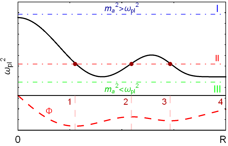
To leading order in the mixing, the amplitude for an initial photon state, linearly polarised along the $x$-direction, to transition into an axion is given by

$${\cal A}_{\gamma_{x}\to a}=-i\int_{0}^{z}dz^{\prime}\Delta_{x}(z^{\prime})e^{-i\Phi(z^{\prime})}\,,$$

(17)

where the phase is given by

$$\Phi(z^{\prime})=\int_{0}^{z^{\prime}}dz^{\prime\prime}\big[\Delta_{\gamma}(z^{\prime\prime})-\Delta_{a}\big]\,,$$

(18)

with $\Delta_{\gamma}$ and $\Delta_{a}$ as in equation (8). The phase $\Phi$ may both increase and decrease along the trajectory depending on the relative sizes of $\Delta_{\gamma}(z^{\prime})$ and $\Delta_{a}$. The key property of $\Phi$ that we use in this paper is that it can, in general, be factorised into a generalised spatial integration variable of equation (17) (say $z^{\prime}$ in the simplest case) multiplied by an independent, ‘conjugate’ parameter (say $1/\omega$). In this section, we focus on the simplest case when $\Delta_{\gamma}$ can be neglected, and the links to Fourier analysis are most apparent. We note that this factorisation is more subtle in the case of non-relativistic axions, which obey a similar Schrödinger-like equation but for which the factors of $1/\omega$ in (8) should be replaced by the inverse of a spatial wave-vector Battye et al. 2020, which depends on the spatial coordinate. In this paper, we focus on the simpler relativistic case.

References

- Wilczek (1978) F. Wilczek, Phys. Rev. Lett. 40, 279 (1978).
- Svrcek and Witten (2006) P. Svrcek and E. Witten, JHEP 06, 051 (2006), arXiv:hep-th/0605206 .
- Preskill et al. (1983) J. Preskill, M. B. Wise, and F. Wilczek, Phys. Lett. B 120, 127 (1983).
- Abbott and Sikivie (1983) L. F. Abbott and P. Sikivie, Phys. Lett. B 120, 133 (1983).
- Dine and Fischler (1983) M. Dine and W. Fischler, Phys. Lett. B 120, 137 (1983).
- Raffelt (1996) G. G. Raffelt, Stars as laboratories for fundamental physics: The astrophysics of neutrinos, axions, and other weakly interacting particles (1996).
- Group (2020) P. D. Group, Progress of Theoretical and Experimental Physics 2020 (2020), 10.1093/ptep/ptaa104, 083C01, https://academic.oup.com/ptep/article-pdf/2020/8/083C01/34673722/ptaa104.pdf .
- Irastorza and Redondo (2018) I. G. Irastorza and J. Redondo, Prog. Part. Nucl. Phys. 102, 89 (2018), arXiv:1801.08127 [hep-ph] .
- Asztalos et al. (2004) S. J. Asztalos et al. (ADMX), Phys. Rev. D 69, 011101 (2004), arXiv:astro-ph/0310042 .
- Lawson et al. (2019) M. Lawson, A. J. Millar, M. Pancaldi, E. Vitagliano, and F. Wilczek, Phys. Rev. Lett. 123, 141802 (2019), arXiv:1904.11872 [hep-ph] .
- Hooper and Serpico (2007) D. Hooper and P. D. Serpico, Phys. Rev. Lett. 99, 231102 (2007), arXiv:0706.3203 [hep-ph] .
- Chelouche et al. (2009) D. Chelouche, R. Rabadan, S. Pavlov, and F. Castejon, Astrophys. J. Suppl. 180, 1 (2009), arXiv:0806.0411 [astro-ph] .
- Wouters and Brun (2013) D. Wouters and P. Brun, Astrophys. J. 772, 44 (2013), arXiv:1304.0989 [astro-ph.HE] .
- Conlon and Marsh (2013) J. P. Conlon and M. C. D. Marsh, Phys. Rev. Lett. 111, 151301 (2013), arXiv:1305.3603 [astro-ph.CO] .
- Berg et al. (2017) M. Berg, J. P. Conlon, F. Day, N. Jennings, S. Krippendorf, A. J. Powell, and M. Rummel, Astrophys. J. 847, 101 (2017), arXiv:1605.01043 [astro-ph.HE] .
- Marsh et al. (2017) M. D. Marsh, H. R. Russell, A. C. Fabian, B. P. McNamara, P. Nulsen, and C. S. Reynolds, JCAP 12, 036 (2017), arXiv:1703.07354 [hep-ph] .
- Chen and Conlon (2018) L. Chen and J. P. Conlon, Mon. Not. Roy. Astron. Soc. 479, 2243 (2018), arXiv:1712.08313 [astro-ph.HE] .
- Conlon et al. (2017) J. P. Conlon, F. Day, N. Jennings, S. Krippendorf, and M. Rummel, JCAP 07, 005 (2017), arXiv:1704.05256 [astro-ph.HE] .
- Reynolds et al. (2019) C. S. Reynolds, M. D. Marsh, H. R. Russell, A. C. Fabian, R. Smith, F. Tombesi, and S. Veilleux, (2019), 10.3847/1538-4357/ab6a0c, arXiv:1907.05475 [hep-ph] .
- Abramowski et al. (2013) A. Abramowski et al. (H.E.S.S.), Phys. Rev. D 88, 102003 (2013), arXiv:1311.3148 [astro-ph.HE] .
- Cicoli et al. (2014) M. Cicoli, J. P. Conlon, M. C. D. Marsh, and M. Rummel, Phys. Rev. D 90, 023540 (2014), arXiv:1403.2370 [hep-ph] .
- Meyer et al. (2014) M. Meyer, D. Montanino, and J. Conrad, JCAP 09, 003 (2014), arXiv:1406.5972 [astro-ph.HE] .
- Meyer and Conrad (2014) M. Meyer and J. Conrad, JCAP 12, 016 (2014), arXiv:1410.1556 [astro-ph.HE] .
- Ajello et al. (2016a) M. Ajello et al. (Fermi-LAT), Phys. Rev. Lett. 116, 161101 (2016a), arXiv:1603.06978 [astro-ph.HE] .
- Zhang et al. (2018) C. Zhang, Y.-F. Liang, S. Li, N.-H. Liao, L. Feng, Q. Yuan, Y.-Z. Fan, and Z.-Z. Ren, Phys. Rev. D 97, 063009 (2018), arXiv:1802.08420 [hep-ph] .
- Malyshev et al. (2018) D. Malyshev, A. Neronov, D. Semikoz, A. Santangelo, and J. Jochum, (2018), arXiv:1805.04388 [astro-ph.HE] .
- Xia et al. (2018) Z.-Q. Xia, C. Zhang, Y.-F. Liang, L. Feng, Q. Yuan, Y.-Z. Fan, and J. Wu, Phys. Rev. D 97, 063003 (2018), arXiv:1801.01646 [astro-ph.HE] .
- Galanti et al. (2019) G. Galanti, F. Tavecchio, M. Roncadelli, and C. Evoli, Mon. Not. Roy. Astron. Soc. 487, 123 (2019), arXiv:1811.03548 [astro-ph.HE] .
- Majumdar et al. (2018) J. Majumdar, F. Calore, and D. Horns, JCAP 04, 048 (2018), arXiv:1801.08813 [hep-ph] .
- Liang et al. (2019) Y.-F. Liang, C. Zhang, Z.-Q. Xia, L. Feng, Q. Yuan, and Y.-Z. Fan, JCAP 06, 042 (2019), arXiv:1804.07186 [hep-ph] .
- Bu and Li (2019) J. Bu and Y.-P. Li, (2019), 10.1088/1674-4527/19/10/154, arXiv:1906.00357 [astro-ph.HE] .
- Li et al. (2021) H.-J. Li, J.-G. Guo, X.-J. Bi, S.-J. Lin, and P.-F. Yin, Phys. Rev. D 103, 083003 (2021), arXiv:2008.09464 [astro-ph.HE] .
- Guo et al. (2021) J. Guo, H.-J. Li, X.-J. Bi, S.-J. Lin, and P.-F. Yin, Chin. Phys. C 45, 025105 (2021), arXiv:2002.07571 [astro-ph.HE] .
- Cheng et al. (2020) J.-G. Cheng, Y.-J. He, Y.-F. Liang, R.-J. Lu, and E.-W. Liang, (2020), arXiv:2010.12396 [astro-ph.HE] .
- Carenza et al. (2021) P. Carenza, C. Evoli, M. Giannotti, A. Mirizzi, and D. Montanino, Phys. Rev. D 104, 023003 (2021), arXiv:2104.13935 [hep-ph] .
- Reynés et al. (2021) J. S. Reynés, J. H. Matthews, C. S. Reynolds, H. R. Russell, R. N. Smith, and M. C. D. Marsh, (2021), arXiv:2109.03261 [astro-ph.HE] .
- Nandra et al. (2013) K. Nandra, D. Barret, X. Barcons, A. Fabian, J.-W. den Herder, L. Piro, M. Watson, and et al., arXiv e-prints , arXiv:1306.2307 (2013), arXiv:1306.2307 [astro-ph.HE] .
- Acharya et al. (2018) B. S. Acharya et al. (CTA Consortium), Science with the Cherenkov Telescope Array (WSP, 2018) arXiv:1709.07997 [astro-ph.IM] .
- Angus et al. (2014) S. Angus, J. P. Conlon, M. C. D. Marsh, A. J. Powell, and L. T. Witkowski, JCAP 09, 026 (2014), arXiv:1312.3947 [astro-ph.HE] .
- Galanti and Roncadelli (2018) G. Galanti and M. Roncadelli, Phys. Rev. D 98, 043018 (2018), arXiv:1804.09443 [astro-ph.HE] .
- Libanov and Troitsky (2020) M. Libanov and S. Troitsky, Phys. Lett. B 802, 135252 (2020), arXiv:1908.03084 [astro-ph.HE] .
- Raffelt and Stodolsky (1988) G. Raffelt and L. Stodolsky, Phys. Rev. D 37, 1237 (1988).
- Conlon and Rummel (2019) J. P. Conlon and M. Rummel, Mon. Not. Roy. Astron. Soc. 484, 3573 (2019), arXiv:1808.05916 [astro-ph.CO] .
- Battye et al. (2020) R. A. Battye, B. Garbrecht, J. I. McDonald, F. Pace, and S. Srinivasan, Phys. Rev. D 102, 023504 (2020), arXiv:1910.11907 [astro-ph.CO] .
- Davies et al. (2021) J. Davies, M. Meyer, and G. Cotter, Phys. Rev. D 103, 023008 (2021), arXiv:2011.08123 [astro-ph.HE] .
- Horns et al. (2012) D. Horns, L. Maccione, M. Meyer, A. Mirizzi, D. Montanino, and M. Roncadelli, Phys. Rev. D 86, 075024 (2012), arXiv:1207.0776 [astro-ph.HE] .
- Millar et al. (2021) A. J. Millar, S. Baum, M. Lawson, and M. C. D. Marsh, (2021), arXiv:2107.07399 [hep-ph] .
- Day and Krippendorf (2018) F. Day and S. Krippendorf, Galaxies 6, 45 (2018), arXiv:1801.10557 [hep-ph] .
- Ajello et al. (2016b) M. Ajello et al. (Fermi-LAT), Phys. Rev. Lett. 116, 161101 (2016b), arXiv:1603.06978 [astro-ph.HE] .
- Conlon et al. (2016) J. P. Conlon, M. C. D. Marsh, and A. J. Powell, Phys. Rev. D 93, 123526 (2016), arXiv:1509.06748 [hep-ph] .
- Gourgouliatos et al. (2010) K. N. Gourgouliatos, J. Braithwaite, and M. Lyutikov, Mon. Not. Roy. Astron. Soc. 409, 1660 (2010), arXiv:1008.5353 [astro-ph.HE] .
- Bonafede et al. (2010) A. Bonafede, L. Feretti, M. Murgia, F. Govoni, G. Giovannini, D. Dallacasa, K. Dolag, and G. B. Taylor, Astron. & Astrophys. 513, A30 (2010), arXiv:1002.0594 [astro-ph.CO] .
- Lan (1965) in Collected Papers of L.D. Landau, edited by D. TER HAAR (Pergamon, 1965) pp. 63–66.
- Zener (1932) C. Zener, Proc. Roy. Soc. Lond. A 137, 696 (1932).
- Mirizzi et al. (2009) A. Mirizzi, J. Redondo, and G. Sigl, JCAP 08, 001 (2009), arXiv:0905.4865 [hep-ph] .
- Witte et al. (2021) S. J. Witte, D. Noordhuis, T. D. P. Edwards, and C. Weniger, (2021), arXiv:2104.07670 [hep-ph] .
- Yanagida and Yoshimura (1988) T. Yanagida and M. Yoshimura, Phys. Lett. B 202, 301 (1988).
- Hochmuth and Sigl (2007) K. A. Hochmuth and G. Sigl, Phys. Rev. D 76, 123011 (2007), arXiv:0708.1144 [astro-ph] .
- Fortin and Sinha (2018) J.-F. Fortin and K. Sinha, JHEP 06, 048 (2018), arXiv:1804.01992 [hep-ph] .
- Hook et al. (2018) A. Hook, Y. Kahn, B. R. Safdi, and Z. Sun, Phys. Rev. Lett. 121, 241102 (2018), arXiv:1804.03145 [hep-ph] .
- Battye et al. (2021) R. A. Battye, B. Garbrecht, J. I. McDonald, and S. Srinivasan, JHEP 09, 105 (2021), arXiv:2104.08290 [hep-ph] .
- Ahmed et al. (1974) N. Ahmed, T. Natarajan, and K. R. Rao, IEEE Transactions on Computers C-23, 90 (1974).
- Makhoul (1980) J. Makhoul, IEEE Transactions on Acoustics, Speech, and Signal Processing 28, 27 (1980).
- Virtanen et al. (2020) P. Virtanen, R. Gommers, T. E. Oliphant, M. Haberland, T. Reddy, D. Cournapeau, E. Burovski, P. Peterson, W. Weckesser, J. Bright, S. J. van der Walt, M. Brett, J. Wilson, K. J. Millman, N. Mayorov, A. R. J. Nelson, E. Jones, R. Kern, E. Larson, C. J. Carey, İ. Polat, Y. Feng, E. W. Moore, J. VanderPlas, D. Laxalde, J. Perktold, R. Cimrman, I. Henriksen, E. A. Quintero, C. R. Harris, A. M. Archibald, A. H. Ribeiro, F. Pedregosa, P. van Mulbregt, and SciPy 1.0 Contributors, Nature Methods 17, 261 (2020).
- Gough (2009) B. Gough, GNU scientific library reference manual (Network Theory Ltd., 2009).
- Rao and Yip (2014) K. Rao and P. Yip, Discrete Cosine Transform: Algorithms, Advantages, Applications (Elsevier Science, 2014).
- Churazov et al. (2003) E. Churazov, W. Forman, C. Jones, and H. Bohringer, Astrophys. J. 590, 225 (2003), arXiv:astro-ph/0301482 .
- Tribble (1991) P. C. Tribble, Monthly Notices of the Royal Astronomical Society 253, 147 (1991).
- Murgia et al. (2004) M. Murgia, F. Govoni, L. Feretti, G. Giovannini, D. Dallacasa, R. Fanti, G. B. Taylor, and K. Dolag, Astronomy and Astrophysics 424, 429 (2004).
- Hardcastle (2013) M. J. Hardcastle, Monthly Notices of the Royal Astronomical Society 433, 3364 (2013).
- Cavaliere and Fusco-Femiano (1976) A. Cavaliere and R. Fusco-Femiano, Astron. & Astrophys. 500, 95 (1976).
- Arnaud (2009) M. Arnaud, Astron. & Astrophys. 500, 103 (2009).
- Carilli and Taylor (2002) C. L. Carilli and G. B. Taylor, Ann. Rev. Astron. Astrophys. 40, 319 (2002), arXiv:astro-ph/0110655 [astro-ph] .
- Taylor and Perley (1993) G. B. Taylor and R. A. Perley, Astrophys. J. 416, 554 (1993).
- Vogt and Enßlin (2003) C. Vogt and T. A. Enßlin, Astron. & Astrophys. 412, 373 (2003), arXiv:astro-ph/0309441 [astro-ph] .
- Ensslin and Vogt (2003) T. A. Ensslin and C. Vogt, Astron. & Astrophys. 401, 835 (2003), arXiv:astro-ph/0302426 [astro-ph] .
- van Weeren et al. (2019) R. J. van Weeren, F. de Gasperin, H. Akamatsu, M. Brüggen, L. Feretti, H. Kang, A. Stroe, and F. Zandanel, Space Sci. Rev. 215, 16 (2019), arXiv:1901.04496 [astro-ph.HE] .
- Sanders et al. (2005) J. S. Sanders, A. Fabian, and R. Dunn, Mon. Not. Roy. Astron. Soc. 360, 133 (2005), arXiv:astro-ph/0503318 .
- Bonafede et al. (2011) A. Bonafede, F. Govoni, L. Feretti, M. Murgia, G. Giovannini, and M. Brüggen, Astron. & Astrophys. 530, A24 (2011), arXiv:1103.0277 [astro-ph.CO] .
- Zhuravleva et al. (2014) I. Zhuravleva, E. Churazov, A. A. Schekochihin, S. W. Allen, P. Arévalo, A. C. Fabian, W. R. Forman, J. S. Sanders, A. Simionescu, R. Sunyaev, A. Vikhlinin, and N. Werner, Nature (London) 515, 85 (2014), arXiv:1410.6485 [astro-ph.HE] .
- Hitomi Collaboration (2016) Hitomi Collaboration, Nature (London) 535, 117 (2016), arXiv:1607.04487 [astro-ph.GA] .
- Hitomi Collaboration (2018) Hitomi Collaboration, Publications of the ASJ 70, 9 (2018), arXiv:1711.00240 [astro-ph.HE] .
- Kunz et al. (2014) M. W. Kunz, A. A. Schekochihin, and J. M. Stone, Phys. Rev. Lett. 112, 205003 (2014), arXiv:1402.0010 [astro-ph.HE] .
- Spitzer (1962) L. Spitzer, Physics of Fully Ionized Gases (1962).
- ZuHone et al. (2010) J. A. ZuHone, M. Markevitch, and R. E. Johnson, Astrophys. J. 717, 908 (2010), arXiv:0912.0237 [astro-ph.CO] .
- Ruszkowski and Oh (2010) M. Ruszkowski and S. P. Oh, Astrophys. J. 713, 1332 (2010), arXiv:0911.5198 [astro-ph.CO] .
- Fabian (2012) A. C. Fabian, Ann. Rev. Astron. Astrophys. 50, 455 (2012), arXiv:1204.4114 [astro-ph.CO] .
- Balbus and Reynolds (2010) S. A. Balbus and C. S. Reynolds, Astrophysical Journal, Letters 720, L97 (2010).
- Schekochihin et al. (2005) A. A. Schekochihin, S. C. Cowley, R. M. Kulsrud, G. W. Hammett, and P. Sharma, Astrophys. J. 629, 139 (2005), arXiv:astro-ph/0501362 [astro-ph] .
- Wang and Lai (2016) C. Wang and D. Lai, JCAP 2016, 006 (2016), arXiv:1511.03380 [astro-ph.HE] .
- Carenza et al. (2020) P. Carenza, A. Mirizzi, and G. Sigl, Phys. Rev. D 101, 103016 (2020), arXiv:1911.07838 [hep-ph] .
- Govoni and Feretti (2004) F. Govoni and L. Feretti, Int.J.Mod.Phys. D13, 1549 (2004), arXiv:astro-ph/0410182 [astro-ph] .
- Maron and Goldreich (2001) J. Maron and P. Goldreich, Astrophys. J. 554, 1175 (2001), arXiv:astro-ph/0012491 [astro-ph] .
- Fabian et al. (1981) A. C. Fabian, E. M. Hu, L. L. Cowie, and J. Grindlay, Astrophys. J. 248, 47 (1981).
- Branduardi-Raymont et al. (1981) G. Branduardi-Raymont, D. Fabricant, E. Feigelson, P. Gorenstein, J. Grindlay, A. Soltan, and G. Zamorani, Astrophys. J. 248, 55 (1981).
- Boehringer et al. (1993) H. Boehringer, W. Voges, A. C. Fabian, A. C. Edge, and D. M. Neumann, Mon. Not. Roy. Astron. Soc. 264, L25 (1993).
- Fabian et al. (2000) A. C. Fabian, J. S. Sanders, S. Ettori, G. B. Taylor, S. W. Allen, C. S. Crawford, K. Iwasawa, R. M. Johnstone, and P. M. Ogle, Mon. Not. Roy. Astron. Soc. 318, L65 (2000), arXiv:astro-ph/0007456 [astro-ph] .
- Schmidt et al. (2002) R. W. Schmidt, A. C. Fabian, and J. S. Sanders, Mon. Not. Roy. Astron. Soc. 337, 71 (2002), arXiv:astro-ph/0207290 [astro-ph] .