Assessing the polymer coil-globule state from the very first spectral modes
Abstract
The determination of the coil-globule transition of a polymer is generally based on the reconstruction of scaling laws, implying the need for samples from a rather wide range of different polymer lengths . The spectral point of view developed in this work allows for a very parsimonious description of all the aspects of the finite-size coil-globule transition on the basis of the first two Rouse (cosine) modes only, shedding new light on polymer theory and reintroducing well-established spectral methods that have been surprisingly neglected in this field so far. Capturing the relevant configuration path features, the proposed approach enables to determine the state of a polymer without the need of any information about the polymer length or interaction strength. Importantly, we propose an experimental implementation of our analysis that can be easily performed with modern fluorescent imaging techniques, and would allow differentiation of coil or globule conformations by simply recording the positions of at least three discernible loci on the polymer. Furthermore, the framework we put forward applies to virtually any polymer model, fractal globule, loop extrusion…
The coil-to-globule phase transition, which describes the abrupt compaction of a polymer due to environmental changes, characterizes the physics of polymers in solution, with direct consequences for macroscopic solution properties such as viscoelasticity or transport features and, moreover, successfully models the heterogeneity of chromatin density, which most likely plays a crucial functional role in the regulation of gene expression.
It is usually studied by means of the scaling properties of the radius of gyration as a function of the number of monomers, . However, this approach requires comparing polymers of different lengths, which is not always possible. Even the determination of the number of monomers is not always easy, as it depends on the Kuhn length of the polymer, hence its bending persistence, which can be difficult to determine in the case of real polymers, and a fortiori for complex biological polymers. Moreover, important deviations from the theoretical scaling are induced by the finite size of the polymers Lesage et al. 2019.
From a different perspective, the dynamics of the polymer can be studied. Typically, the dynamics of single monomers can be compared to theoretical predictions such as those of the Rouse or Zimm models Doi and Edwards 1988; Socol et al. 2019. Now, interestingly, the Rouse model uses a Fourier-like decomposition of the polymer conformation. Noting that this decomposition applies to any given conformation, we used it to determine the average spectral content of the polymer to inquire its equilibrium properties and study the coil-globule transition, rather than its dynamics. This paper aims to investigate this issue and to see how a spectral representation can facilitate the determination of the polymer state (i.e., its macrostate). We developed a method to discriminate the folding state of a polymer of a given size , without the need to study the scaling law or to have access to the energy parameter. Our method exploits the information about the spatial path of the polymer and only relies on low spectral modes, i.e., long-distance features. The introduction of a new -independent order parameter provides us with a parsimonious and robust measurement of the state of the polymer on the coil to globule scale. Finally, based on this analysis, we propose an innovative experimental approach to determine the equilibrium state of a polymer from fluorescence imaging, provided that a minimum of three loci, equally spaced along the chain, can be discernibly labeled.
The Rouse model describes an ideal chain (no excluded volume nor attractive interaction) for which the radius of gyration scales as the variance of a random walk, . The chain dynamics is described by applying the overdamped Langevin equation to a bead-spring polymer of monomers, immersed in a fluid of viscosity at temperature Rouse 1953. The application of the Langevin equation yields a system of three-dimensional coupled stochastic equations Doi and Edwards 1988. To solve the model, this system is decoupled by introducing the new set of variables
| (1) |
called Rouse modes of the polymer. The mode corresponds to the position of the polymer center of mass. In the following, we will always focus on modes only. Usually, one uses the auto-correlation function of to derive single monomer dynamical scaling laws, overlooking the potentialities of the Rouse decomposition in itself. Indeed, in the language of signal processing, each component of (1) is a Discrete Cosine Transform (DCT), closely related to the Discrete Fourier Transform (DFT), in that it corresponds to the DFT of a symmetrized signal of double length Makhoul 1980. Hence, the average over a set of equilibrium configurations of the square mode amplitudes is none other than the canonical estimator of the Power Spectral Density (PSD), characterizing a polymer macrostate in terms of the relative weight of the different spectral modes. For the Cartesian coordinate (equivalently or ), it is well known that Rouse 1953; Doi and Edwards 1988
| (2) |
yielding an explicit expression for the mean square amplitude of the Rouse modes of an ideal polymer.
The connection between Rouse modes and PSD seems, surprisingly, to have never been noticed before. However, the asymptotic dependence (2) has an immediate interpretation in terms of the equivalence to Brownian motion trajectories Grosberg and Khokhlov 1994, for which the PSD has a scaling exponent . Interestingly, exactly the same expression (2) is obtained in a different setting Krapf et al. 2018.
Now, a real polymer is characterized by interactions between monomers: repulsive excluded volume and (solvent dependent) attractive interactions. The case where only excluded volume is present defines the (non-interacting) self-avoiding polymer model, i.e., the prototypical coil polymer. Due to steric hindrance, the polymer occupies more space resulting in swollen conformations analogous to self-avoiding walks (SAW). The polymer’s radius of gyration then scales as , where is the Flory exponent Grosberg and Khokhlov 1994. Including steric interactions adds additional non-linear coupling terms to the Rouse equation system, and, consequently, there is no explicit solution for the PSD Panja and Barkema 2009. Yet simple arguments provide insight into the general trend of the spectrum. A usual (yet unproven) assumption about SAWs is their fractal nature, meaning that their statistical properties are scale invariant Grosberg and Khokhlov 1994; Slade 2019; Peliti 1986. Hence, we expect a power law PSD, intuitively related to the presence of long-range correlations induced by steric interactions. The Hurst exponent provides an estimation of the long-range memory of a signal. In particular, for a centered fractal signal of Hurst index one has and a PSD scaling as . By guessing a long-range correlated process for the SAW, the comparison with the Flory scaling would lead to the ansatz which appoints the PSD
| (3) |
where . Panja and Barkema 2009 made an equivalent ansatz for long wavelengths Rouse modes of the self-avoiding polymer, and corroborate it by on-lattice simulations Panja and Barkema 2009.
Depending on the physico-chemical properties of the polymer and the solvent, an effective attraction between monomers may also exist. The state of the polymer thus depends on the relative strength of inter-monomer forces and thermal energy, . This case is often modeled by the Interacting Self-Avoiding Walk (ISAW), an on-lattice polymer with each nearest neighbor monomer pair contributing to the energy (the SAW model is retrieved for ). In the thermodynamic limit , above a critical value (-point), the strong attraction induces a second order phase transition to curled up conformations of uniform density called globules, whose typical scaling is Grosberg and Khokhlov 1994. However, finite-size polymers undergo a smooth coil-globule transition at a -dependent critical energy de Gennes 1979; Grassberger and Hegger 1995; Vogel et al. 2007; Caré et al. 2014.
The spatial configuration of the chain can be described by noting that a collapsed polymer is equivalent to an ideal polymer compressed within a spherical volume of radius Grosberg and Khokhlov 1994. Over small length scales, the polymer behaves like a free chain, until it reaches the volume boundary, where it is reflected and starts an independent random walk. The chain can thus be described as a series of independent subchains. The positions of two monomers in different sub-chains are uncorrelated Grosberg and Khokhlov 1994, resulting in the sequence of positions of monomers sufficiently spaced along the chain being a white noise signal. From the spectral point of view, this implies a constant spectrum for small values of . We thus predict that the PSD of globules verifies the property
| (4) |

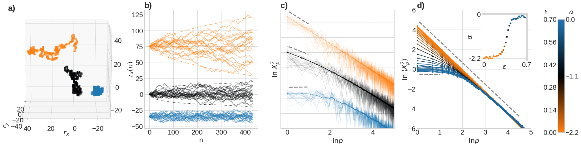
To test our hypotheses, we simulated single ISAW on the cubic lattice Tesi et al. 1996 and sampled conformations thanks to the Metropolis algorithm with reptation moves Wall and Mandel 1975. We performed simulations for ranging from 100 to 3000, and in the range 0.0–0.99. For each , 32000 statistically independent conformations are recorded. Figure 1-a shows typical conformations for the case and three different . The three spatial components are DCT transformed and their square amplitudes are summed to obtain their DCT spectra, as shown in Figure 1-c. For any given , we average over the set of configurations to obtain the corresponding PSD (thick lines in Figure 1-c). Figure 1-d shows the resulting PSDs for different values of and for the given .
The results confirm both our predictions. First, for small values of the interaction parameter , the PSDs display the expected scaling of Eq. (3), corresponding to a slope of in the log-log representation. Second, in the large region, the spatial trajectories clearly show the effect of confinement into the globule volume (Figure 1-b). Correspondingly, the low modes are strongly attenuated, leading to a rather flat spectrum, in agreement with our prediction (4).
We aimed to compare the scaling of to previous results, typically defined either by the vanishing of the second virial coefficient Grassberger and Hegger 1995, by the condition of divergent specific heat Vogel et al. 2007, or by a specific scaling of Rampf et al. 2006. In Ref. Vogel et al. 2007, Vogel et al. 2007 show by on-lattice simulations that the boundary between the two phases is best fitted by a function of the form . We here propose two different definitions for the phase transition critical line. The first one is simply given by the inflection points of the sigmoid functions. The corresponding points are very well-fitted by (Figure 2, circles, and Table S1). A second, more physical definition of a transition line is given by the that maximizes the fluctuations of our order parameter . Indeed, the relative standard deviation displays a sharp peak at the transition (meaning that the conformation of the polymer itself largely fluctuates) as shown by the inset of Figure 2. The corresponding maxima are again best fitted by (Figure 2, triangles and Table S1).
Interestingly, both and correspond to values of close to (black region) and are therefore far from , associated with RW-like configurations usually identified with the -point conditions. Our results show, instead, that these RW-like conditions do not appear at the crossover, but are rather located in the coil region of the phase diagram. More precisely, the condition is met at about (blue diamonds in Figure 2) and indeed corresponds to a PSD decreasing as over a wide -region (Figure S1). The corresponding curve is also fitted by a function (although with negligible , see Table S1; blue line in Figure 2). As expected, however, the asymptotic is virtually the same for the three critical curves , and and converge to the well established thermodynamic limit value of , in agreement with previous numerical estimates Grassberger and Hegger 1995; Vogel et al. 2007.
The existence of two distinct critical lines was already pointed out by des Cloizeaux and Jannink 1991 des Cloizeaux and Jannink 1991, but not clearly illustrated by numerical experiments, to the best of our knowledge. As a corollary message of our work, we confirm therefore that the conformation of a polymer of finite-size at the coil-globule transition is not reducible to a pure random walk. The very accurate phase diagrams obtained by spectral analysis validates it as a new, efficient and parsimonious method in polymer studies, neglected until now despite its very classical basis.
With our general hypotheses confirmed, we address the important issue of characterizing the coil-globule transition. Inspired by our previous observations on the low limit, we define as a new order parameter the log-log slope at
| (5) |
For the case of Figure 1-d, clearly performs a continuous transition from the typical SAW exponent to (inset). The width of the transition region depends, however, on . The curves, for all and , have been fitted by a 4-parameter sigmoid function (Figure 2, top panel), and all indeed interpolate between the two limiting values and . The fact that these limiting values are independent of and makes of an excellent order parameter for assessing the polymer state, as it can be applied to each single polymer configuration set and without the need of any information about these two parameters. The bottom panel of Figure 2 shows a color plot of as a function of and where colors span from orange, for , to blue for . The typical finite-size crossover region (in black) is clearly visible, allowing the definition of a critical transition line .
As a last, but most important point, the fact that our order parameter can be calculated on the basis of the first two spectral modes opens the possibility of experimentally assessing the state of a polymer from a very reduced and accessible information. The argument relies on a well-known property of the PSD: In order to get access to the first modes, it is indeed in principle sufficient to record the positions of distinguishable monomers, equally spaced along the polymer and covering the whole chain, meaning that the determination of would in theory require the knowledge of only 3 positions along the full polymer.
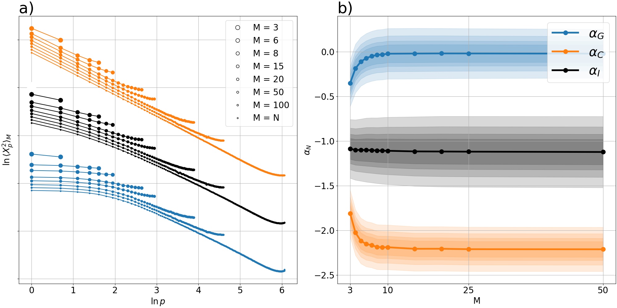
We tested the efficiency of our approach on decimated polymer chains, i.e., reduced signals where the positions of only equally spaced monomers are retained. We decimated down to , an extreme condition of particular interest from the experimental point of view since, in this case, time tracking can also be achieved without much difficulty Chen et al. 2018; Sato et al. 2020; Eykelenboom and Tanaka 2020 so that time averages can be used instead of ensemble averages. Figure 3-a shows examples of PSD obtained for different choices of . Extreme decimation () alters the first modes. As a consequence, the asymptotic values of the sigmoidal corresponding to ”pure” coils () and globules () vary, so that it is necessary to provide reference values for these limit slopes as a function of . We give these values in Figure 3-b and in the Table S2. Noteworthy, the asymptotic values for coils and globules remain well apart down to even for relatively low statistical sampling meaning that the arrangement of monomers on large scales is detectable whatever the sampling.
Once these -dependent limit values obtained, the order parameter can be normalized as so to span from -1 to 1. In this way, equivalent sigmoids are independent of Figure S2. For sufficiently large samples, even an extreme decimation with allows a very accurate reconstruction of the phase diagram (Figure S3). The critical line matches that of the complete chain (white line in Figure S3 and Table S3). The robustness of the proposed approach against variations in the size of the statistical sample is explored in Figure S4 showing that the universal character of the parameter potentially outperforms any other method aiming at determining in which phase a polymer in given conditions falls.
These results have relevant implications in the context of the study of chromatin. The characterization of the multiscale folding state of chromosomes is a crucial, issue since it likely determines its the biological activity. This is made evident from the strong progression of experimental methods to characterize this folding and their impact on the understanding of genetic regulation mechanisms Jerkovic´ and Cavalli 2021. Very recently, microscopy-based techniques allow for the first time the visualization of this polymer spatial trajectory by sequential labeling and imaging of multiple loci in a collection of fixed nuclei Cardozo Gizzi et al. 2019; Mateo et al. 2019; et al. 2020; Su et al. 2020. This results in configuration sets, sampled with a resolution ranging from 3 to several hundreds of points, which are for the moment difficult to analyze, the most frequent approaches being the reconstruction of parameters that were already obtainable with previous techniques. There is therefore a clear need for efficient methods to process this new data to the fullest and without loss of information. Our method of spectral analysis precisely fills this gap with a physically proven approach. Finally, we underline the very broad scope of this spectral approach, which extends far beyond the pure coil and globule. One can easily predict a specific spectral signature for fractal globules, loops, stretched polymers or a variety of multifractal configurations, potentially also interesting for the study of biopolymers.
Acknowledgements.
The authors would like to acknowledge networking support by the EUTOPIA COST Action CA17139. This work has been partially supported by the ANR project ANR-19-CE45-0016. Vincent Dahirel and Jean-Marc Victor are warmly acknowledged for their constant support and insightful advice.References
- Lesage et al. (2019) A. Lesage, V. Dahirel, J.-M. Victor, and M. Barbi, Epigenetics & Chromatin 12 (2019), 10.1186/s13072-019-0269-6.
- Doi and Edwards (1988) M. Doi and S. Edwards, The Theory of Polymer Dynamics, International series of monographs on physics (Clarendon Press, 1988).
- Socol et al. (2019) M. Socol, R. Wang, D. Jost, P. Carrivain, C. Vaillant, E. L. Cam, V. Dahirel, C. Normand, K. Bystricky, J.-M. Victor, O. Gadal, and A. Bancaud, Nucleic Acids Research 47, 6195 (2019).
- Rouse (1953) P. E. Rouse, The Journal of Chemical Physics 21, 1272 (1953).
- Makhoul (1980) J. Makhoul, IEEE Transactions on Acoustics, Speech, and Signal Processing 28, 27 (1980).
- Grosberg and Khokhlov (1994) A. Y. Grosberg and A. R. Khokhlov, Statistical Physics of Macromolecules, AIP series in polymers and complex materials (AIP Press, 1994).
- Krapf et al. (2018) D. Krapf, E. Marinari, R. Metzler, G. Oshanin, X. Xu, and A. Squarcini, New Journal of Physics 20, 023029 (2018).
- Panja and Barkema (2009) D. Panja and G. T. Barkema, The Journal of Chemical Physics 131, 154903 (2009).
- Slade (2019) G. Slade, Proceedings of the Royal Society A: Mathematical, Physical and Engineering Sciences 475, 20180549 (2019).
- Peliti (1986) L. Peliti, “Random walks with memory,” in Fractals in physics, edited by L. Pietronero and E. Tosatti (Elsevier, Amsterdam: North Holland, 1986) p. 73.
- de Gennes (1979) P.-G. de Gennes, Scaling concepts in polymer physics (Cornel University Press, 1979).
- Grassberger and Hegger (1995) P. Grassberger and R. Hegger, The Journal of Chemical Physics 102, 6881 (1995).
- Vogel et al. (2007) T. Vogel, M. Bachmann, and W. Janke, Physical Review E 76 (2007), 10.1103/physreve.76.061803.
- Caré et al. (2014) B. R. Caré, P. Carrivain, T. Forné, J.-M. Victor, and A. Lesne, Communications in Theoretical Physics 62, 607 (2014).
- Tesi et al. (1996) M. C. Tesi, E. J. J. van Rensburg, E. Orlandini, and S. G. Whittington, Journal of Statistical Physics 82, 155 (1996).
- Wall and Mandel (1975) F. T. Wall and F. Mandel, The Journal of Chemical Physics 63, 4592 (1975).
- Rampf et al. (2006) F. Rampf, K. Binder, and W. Paul, Journal of Polymer Science Part B: Polymer Physics 44, 2542 (2006).
- des Cloizeaux and Jannink (1991) J. des Cloizeaux and G. Jannink, Polymers in solution. Their modelling and structure (Oxford university press, New York, 1991).
- Chen et al. (2018) H. Chen, M. Levo, L. Barinov, M. Fujioka, J. B. Jaynes, and T. Gregor, Nature Genetics 50, 1296 (2018).
- Sato et al. (2020) H. Sato, S. Das, R. H. Singer, and M. Vera, Annual Review of Biochemistry 89, 159 (2020).
- Eykelenboom and Tanaka (2020) J. K. Eykelenboom and T. U. Tanaka, Cell Cycle 19, 1422 (2020).
- Jerkovic´ and Cavalli (2021) I. Jerkovic´ and G. Cavalli, Nature Reviews Molecular Cell Biology 22, 511–528 (2021).
- Cardozo Gizzi et al. (2019) A. M. Cardozo Gizzi, D. I. Cattoni, J.-B. Fiche, S. M. Espinola, J. Gurgo, O. Messina, C. Houbron, Y. Ogiyama, G. L. Papadopoulos, G. Cavalli, M. Lagha, and M. Nollmann, Molecular Cell 74, 212 (2019).
- Mateo et al. (2019) L. Mateo, S. Murphy, A. Hafner, I. Cinquini, C. Walker, and A. Boettiger, Nature 568 (2019).
- et al. (2020) H. Q. N. et al., Nature methods 17, 822 (2020).
- Su et al. (2020) J.-H. Su, P. Zheng, S. Kinrot, B. Bintu, and X. Zhuang, Cell 182, 1641 (2020).