跳到论文正文
W Papers独立论文阅读器 arXiv:2107.07880 论文正文 计算阅读时间 · 0%
引用这篇论文根据当前论文元数据生成,正式投稿前建议核对。


License: arXiv.org perpetual non-exclusive license
arXiv:2107.07880v1 [hep-lat] 31 May 2021

Renormalization of (2+1)​D(2+1)D scalar Weyl spinors interactions on lattices
using the Clifford groups

Sadataka Furui Affiliation: (Formerly) Graduate School of Science and Engineering, Teikyo University, Utsunomiya, 320 Japan Email: furui@umb.teikyo-u.ac.jp
August 11, 2026
Abstract

We consider symplectic quaternions instead of unitary spinors sitting on a lattice, and calculate the fixed point Wilson action on a finite 2​D2D plane expanded by u1​a​e1+u2​a​e2u_{1}ae_{1}+u_{2}ae_{2} and on two 2​D2D planes separated by a​e1∧e2ae_{1}\wedge e_{2}. Only the nearlest neighbor interactions are considered. Following Migdal and Kadanoff, we perform the renormalization of the Wilson action by making the lattice spacing (12)h​a(\frac{1}{2})^{h}a (h=0,⋯,11)(h=0,\cdots,11), in order to simulate bosonic and solitonic phonon propagation in materials. Renormalization group method of Benfatto and Gallavotti for (2+1)​D(2+1)D scalar ϕ4\phi^{4} system for sound propagation in Fermi sea is applied and feasibility of numerical simulation is discussed.

Keywords: 
Renormalization group and Soliton

I Introduction

In SF21, an outline of performing a simulation of phonetic solitons propagating on (2+1)​D(2+1)D plane was proposed. We start from 4×44\times 4 lattices surrounded by Clifford pairs, and by adopting the renormalization group method, calculate the correlations of ultra-sonic phonetic solitons.

A main difference from standard methods is on each lattice site quatrernions following symplectic groups are sitting., not spin following unitary groups.

We considered the fixed point Wilson actions in one loop adopted by deGrand et al.DGHHN95. They considered in the (3+1)​D(3+1)D lattice, 28 Fixed point (FP) actions of length less than or equal to 8 lattice lengths. We classify the FP actions to L​o​o​p​cLoopc which consist of loops on one 2​D2D plane expanded by e1e_{1} and e2e_{2}, and L​o​o​p​dLoopd which consist of loops on two parallel 2​D2D planes connected by two links in the direction e1∧e2e_{1}\wedge e_{2} and in the direction e2∧e1e_{2}\wedge e_{1}. The L​o​o​p​1,2,5,6,11,12,18Loop1,2,5,6,11,12,18 and 2828 belong to the L​o​o​p​CLoopC and the L​o​o​p​3,4,7,8,9,10,13,14,15,16,17Loop3,4,7,8,9,10,13,14,15,16,17 and 26,2726,27 belong to the L​o​o​p​DLoopD. L​o​o​p​19,⋯,25Loop19,\cdots,25 are irrelevant in (2+1)​D(2+1)D.

In abstract graph theory of LuescherLuescher86 a loop in a graph is a non-empty subset of lines with the property that there exists a sequence v1,⋯,vNv_{1},\cdots,v_{N} of pairwise different vertices and a labelling ℓ1,⋯,ℓN\ell_{1},\cdots,\ell_{N} of the lines in a loop, such that vk,vk+1v_{k},v_{k+1} are the end points of ℓk\ell_{k} (k=1,⋯,N−1)(k=1,\cdots,N-1) and vN,v1v_{N},v_{1} are end points of ℓN\ell_{N}. On every loop there are two orientations, and a crossing of two loops produces a new vertex.

In this sence, the L​o​o​p​28Loop28 is not a proper loop. In DGHHN95, the loop did not play important roles, and we also observed that the eigenvalues of the action are large. We did not consider the L​o​o​p​26Loop26 and 2727 which are shown in Fig.1 since eigenvalues were large, but we consider these loops in (2+1)​D(2+1)D space, since they are proper.

Refer to caption
Refer to caption
Figure 1: Loop26 (left) and Loop27 (right).

Depending on the direction of the link between two planes, we consider paths

L​o​o​p​26​αLoop26\alpha: 𝐮→𝐮+a​e1→{\bf u}\to{\bf u}+ae_{1}\to 𝐮+a​e1+a​e2→{\bf u}+ae_{1}+ae_{2}\to 𝐮+a​e1+a​e2+a​e1∧e2→{\bf u}+ae_{1}+ae_{2}+ae_{1}\wedge e_{2}\to 𝐮+a​e1+a​e1∧e2→{\bf u}+ae_{1}+ae_{1}\wedge e_{2}\to 𝐮+a​e1→{\bf u}+ae_{1}\to 𝐮+a​e1+a​e2→{\bf u}+ae_{1}+ae_{2}\to 𝐮+a​e2→{\bf u}+ae_{2}\to 𝐮{\bf u}, and

L​o​o​p​26​βLoop26\beta: 𝐮→𝐮+a​e1→{\bf u}\to{\bf u}+ae_{1}\to 𝐮+a​e1+a​e2→{\bf u}+ae_{1}+ae_{2}\to 𝐮+a​e1+a​e2+a​e2∧e1→{\bf u}+ae_{1}+ae_{2}+ae_{2}\wedge e_{1}\to 𝐮+a​e1+a​e2∧e1→{\bf u}+ae_{1}+ae_{2}\wedge e_{1}\to 𝐮+a​e1→{\bf u}+ae_{1}\to 𝐮+a​e1+a​e2→{\bf u}+ae_{1}+ae_{2}\to 𝐮+a​e2→{\bf u}+ae_{2}\to 𝐮{\bf u}.

Similarly the paths

L​o​o​p​27​αLoop27\alpha: 𝐮→𝐮+a​e1→{\bf u}\to{\bf u}+ae_{1}\to 𝐮+a​e1+a​e2→{\bf u}+ae_{1}+ae_{2}\to 𝐮+a​e1+a​e2+a​e1∧e2→{\bf u}+ae_{1}+ae_{2}+ae_{1}\wedge e_{2}\to 𝐮+a​e1+a​e1∧e2→{\bf u}+ae_{1}+ae_{1}\wedge e_{2}\to 𝐮+a​e1∧e2→{\bf u}+ae_{1}\wedge e_{2}\to 𝐮+a​e2+a​e1∧e2→{\bf u}+ae_{2}+ae_{1}\wedge e_{2}\to 𝐮+a​e2→{\bf u}+ae_{2}\to 𝐮{\bf u}, and

L​o​o​p​27​βLoop27\beta: 𝐮→𝐮+a​e1→{\bf u}\to{\bf u}+ae_{1}\to 𝐮+a​e1+a​e2→{\bf u}+ae_{1}+ae_{2}\to 𝐮+a​e1+a​e2+a​e2∧e1→{\bf u}+ae_{1}+ae_{2}+ae_{2}\wedge e_{1}\to 𝐮+a​e1+a​e2∧e1→{\bf u}+ae_{1}+ae_{2}\wedge e_{1}\to 𝐮+a​e2∧e1→{\bf u}+ae_{2}\wedge e_{1}\to 𝐮+a​e2+a​e2∧e1→{\bf u}+ae_{2}+ae_{2}\wedge e_{1}\to 𝐮+a​e2→{\bf u}+ae_{2}\to 𝐮{\bf u}.

In the two loops α\alpha and β\beta, the blue circle and the red circle are to be interchanged.

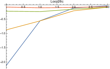
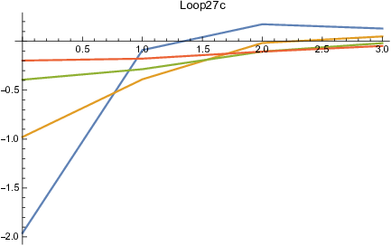
The eigenvalues of loops have dependence on the direction of paths. Difference of eigenvalues between L​o​o​p​26​αLoop26\alpha and L​o​o​p​26​βLoop26\beta is larger than that of L​o​o​p​27​αLoop27\alpha and L​o​o​p​27​βLoop27\beta. Their eigenvalues are about the same as those of L​o​o​p​28Loop28.

The dependence of eigenvalues on the direction of e1∧e2e_{1}\wedge e_{2} shows a presence of time reversal symmetric but rotational symmetry breaking phase.

We evaluate Wilson’s optimum plaquet actions by making a linear combination of eigenvalues of selected FP actions.

The structure of this presentation is as follows. In Sec. II, we compare eigenvalues χ⁡(L(h))\chi(L^{(h)}) of L​o​o​p​CLoopC and L​o​o​p​DLoopD for a lattice spacing aa used in SF20 and a/2a/2. The similar analysis for the trace of link variables are given in Sec. III. In Sec. IV, a perspective of the renormalization group analysis using supercomputer are given.

II Lattice spacing dependence of eigenvalues of plaquettes

We consider the case in which the spacing between the lattice Δ​x=ei4\Delta x=\frac{e_{i}}{4} which is called L​o​o​p​CLoopC and they are Δ​x=ei8\Delta x=\frac{e_{i}}{8} which are called L​o​o​p​DLoopD.

II.1 Paths on one 2DD plane expanded by e1e_{1} and e2e_{2}

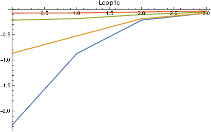
The L​o​o​p​1Loop1 consists of 4 sides of a square, whose eigenvalue is the smallest among the FP actions. We characterized the path by 𝐮→{\bf u}\to 𝐮+14​e1→{\bf u}+\frac{1}{4}e_{1}\to 𝐮+e14+e24→{\bf u}+\frac{e_{1}}{4}+\frac{e_{2}}{4}\to 𝐮+e24→{\bf u}+\frac{e_{2}}{4}\to 𝐮\bf u where 𝐮{\bf u} are mesh points (u1​e1+u2​e2)(u_{1}e_{1}+u_{2}e_{2}), 0≤u1,u2≤30\leq u_{1},u_{2}\leq 3 (ui∈𝐙u_{i}\in{\bf Z}). We call the path L​o​o​p​1​cLoop1c.

We compare eigenvalues of the path of 𝐮→{\bf u}\to 𝐮+18​e1→{\bf u}+\frac{1}{8}e_{1}\to 𝐮+e18+e28→{\bf u}+\frac{e_{1}}{8}+\frac{e_{2}}{8}\to 𝐮+e28→{\bf u}+\frac{e_{2}}{8}\to 𝐮−18​e2→{\bf u}-\frac{1}{8}e_{2}\to 𝐮\bf u, which we call L​o​o​p​1​dLoop1d.

In the left figure of Fig.2, eigenvalues of u1=0​(b​l​u​e),1​(o​r​a​n​g​e),2​(g​r​e​e​n),3​(r​e​d)u_{1}=0(blue),1(orange),2(green),3(red) as a function of u2u_{2} are plotted, and in the right figure of Fig.2, eigenvalues of u1=0,12,1,32,2,52,3u_{1}=0,\frac{1}{2},1,\frac{3}{2},2,\frac{5}{2},3 as a function of u2u_{2} are plotted. When the lattice spacing is smaller, eigenvalues are smaller.

Refer to caption
Refer to caption
Figure 2: Absolute values of eigenvalues for fixed u1u_{1} in Loop1c(left) and in Loop1d (right).

The eigenvalues of L​o​o​p​28Loop28 are shown in Fig.3.The loop is not proper in the sence of LuescherLuescher86. Fluctuations are large for small 𝐮{\bf u} or in infrared regions.

Refer to caption
Refer to caption
Figure 3: Absolute values of eigenvalues for fixed u1u_{1} in Loop28c(left) and in Loop28d(right).

The eigenvalues of L​o​o​p​2Loop2 are shown in Fig.4.Eigenvalues of the smaller lattice spacing L​o​o​p​2​dLoop2d is smaller than those of L​o​o​p​s​2​cLoops2c.

Refer to caption
Refer to caption
Figure 4: Absolute values of eigenvalues for a fixed u1u_{1} in Loop2c(left) and in Loop2d(right)

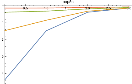
The eigenvalues of L​o​o​p​5Loop5 are shown in Fig.5. The L​o​o​p​5Loop5 has a bending point of the path at the center of the loop. It produces a large eigenvalues for small u1u_{1}.

Refer to caption
Refer to caption
Figure 5: Absolute values of eigenvalues for a fixed u1u_{1} in Loop5c(left) and in Loop5d(right) .

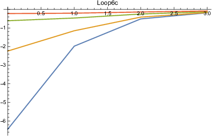
The eigenvalues of L​o​o​p​6Loop6 are shown in Fig.6.They have 𝐮{\bf u} dependence in the infrared region.

Refer to caption
Refer to caption
Figure 6: Absolute values of eigenvalues for a fixed u1u_{1} in Loop6c (left) and in Loop6d (right).

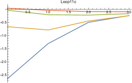
The eigenvalues of L​o​o​p​11Loop11 are shown in Fig.7.The L​o​o​p​11Loop11 has a bending due to presence of overlapping links in the center.

Refer to caption
Refer to caption
Figure 7: Absolute values of eigenvalues for a fixed u1u_{1}in Loop11c (left) and in Loop11d (right).

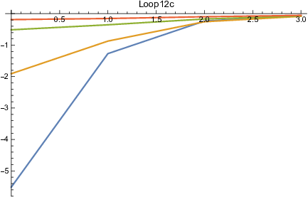
The eigenvalues of L​o​o​p​12Loop12 are shown in Fig.8, The L​o​o​p​12Loop12 is similar to the L​o​o​p​5Loop5, but there is a self-crossing of two long links at the center. The 𝐮\bf u dependence of eigenvalues of L​o​o​p​5Loop5 and L​o​o​p​12Loop12 are similar, but absolute values of eigenvalues of L​o​o​p​12Loop12 are smaller, due to presence of long links. In the (3+1)​D(3+1)D lattice simulation of DGHHN95, the L​o​o​p​5Loop5 is more effective than L​o​o​p​12Loop12.

Refer to caption
Refer to caption
Figure 8: Absolute values of eigenvalues for a fixed u1u_{1} in Loop12c (left) and in Loop12d(right). .

In SF21, the starting point of theL​o​o​p​18Loop18 was chosen to be same as the L​o​o​p​1Loop1, and only the scale was changed. In this paper we replace the verices as those of the paper DGHHN95,

L​18​[u1,u2]=t​1​[−14,u1+14,u2]×t​2​[−12,u1+14,u2+12]×t​1​[−12,u1+14,u2+12]×t​2​[12,u1+14,u2]×t​1​[14,u1,u2].L18[u_{1},u_{2}]=t1[-\frac{1}{4},u_{1}+\frac{1}{4},u_{2}]\times t2[-\frac{1}{2},u_{1}+\frac{1}{4},u_{2}+\frac{1}{2}]\times t1[-\frac{1}{2},u_{1}+\frac{1}{4},u_{2}+\frac{1}{2}]\times t2[\frac{1}{2},u_{1}+\frac{1}{4},u_{2}]\times t1[\frac{1}{4},u_{1},u_{2}].

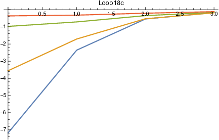
The eigenvalues of the new L​o​o​p​18Loop18 and its lattice scalings halved are shown in Fig.9.The L​o​o​p​18Loop18 contains long straight links parallel to e2e_{2}.

Refer to caption
Refer to caption
Figure 9: Absolute values of eigenvalues for a fixed u1u_{1} in Loop18c (left) and in Loop18d (right).

II.2 Paths on two planes connected by e1∧e2e_{1}\wedge e_{2}

When there are links between two 2​D2D planes, a proplem of choice of scale of length between the two 2D planes appears. We leave it as a future study, and calculate eigenvalues using the same lattice spacing between the 2D planes and on the 2D plane.

The paths on two planes we considered in SF20 were restricted to α\alpha type. Since eigenvalues in the large 𝐮\bf u region are almost independent of α\alpha and β\beta, we restrict loops to be α\alpha type and consider β\beta type near the final stage of MonteCarlo simulation.

The path of L​o​o​p​3​cLoop3c consists of 𝐮→𝐮+14​e1→{\bf u}\to{\bf u}+\frac{1}{4}e_{1}\to 𝐮+14​e1+14​e2→{\bf u}+\frac{1}{4}e_{1}+\frac{1}{4}e_{2}\to 𝐮+14​e1+14​e2+14​e1∧e2→{\bf u}+\frac{1}{4}e_{1}+\frac{1}{4}e_{2}+\frac{1}{4}e_{1}\wedge e_{2}\to 𝐮+14​e1+14​e1∧e2→{\bf u}+\frac{1}{4}e_{1}+\frac{1}{4}e_{1}\wedge e_{2}\to 𝐮+14​e1∧e2→{\bf u}+\frac{1}{4}e_{1}\wedge e_{2}\to 𝐮{\bf u}.

The path of L​o​o​p​3​dLoop3d consists of 𝐮→𝐮+18​e1→{\bf u}\to{\bf u}+\frac{1}{8}e_{1}\to 𝐮+18​e1+18​e2→{\bf u}+\frac{1}{8}e_{1}+\frac{1}{8}e_{2}\to 𝐮+18​e1+18​e2+18​e1∧e2→{\bf u}+\frac{1}{8}e_{1}+\frac{1}{8}e_{2}+\frac{1}{8}e_{1}\wedge e_{2}\to 𝐮+18​e1+18​e1∧e2→{\bf u}+\frac{1}{8}e_{1}+\frac{1}{8}e_{1}\wedge e_{2}\to 𝐮+18​e1∧e2→{\bf u}+\frac{1}{8}e_{1}\wedge e_{2}\to 𝐮{\bf u}.

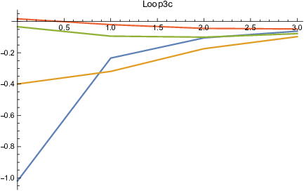
The eigenvalues of L​o​o​p​3Loop3 are shown in Fig.10 .We observe the eigenvalues of action of L​o​o​p​3Loop3 is roughly about twice of those of L​o​o​p​1Loop1.

Refer to caption
Refer to caption
Figure 10: Absolute values of eigenvalues for a fixed u1u_{1} in Loop3c (left) and in Loop3d(right).

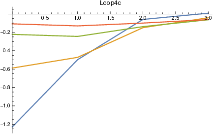
The eigenvalues of L​o​o​p​4Loop4 are shown in Fig.11.

Refer to caption
Refer to caption
Figure 11: Absolute values of eigenvalues for a fixed u1u_{1} in Loop4c (left) and in Loop4d(right).

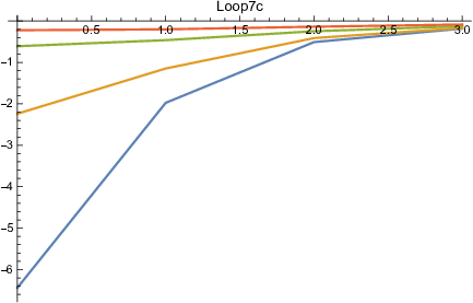
The eigenvalues of L​o​o​p​7Loop7 are shown in Fig.12.

Refer to caption
Refer to caption
Figure 12: Absolute values of eigenvalues for a fixed u1u_{1} in Loop7c (left) and in Loop7d (right).

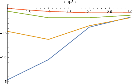
The eigenvalues of L​o​o​p​8Loop8 are shown in Fig.13.

Refer to caption
Refer to caption
Figure 13: Absolute values of eigenvalues for a fixed u1u_{1} in Loop6c (left) and in Loop8d(right).

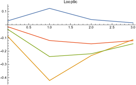
The eigenvalues of L​o​o​p​9Loop9 are shown in Fig.14 .

Refer to caption
Refer to caption
Figure 14: Absolute values of eigenvalues for a fixed u1u_{1} in Loop9c(left) and in Loop9d(right).

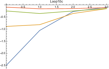
The eigenvalues of L​o​o​p​10Loop10 are shown in Fig.15.

Refer to caption
Refer to caption
Figure 15: Absolute values of eigenvalues for a fixed u1u_{1} in Loop10c(left) and in Loop10d(right).

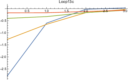
The eigenvalues of L​o​o​p​13Loop13 are shown in Fig.16.

Refer to caption
Refer to caption
Figure 16: Absolute values of eigenvalues for a fixed u1u_{1} in Loop13c (left) and in Loop13d(right).

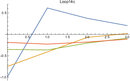
The eigenvalues of L​o​o​p​14Loop14 are shown in Fig.17 .

Refer to caption
Refer to caption
Figure 17: Absolute values of eigenvalues for a fixed u1u_{1} in Loop14c (left) and in Loop14d(right).

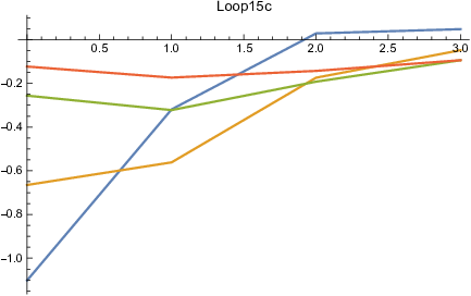
The eigenvalues of L​o​o​p​15Loop15 are shown in Fig.18.

Refer to caption
Refer to caption
Figure 18: Absolute values of eigenvalues for a fixed u1u_{1} in Loop15c(left) and in Loop15d (right).

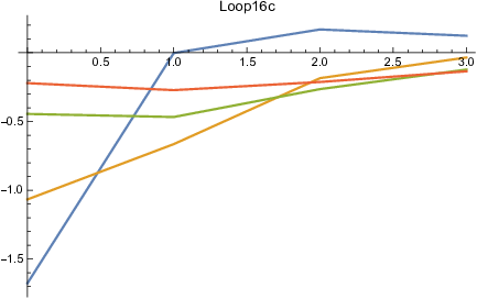
The eigenvalues of L​o​o​p​16Loop16 are shown in Fig.19 .

Refer to caption
Refer to caption
Figure 19: Absolute values of eigenvalues for a fixed u1u_{1} in Loop16c(left) and in Loop16d(right).

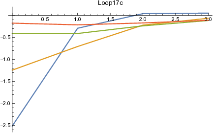
The eigenvalues of L​o​o​p​17Loop17 are shown in Fig.20.

Refer to caption
Refer to caption
Figure 20: Absolute values of eigenvalues for a fixed u1u_{1} in Loop17c (left) and in Loop17d(right).

The eigenvalues of the L​o​o​p​26​αLoop26\alpha and L​o​o​p​26​βLoop26\beta of a=1/8a=1/8 are shown in Fig.21

Refer to caption
Refer to caption
Figure 21: Absolute values of eigenvalues for a fixed u1u_{1} in Loop26α\alpha(left) and in Loop26β\beta (right).

The eigenvalues of the L​o​o​p​27​αLoop27\alpha and L​o​o​p​27​βLoop27\beta are shown in Fig.22

Refer to caption
Refer to caption
Figure 22: Absolute values of eigenvalues for a fixed u1u_{1} in Loop27d (left) and in Loop27f(right).

III Lattice spacing dependence of traces of link variables

In Clifford algebra, transformation of a coordinate XX is represented byPorteous95

(acbd)​(xx​x−1x−)​(d−c−b−a−)=λ​(x′x′​x′−1x′⁣−)\left(\begin{array}[]{cc}a&c\\ b&d\end{array}\right)\left(\begin{array}[]{cc}x&xx^{-}\\ 1&x^{-}\end{array}\right)\left(\begin{array}[]{cc}d^{-}&c^{-}\\ b^{-}&a^{-}\end{array}\right)=\lambda\left(\begin{array}[]{cc}x^{\prime}&x^{\prime}{x^{\prime}}^{-}\\ 1&{x}^{\prime-}\end{array}\right)

and the term x​x−xx^{-} yields link products.

In lattice simulations of scalar fields, we consider Feynman path integrals is Z=∫[𝑑ψ]​e−SZ=\int[d\psi]e^{-S} with 𝐱=a⁡(u1​e1+u2​e2)+a​u3​e1∧e2{\bf x}=a(u_{1}e_{1}+u_{2}e_{2})+au_{3}e_{1}\wedge e_{2}, −N/2<u1,u2,u3≤N/2-N/2<u_{1},u_{2},u_{3}\leq N/2, μ=1,2,3\mu=1,2,3. N∼211=2048N\sim 2^{11}=2048. The scale of e1∧e2e_{1}\wedge e_{2} is chosen to be the same as e1,e2e_{1},e_{2}, for Wilson loops, but it can be complex for Polyakov loops.

The expectation values of Wilson or Polyakov action SS consists of eigenvalues of left lower components of the Loop matrices L​k​[u1,u2]Lk[u_{1},u_{2}] where kk specifies the FP actions of DGHHN95, and the trace of D​𝐒​(L​k​[u1,u2])D{\bf S}(Lk[u_{1},u_{2}]) which consists of the sum of d​S1dS_{1} and d​S2dS_{2} along the loops

The 4×44\times 4 matrix of the L​o​o​p​1Loop1 contribution

D​𝐒​(L​1​[u1,u2])=d​S1​[u1,u2]+d​S2​[u1+a,u2]−d​S1​[u1+a,u2+a]−d​S2​[u1,u2+a]D{\bf S}(L1[u_{1},u_{2}])=dS_{1}[u_{1},u_{2}]+dS_{2}[u_{1}+a,u_{2}]-dS_{1}[u_{1}+a,u_{2}+a]-dS_{2}[u_{1},u_{2}+a]

has non-zero components in the right upper component. We measure the trace of the 2×22\times 2 matrices.

In the case of L​o​o​p​2Loop2,

D​𝐒​(L​2​[u1,u2])=d​S1​[u1,u2]+2​d​S2​[u1+a,u2]−d​S1​[u1+a,u2+2​a]−2​d​S2​[u1,u2+2​a]D{\bf S}(L2[u_{1},u_{2}])=dS_{1}[u_{1},u_{2}]+2dS_{2}[u_{1}+a,u_{2}]-dS_{1}[u_{1}+a,u_{2}+2a]-2dS_{2}[u_{1},u_{2}+2a]

has non-zero components only in the right upper corner.

III.1 Paths on one 2DD plane expanded by e1e_{1} and e2e_{2}

The traces of the 2×22\times 2 matrix, which is twice the real part of the diagonal component in the case of L​o​o​p​1Loop1 as a function of u2u_{2} for fixed u1u_{1} are shown in Fig.23.

Refer to caption
Refer to caption
Figure 23: Trace of d​𝐒​(L​1​[u1,u2])d{\bf S}(L1[u_{1},u_{2}]) for Δ​ui=1\Delta{u_{i}}=1(left) and Δ​ui=12\Delta{u_{i}}=\frac{1}{2}(right). (i=1,2i=1,2)

The traces of the matrix in the case of L​o​o​p​2Loop2 are shown in Fig.24.

Refer to caption
Refer to caption
Figure 24: Trace of d​𝐒​(L​2​[u1,u2])d{\bf S}(L2[u_{1},u_{2}]) for Δ​ui=1\Delta{u_{i}}=1(left) and Δ​ui=12\Delta{u_{i}}=\frac{1}{2}(right). (OPENi=1,2)i=1,2)

The traces of the matrix in the case of L​o​o​p​5Loop5 are shown in Fig.25.

Refer to caption
Refer to caption
Figure 25: Trace of d​𝐒​(L​5​[u1,u2])d{\bf S}(L5[u_{1},u_{2}]) for Δ​ui=1\Delta{u_{i}}=1(left) and Δ​ui=12\Delta{u_{i}}=\frac{1}{2}(right). (OPENi=1,2)i=1,2)

The traces of the matrix in the case of L​o​o​p​5Loop5 are shown in Fig.26.

Refer to caption
Refer to caption
Figure 26: Trace of d​𝐒​(L​6​[u1,u2])d{\bf S}(L6[u_{1},u_{2}]) for Δ​ui=1\Delta{u_{i}}=1(left) and Δ​ui=12\Delta{u_{i}}=\frac{1}{2}(right). (OPENi=1,2)i=1,2)

The traces of the matrix in the case of L​o​o​p​11Loop11 are shown in Fig.27.

Refer to caption
Refer to caption
Figure 27: Trace of d​𝐒​(L​11​[u1,u2])d{\bf S}(L11[u_{1},u_{2}]) for Δ​ui=1\Delta{u_{i}}=1(left) and Δ​ui=12\Delta{u_{i}}=\frac{1}{2}(right). (OPENi=1,2)i=1,2)

The traces of the matrix in the case of L​o​o​p​12Loop12 are shown in Fig.28.

Refer to caption
Refer to caption
Figure 28: Trace of d​𝐒​(L​12​[u1,u2])d{\bf S}(L12[u_{1},u_{2}]) for Δ​ui=1\Delta{u_{i}}=1(left) and Δ​ui=12\Delta{u_{i}}=\frac{1}{2}(right). (OPENi=1,2)i=1,2)

The traces of the matrix in the case of L​o​o​p​18Loop18 are shown in Fig.29..

Refer to caption
Refer to caption
Figure 29: Trace of d​𝐒​(L​18​[u1,u2])d{\bf S}(L18[u_{1},u_{2}]) for Δ​ui=1\Delta{u_{i}}=1(left) and Δ​ui=12\Delta{u_{i}}=\frac{1}{2}(right). (OPENi=1,2)i=1,2)

III.2 Paths on two planes connected by e1∧e2e_{1}\wedge e_{2}

The traces of the matrix in the case of L​o​o​p​3Loop3 are shown in Fig.30.

Refer to caption
Refer to caption
Figure 30: Trace of d​𝐒​(L​3​[u1,u2])d{\bf S}(L3[u_{1},u_{2}]) for Δ​ui=1\Delta{u_{i}}=1(left) and Δ​ui=12\Delta{u_{i}}=\frac{1}{2}(right). (OPENi=1,2)i=1,2)

The traces of the matrix in the case of L​o​o​p​4Loop4 are shown in Fig.31.

Refer to caption
Refer to caption
Figure 31: Trace of d​𝐒​(L​4​[u1,u2])d{\bf S}(L4[u_{1},u_{2}]) for Δ​ui=1\Delta{u_{i}}=1(left) and Δ​ui=12\Delta{u_{i}}=\frac{1}{2}(right). (OPENi=1,2)i=1,2)

The traces of the matrix in the case of L​o​o​p​7Loop7 are shown in Fig.32.

Refer to caption
Refer to caption
Figure 32: Trace of d​𝐒​(L​7​[u1,u2])d{\bf S}(L7[u_{1},u_{2}]) for Δ​ui=1\Delta{u_{i}}=1(left) and Δ​ui=12\Delta{u_{i}}=\frac{1}{2} (right). (OPENi=1,2)i=1,2)

The traces of the matrix in the case of L​o​o​p​8Loop8 are shown in Fig.33.

Refer to caption
Refer to caption
Figure 33: Trace of d​𝐒​(L​8​[u1,u2])d{\bf S}(L8[u_{1},u_{2}]) for Δ​ui=1\Delta{u_{i}}=1(left) and Δ​ui=12\Delta{u_{i}}=\frac{1}{2} (right.) (OPENi=1,2)i=1,2)

The traces of the matrix in the case of L​o​o​p​9Loop9 are shown in Fig.34.

Refer to caption
Refer to caption
Figure 34: Trace of d​𝐒​(L​9​[u1,u2])d{\bf S}(L9[u_{1},u_{2}]) for Δ​ui=1\Delta{u_{i}}=1(left) and Δ​ui=12\Delta{u_{i}}=\frac{1}{2} (right). (OPENi=1,2)i=1,2)

The traces of the matrix in the case of L​o​o​p​10Loop10 are shown in Fig.35.

Refer to caption
Refer to caption
Figure 35: Trace of d​𝐒​(L​10​[u1,u2])d{\bf S}(L10[u_{1},u_{2}]) for Δ​ui=1\Delta{u_{i}}=1(left) and Δ​ui=12\Delta{u_{i}}=\frac{1}{2} (right). (OPENi=1,2)i=1,2)

The traces of the matrix in the case of L​o​o​p​13Loop13 are shown in Fig.36.

Refer to caption
Refer to caption
Figure 36: Trace of d​𝐒​(L​13​[u1,u2])d{\bf S}(L13[u_{1},u_{2}]) for Δ​ui=1\Delta{u_{i}}=1(left) and Δ​ui=12\Delta{u_{i}}=\frac{1}{2} (right). (OPENi=1,2)i=1,2)

The traces of the matrix in the case of L​o​o​p​14Loop14 are shown in Fig.37.

Refer to caption
Refer to caption
Figure 37: Trace of d​𝐒​(L​14​[u1,u2])d{\bf S}(L14[u_{1},u_{2}]) for Δ​ui=1\Delta{u_{i}}=1(left) and Δ​ui=12\Delta{u_{i}}=\frac{1}{2} (right). (OPENi=1,2)i=1,2)

The traces of the matrix in the case of L​o​o​p​15Loop15 are shown in Fig.38.

Refer to caption
Refer to caption
Figure 38: Trace of d​𝐒​(L​15​[u1,u2])d{\bf S}(L15[u_{1},u_{2}]) for Δ​ui=1\Delta{u_{i}}=1(left) and Δ​ui=12\Delta{u_{i}}=\frac{1}{2} (right). (OPENi=1,2)i=1,2)

The traces of the matrix in the case of L​o​o​p​16Loop16 are shown in Fig.39.

Refer to caption
Refer to caption
Figure 39: Trace of d​𝐒​(L​16​[u1,u2])d{\bf S}(L16[u_{1},u_{2}]) for Δ​ui=1\Delta{u_{i}}=1(left) and Δ​ui=12\Delta{u_{i}}=\frac{1}{2} (right). (OPENi=1,2)i=1,2)

The traces of the matrix in the case of L​o​o​p​17Loop17 are shown in Fig.40.

Refer to caption
Refer to caption
Figure 40: Trace of d​𝐒​(L​17​[u1,u2])d{\bf S}(L17[u_{1},u_{2}]) for Δ​ui=1\Delta{u_{i}}=1(left) and Δ​ui=12\Delta{u_{i}}=\frac{1}{2}(right). (OPENi=1,2)i=1,2)

The traces of the matrix in the case of L​o​o​p​26Loop26 are shown in Fig.41.

Refer to caption
Refer to caption
Figure 41: Trace of d​𝐒​(L​26​[u1,u2])d{\bf S}(L26[u_{1},u_{2}]) for Δ​ui=1\Delta{u_{i}}=1(left) and Δ​ui=12\Delta{u_{i}}=\frac{1}{2}(right). (OPENi=1,2)i=1,2)

The traces of the matrix in the case of L​o​o​p​27Loop27 are shown in Fig.42.

Refer to caption
Refer to caption
Figure 42: Trace of d​𝐒​(L​27​[u1,u2])d{\bf S}(L27[u_{1},u_{2}]) for Δ​ui=1\Delta{u_{i}}=1(left) and Δ​ui=12\Delta{u_{i}}=\frac{1}{2}(right). (OPENi=1,2)i=1,2)

IV Discussion and perspective

We expected that correlation of phonons and its time-reversed phonons propagating on a 2​D2D plane can be simulated by a model of Bosonic quasiparticle propagating in the Fermionic sea of Weyl spinors.

In an exploratory analysis using Clifford algebra, we observed that as the lattice spacing aa is halved, eigenvalues of the FP Wilson action and the trace of the matrix representing links of Loops surrounding each FP Wilson action are reduced. Monte-Carlo simulations using a small lattice constant aa will allow fixing the optimal Wilson action or the Polyakov action as a linear combination of the FP actions with correction terms derived by the renormalization group.

There are works on the study of Quantum spin systems associated with time translations and space translations of lattice spacesRobinson68; LR72. Solitons are integrable systems induced by nonlinear interactions. Detailed comparison between experiments and simulation will clarify the Kubo-Martin-Schwinger boundary condition.

We have a plan of reducing aa and perform the renormalization group analysis using supercomputers which allow parallel computations. Whether one can connects the chiral anomaly and grvitation alanomaly by simulating the ultrasonic waves remanis as a future study.

Acknowledgements.
I thank Dr. Serge DosSantos at INSA for valuable discussion and Prof. M. Arai for supports. Thanks are also due to the CMC of Osaka University for allowing use of super computers there, which were developed by CMC and Tokyo Institute of Technology.

References

  • (1) Sadataka Furui, Lattice simulation of (2+1)​D(2+1)D phonetic solitons and the Renormalization group, arXiv: 2105.06265[hep-lat].
  • (2) T.DeGrand, A. Hasenfrats, P. Hasenfratz, and F. Niedermayer, Non-perturbative tests of the fixed point action for SU(3) gauge theory, Nucl. Phys. B 454, 615-637 (1995); arXiv: hep-lat/9506031 (1995).
  • (3) M. Luescher, Volume Dependence of the Energy Spectrum in Massive Quantum Field Theories, I. Stable Particle States, Commun. Math. Phys. 104, 177-206 (1986).
  • (4) Michael Creutz, Quarks, gluons and lattices, Cambridge Monographs on Mathematical Physics, Cambridge (1983).
  • (5) P. Hasenfratz and F. Niedermayer, Fixed-Point Actions in 1-Loop Perturbation Theory, arXiv:hep-lat/9706002 v1 (1997).
  • (6) K.G. Wilson, Renormalization Group and Critical Phenomena, I. Renormalizatio Group and the Kadanoff Scaling Picture, Phys. Rev. B4(9) 3174-3183 (1971).
  • (7) K.G. Wilson, Renormalization Group and Critical Phenomena, II. Phase-Space Cell Analysis of Critical Behavior, Phys. Rev. B4(9) 3184-3205 (1971).
  • (8) Kenneth G. Wilson, Confinement of quarks, Phys. Rev. D 10,(8) 2445-2459 (1974).
  • (9) Giovanni Gallavotti, Renormalization theory and ultraviolet stability for scalar fields via renormalization group methods, Rev. Mod. Phys. 57, 471-562 (1985).
  • (10) G. Benefatto and G. Gallavotti, Renormalization-group approach to the theory of the Fermi surface, Phys. Rev. B 42,(16) 9967-9972 (1990).
  • (11) G. Benefatto, G. Gallavotti and V. Mastropietro, Renormalization group and the Fermi surface in the Luttinger model, Phys. Rev. B 45,(10) 5468-5480 (1992).
  • (12) G. Benefatto and G. Gallavotti, Renormalization Group , Physics Notes, Princeton Univ.ersity Press, Princeton New Jersey (1995).
  • (13) I.R. Portteous, Clifford Algebras and the Classical Groups, Cambridge studies in advanced mathematics, Cambrifge (1995).
  • (14) Derek W. Robinson, Statistical Mechanics of Quantum Spin Systems. II, Commun. Math. Phys. 7, 337-348 (1968).
  • (15) Elliott H Lieb and Derek W. Robinson, The Finite Group Velocity of Quantum Spin Systems, Commun. Math. Phys. 28, 251-257 (1972).
  • (16) Sadataka Furui, Supersymmetry in Hadron Spectroscopy and Solitons in 2 Dimensional Fermionic Media, arXiv:[hep-th] 2011.03527 (v1) (2020).