Optimization of traffic control in MMAP[2]/PH[2]/S priority queueing model with PH retrial times and the preemptive repeat policy

In modern wireless cellular networks, priority queueing models are effectively used in various applications where the prioritization of traffic is essential, e.g., priority of voice traffic is ensured for voice and data transmission in multiprocessor switching. Such prioritization of traffic can be classified depending on the various features of the system, e.g., arrival discipline, service discipline, types of services, etc. In the literature, two types of priority queueing models (P​Q​M​s) based on the service discipline, named as the non-preemptive priority queueing model (N​P​P​Q​M) and the preemptive priority queueing model (P​P​Q​M), have been discussed (refer, [3, 6, 22, 24], etc.). In the N​P​P​Q​M, the service of a lower priority traffic is not interrupted by the arrival of a higher priority traffic. Whereas, in the P​P​Q​M, the service of an ongoing lower priority traffic is terminated by the arrival of a higher priority traffic. This higher priority traffic gets the service in place of the preempted lower priority traffic. In this work, the incoming traffic is categorized into handoff calls and new calls where preemptive priority is assigned to handoff calls over new calls. The preempted new call joins the orbit and retries for the service. The preemptive policy may be distinguished as the preemptive repeat priority policy or as the preemptive resume priority policy. In the former one, the service of a preempted new call is commenced from the scratch and in the later one, the service of a preempted new call is resumed from the point at which it has been interrupted.

In this study, the preemptive repeat priority policy has been adopted for the prioritization of handoff calls over new calls. An overview of research works on the preemptive repeat P​Q​M can be found in the articles (refer, [1, 6, 9, 13], etc.). In these studies, challenges arising due to the consideration of the preemptive repeat policy have been emphasized. However, the applicability of these models has been diminished in the present scenario, since the incoming call arrival follows Poisson process and service times is considered exponentially distributed.

In the cutting edge wireless technologies, the input flow of calls possesses burstiness and correlation properties rather than the memory-less property of stationary Poisson flow. Despite the enormous number of single/multi server P​P​Q​M​s, the literature devoted to the analysis of such models with the consideration of more general arrival and service processes, e.g., Markovian arrival process (M​A​P), marked Markovian arrival process (M​M​A​P) and phase-type (P​H) distribution, appears rather moderate. Some of the relevant studies are as follows. He and Alfa [16] derived stationary distribution for a single-server queueing system following M​M​A​P for the arrival process and different P​H distributions for the service of distinct classes of customers. He and Li [17] obtained stability conditions for a single-server preemptive repeat P​Q​M by assuming M​M​A​P arrival and general distributed service times for distinct classes of customers. Sun et al. [27] presented a M​A​P​ +​ M​A​P/$M_{2}$/S queueing model with infinite buffer considering the preemptive repeat priority policy and reservation policy. The consideration of exponential distribution for service times restricts the applicability of the model in real life scenario. Recently, Klimenok et al. [21] proposed a M​M​A​P[2]/P​H[2]/S priority queueing model and analyzed the prsented system without considering the retrial behavior of the customers.

Though, there exist a vast literature over the P​P​Q​M with single/multi server, yet a handful studies have shown the impact of retrial phenomenon over the P​P​Q​M with generalized arrival and service processes. For a detailed survey of studies over retrial queueing models, readers may refer [19] and references cited herein. Some of the relevant literature for the P​P​Q​M with retrial phenomenon is discussed here. Dudin et al. [10] proposed a multi-server retrial queueing system following M​M​A​P for the arrival of customers with the preemptive repeat priority policy under a random environment. They confined the model considering exponentially distributed service and retrial times. Dudin et al. [11] constructed a retrial P​P​Q​M considering M​M​A​P and P​H distribution for the arrival and service processes, respectively. Their objective was to analyze the model by considering the channel sharing scheme in cognitive radio network. Though, the above mentioned studies considered generalized arrival and service processes yet retrial process is explained by exponential distribution only. In wireless cellular networks, the inter-retrial times are notably brief in comparison to the service times. Since, the retrial attempt is just a matter of pushing one button, these retrial customers will make numerous attempts during any given service interval. Therefore, the consideration of exponential retrial times in place of non-exponential ones could lead to under or over estimating the system parameters as shown by various studies in the literature (refer, [5, 8, 26], etc.). Therefore, to obtain realistic performance measures for retrial phenomenon, a more generalized approach, i.e., P​H distribution, has been applied in the proposed model.

In this work, a M​M​A​P[2]/P​H[2]/S P​Q​M with P​H distributed retrial times is introduced. To the best of authors’ knowledge, the proposed model is the first one that deals with such complex system considering the preemptive repeat priority policy. The arrival and service processes for both types of calls are described by applying M​M​A​P and P​H distributions with different parameters, respectively. The new call, which finds all the channels busy upon its arrival will join the orbit (virtual space) of infinite capacity and will be referred as a retrial call ([18]). The retrial call following P​H distribution can either retry for service or exit the system without obtaining the service. If all the channels are occupied at the arrival epoch of a handoff call, out of the following two cases, one might occur. In the first case, the arriving handoff call will be lost from the system when all the channels are occupied with the handoff calls. In the second case, the handoff call will be provided preemptive priority over the ongoing new call when at least one of the channel is occupied with that new call. The handoff call commenced its service in place of the preempted new call and this preempted new call joins the orbit. The underlying process of the system is modelled by level dependent quasi-birth-death (L​D​Q​B​D) process ([4]). Further, a matrix analytic algorithm, proposed by Baumann and Sandmann [2], is applied for the analysis of the proposed model. The detailed study over L​D​Q​B​D process can be found in [15] and [23]. Due to the consideration of the preemptive repeat priority policy, the dropping probability for handoff calls in the system decreases and simultaneously the frequent termination of services for new calls increases the probability of preemption. Both types of probabilities (say, loss probabilities) are majorly affected by the arrival of handoff calls. Thus, an optimal value of handoff call arrival rate is estimated in order to obtain a minimum value of the total number of channels in such a way that the dropping probability and preemption probability should not exceed some pre-defined values. On the basis of the above mentioned assumptions, an optimization problem has been proposed and solved by applying appropriate heuristic algorithms.

The layout of this work is arranged in seven sections. In Section 2, a M​M​A​P[2]/P​H[2]/S model with P​H distributed retrial times is described. In Section 3, the infinitesimal generator matrix for the proposed L​D​Q​B​D process has been derived and steady-state probabilities has been computed through matrix analytic algorithm. In Section 4, formulas of key performance measures to analyse the system efficiency are derived explicitly. Numerical illustrations to point out the impact of various intensities over the system performance are presented in Section 5. An optimization problem has been formulated to evaluate the behaviour of the system in Section 6. Finally, the underlying model is concluded with the insight for the future works in Section 7.

This work considers a multi-server P​Q​M with the preemptive repeat policy and P​H distributed retrial process. All the other assumptions are described as follows.

• •

  Arrival Process:

  The arrival of a handoff call/new call follows M​M​A​P. The arrival in M​M​A​P is directed by the underlying process {$\nu_{t},t\geq 0$}, which is an irreducible continuous time Markov chain with the state space of dimension $L$. The M​M​A​P is defined by the matrices $C_{0},C_{\mathcal{N}},C_{\mathcal{H}}$; where $C_{0}$ represents the rates of transitions due to the occurrence of no arrival. The rates of transitions accompanied by arrival of a new call and a handoff call are described by $C_{\mathcal{N}}$ and $C_{\mathcal{H}}$, respectively. The steady-state vector $\pi$ is the unique solution to the system $\pi C=0,~\pi e=1,$ where $C=C_{0}+C_{\mathcal{N}}+C_{\mathcal{H}}.$ Here 0 is a row vector consisting of 0’s of appropriate dimension and $e$ is a column vector consisting of 1’s. The fundamental arrival rates of handoff and new call are given by $\lambda_{\mathcal{H}}=\pi C_{\mathcal{H}}e$ and $\lambda_{\mathcal{N}}=\pi C_{\mathcal{N}}e$, respectively. The total fundamental arrival rate is $\lambda=\lambda_{\mathcal{H}}+\lambda_{\mathcal{N}}.$ For more details over M​M​A​P, authors suggest to refer [14].
  

• •

  Service Process:

  The system provides different types of services to handoff calls and new calls which follow $P\!H$ distributions with distinct parameters. The service times of a handoff call following $P\!H$ distribution has $(\beta_{\mathcal{H}},A_{\mathcal{H}})$ representation with dimension $M_{\mathcal{H}}$, i.e., $A_{\mathcal{H}}e+A_{\mathcal{H}}^{0}=0.$ The average service rate of a handoff call is given by $1/\mu_{\mathcal{H}}=-\beta_{\mathcal{H}}(A_{\mathcal{H}})^{-1}e.$ Similarly, the service times of a new call follows $P\!H$ distribution with representation $(\beta_{\mathcal{N}},A_{\mathcal{N}})$ of dimension $M_{\mathcal{N}}$, i.e., $A_{\mathcal{N}}e+A_{\mathcal{N}}^{0}=0.$ The average service rate of a new call is given by $1/\mu_{\mathcal{N}}=-\beta_{\mathcal{N}}(A_{\mathcal{N}})^{-1}e.$
  

• •

  Retrial Process:

  The retrial times of a retrial call is $P\!H$ distributed with representation $(\gamma,\Gamma)$ and dimension $N$, i.e., $\Gamma e+\Gamma^{0}(1)+\Gamma^{0}(2)=0.$ Here $\Gamma^{0}(1)$ shows the absorption due to the departure from the cell and $\Gamma^{0}(2)$ denotes the absorption due to the retrial attempt. The average retrial rate is given by $1/\theta=-\gamma(\Gamma)^{-1}e.$

The underlying process {$\Xi(t),t\geq 0\}$ for a cell is defined by the following state space:

where,

• •

  $\mathpzc{l}$ is the number of retrial calls,

• •

  $\kappa$ is the number of busy channels,

• •

  $\mathfrak{j}$ is the number of handoff calls in the system receiving service,

• •

  $v$ is the current phase of M​M​A​P,

• •

  $s_{\mathcal{H}}=\{(s_{\mathcal{H}}^{1},s_{\mathcal{H}}^{2},\ldots,s_{\mathcal{H}}^{\mathfrak{j}});1\leq s_{\mathcal{H}}^{\nu_{1}}\leq M_{\mathcal{H}};1\leq\nu_{1}\leq\mathfrak{j}\},$ where the $\nu_{1}^{\textrm{th}}$ handoff call, out of $\mathfrak{j}$ number of handoff calls, is being served in phase $s_{\mathcal{H}}^{\nu_{1}},$

• •

  $s_{\mathcal{N}}=\{(s_{\mathcal{N}}^{1},s_{\mathcal{N}}^{2},\ldots,s_{\mathcal{N}}^{\kappa-\mathfrak{j}});1\leq s_{\mathcal{H}}^{\nu_{2}}\leq M_{\mathcal{N}};1\leq\nu_{2}\leq\kappa-\mathfrak{j}\},$ where the $\nu_{2}^{\textrm{th}}$ new call, out of $\kappa-\mathfrak{j}$ number of new calls, is being served in phase $s_{\mathcal{N}}^{\nu_{2}},$

• •

  $\mathpzc{r}=\{(r^{1},r^{2},\ldots,r^{\mathpzc{l}});1\leq r^{h}\leq N;1\leq h\leq\mathpzc{l}\},$ where the $h^{\textrm{th}}$ retrial call in the orbit is in phase $r^{h}.$

The stochastic process {$\Xi(t),t\geq 0\}$ can be modelled as L​D​Q​B​D process with the tri-diagonal infinitesimal generator matrix provided as follows:

$\mathscr{Q}=\begin{pmatrix}\mathscr{Q}_{0,0}&\mathscr{Q}_{0,1}&0&0&0&\\ \mathscr{Q}_{1,0}&\mathscr{Q}_{1,1}&\mathscr{Q}_{1,2}&0&0&\\ 0&\mathscr{Q}_{2,1}&\mathscr{Q}_{2,2}&\mathscr{Q}_{2,3}&0&\\ &&&\ddots&\ddots&\ddots\\ &&&&\ddots&\ddots&\ddots\end{pmatrix}.$

We define the following notations in order to carry out the analysis.

• •

  $I_{u}$ is an identity matrix of dimension $u$.

• •

  ${\bf O}$ is a zero matrix of appropriate dimension.

• •

  O(A) denotes the order of matrix A.

• •

  $\Psi_{\mathcal{N}}(\kappa-\mathfrak{j})=\underbrace{A_{\mathcal{N}}\oplus A_{\mathcal{N}}\oplus\ldots\oplus A_{\mathcal{N}}}_{\kappa-\mathfrak{j}}$ represents that $\kappa-\mathfrak{j}$ number of new calls are receiving services.

• •

  $\Psi_{\mathcal{H}}(\mathfrak{j})=\underbrace{A_{\mathcal{H}}\oplus A_{\mathcal{H}}\oplus\ldots\oplus A_{\mathcal{H}}}_{\mathfrak{j}}$ represents that $\mathfrak{j}$ number of handoff calls are receiving services.

• •

  $\Psi_{orbit}(\mathpzc{l})=\underbrace{\Gamma\oplus\Gamma\oplus\ldots\oplus\Gamma}_{\mathpzc{l}}$ represents that $\mathpzc{l}$ number of new calls are retrying.

• •

  $\hat{\Psi}_{orbit}(\mathpzc{l})=\underbrace{(\Gamma^{0}(2)\gamma)\oplus(\Gamma^{0}(2)\gamma)\oplus\ldots\oplus(\Gamma^{0}(2)\gamma)}_{\mathpzc{l}}$ represents that $\mathpzc{l}$ number of new calls are having unsuccessful retrial attempts.

• •

  $\Phi_{\mathcal{N}}(\kappa-\mathfrak{j})=\displaystyle{\sum_{y=0}^{\kappa-\mathfrak{j}-1}I_{M_{\mathcal{N}}^{y}}\otimes A_{\mathcal{N}}^{0}\otimes I_{M_{\mathcal{N}}^{\kappa-\mathfrak{j}-y-1}}}$ represents that any one out of the $\kappa-\mathfrak{j}$ number of new calls has completed the service.

• •

  $\displaystyle{\Phi_{\mathcal{H}}(\mathfrak{j})=\sum_{y=0}^{\mathfrak{j}-1}I_{M_{\mathcal{H}}^{y}}\otimes A_{\mathcal{H}}^{0}\otimes I_{M_{\mathcal{H}}^{\mathfrak{j}-y-1}}}$ represents that any one out of the $\mathfrak{j}$ number of handoff calls has completed the service.

• •

  $\Phi_{orbit}(\mathpzc{l}+1)=\displaystyle{\sum_{y=0}^{\mathpzc{l}}I_{N^{y}}\otimes\Gamma^{0}(1)\otimes I_{N^{\mathpzc{l}-y}}}$ represents that any one out of the $\mathpzc{l}$ number of new calls leaves the orbit as well as the cell without getting connected.

• •

  $\hat{\Phi}_{orbit}(\mathpzc{l}+1)=\displaystyle{\sum_{y=0}^{\mathpzc{l}}I_{N^{y}}\otimes(\Gamma^{0}(2)\otimes\beta_{\mathcal{N}})\otimes I_{N^{\mathpzc{l}-y}}}$ represents that any one out of the $\mathpzc{l}$ number of new calls is getting service after its successful retrial attempt.

Note that notations $\oplus$ and $\otimes$ are used for the Kronecker sum and the Kronecker product of two matrices, respectively. For more description over Kronecker sum and Kronecker product, refer [7].

The intensities of the upper diagonal of the $\mathscr{Q}$ matrix represent the scenario when one new call joins the orbit due to the non availability of idle channels. The intensities of the lower diagonal show the loss of one retrial call either due to the successful retrial or due to the departure from the orbit without obtaining the service. The main diagonal represents transitions due to the arrival or service of handoff calls and new calls or the transitions of a retrial call from one phase to another phase. The number of retrial calls is not changed during these transitions. The block matrices are defined as follows.

Since the structure of the generator matrix is complex, a compact analytical form of the steady-state distributions is strenuous to achieve. Therefore, an algorithmic procedure is adopted to solve the proposed LDQBD process.

The following relevant performance measures for the proposed system are calculated, after computing the steady-state distribution $z_{s}$.

1. 1.

   The dropping probability of a handoff call:

   $$P_{d}=\frac{1}{\lambda_{\mathcal{H}}}\Big(\sum_{\mathpzc{l}=0}^{M-1}{z_{s}}(\mathpzc{l},S,S)\times C_{\mathcal{H}}e\Big).$$

2. 2.

   The blocking probability of a new call:

   $$P_{b}=\frac{1}{\lambda_{\mathcal{N}}}\Big(\sum_{\mathfrak{j}=0}^{S}{z_{s}}(M-1,S,\mathfrak{j})\times C_{\mathcal{N}}e\Big).$$

3. 3.

   The probability that there are $\mathfrak{j}$ number of handoff calls receiving service:

   $$P_{\mathcal{H}}(\mathfrak{j})=\sum_{\mathpzc{l}=0}^{M-1}\sum_{\kappa=1}^{S}{z_{s}}(\mathpzc{l},\kappa,\mathfrak{j})e.$$

4. 4.

   The probability that there are $\mathfrak{j}^{{}^{\prime}}$ number of new calls receiving service:

   $$P_{\mathcal{N}}(\mathfrak{j}^{{}^{\prime}})=\sum_{\mathpzc{l}=0}^{M-1}\sum_{\kappa=1}^{S}{z_{s}}(\mathpzc{l},\kappa,\kappa-\mathfrak{j}^{{}^{\prime}})e.$$

5. 5.

   Expected number of handoff calls receiving service:

   $$E_{\mathcal{H}}=\sum_{\mathfrak{j}=1}^{S}\mathfrak{j}P_{\mathcal{H}}(\mathfrak{j})e.$$

6. 6.

   Expected number of new calls receiving service:

   $$E_{\mathcal{N}}=\sum_{\mathfrak{j}^{{}^{\prime}}=1}^{S}\mathfrak{j}^{{}^{\prime}}P_{\mathcal{H}}(\mathfrak{j}^{{}^{\prime}})e.$$

7. 7.

   The probability that there are $\mathpzc{l}$ number of retrial calls:

   $$P_{orbit}(\mathpzc{l})=\sum_{\kappa=0}^{S}\sum_{\mathfrak{j}=0}^{\kappa}{z_{s}}(\mathpzc{l},\kappa,\mathfrak{j})e.$$

8. 8.

   Expected number of retrial calls:

   $$E_{orbit}=\sum_{\mathpzc{l}=0}^{M-1}\mathpzc{l}P_{orbit}(\mathpzc{l})e.$$

9. 9.

   The intensity at which both types of calls are served successfully:

   $$T_{P}=\sum_{\mathpzc{l}=0}^{M-1}\sum_{\kappa=1}^{S}\sum_{\mathfrak{j}=0}^{\kappa}\mu{z_{s}}(\mathpzc{l},\kappa,\mathfrak{j})e.$$

10. 10.

    The probability that an arriving handoff call preempts the service of an ongoing new call:

    $$P_{preempt}=\frac{1}{\lambda_{\mathcal{H}}}\sum_{\mathpzc{l}=0}^{M-1}\sum_{\mathfrak{j}=0}^{\kappa-1}{z_{s}}(\mathpzc{l},S,\mathfrak{j})\times C_{\mathcal{H}}e.$$

11. 11.

    The intensity by which a retrial call is successfully connected to an available channel:

    $$\theta_{r}^{succ}=\sum_{\mathpzc{l}=1}^{M-1}\sum_{\kappa=0}^{S-1}\sum_{\mathfrak{j}=0;\mathfrak{j}\leq\kappa}^{\kappa-1}\theta{z_{s}}(\mathpzc{l},\kappa,\mathfrak{j})(e{\scriptstyle{(LM_{\mathcal{H}}^{\mathfrak{j}}M_{\mathcal{N}}^{\kappa-\mathfrak{j}}N^{\mathpzc{l}-1}})}\otimes(\Gamma^{0}(2)\otimes\beta_{\mathcal{N}}))e.$$

12. 12.

    The probability that a retrial call will exit the system without obtaining the service:

    $$P_{leave}^{no-service}=\frac{1}{\theta}\Big(\sum_{\mathpzc{l}=1}^{M-1}\sum_{\kappa=0}^{S}\sum_{\mathfrak{j}=0}^{\kappa}{z_{s}}(\mathpzc{l},\kappa,\mathfrak{j})(e{\scriptstyle{(LM_{\mathcal{H}}^{\mathfrak{j}}M_{\mathcal{N}}^{\kappa-\mathfrak{j}}N^{\mathpzc{l}-1}})}\otimes\Gamma^{0}(1))e\Big).$$

13. 13.

    The probability that an arriving new call will directly join the orbit:

    $$P_{orbit}^{join}=\frac{1}{\lambda_{\mathcal{N}}}\Big(\sum_{\mathpzc{l}=0}^{M-1}\sum_{\mathfrak{j}=0}^{\kappa}{z_{s}}(\mathpzc{l},S,\mathfrak{j})\times C_{\mathcal{N}}e\Big).$$

In the next section, the behaviour of the key performance measures will be explored with respect to the several rates for the presented model.

In this section, the qualitative behaviour of the proposed model is explored through a few experiments. It can be noticed that in the proposed model computational complexities inevitably arise for a large value of $M$ due to the consideration of P​H distributed inter-retrial times. Therefore, it is needed that the proposed model should be truncated up to a finite number $M$. For this purpose, consider $\epsilon=10^{-5}$. For the numerical computation, the matrices for the M​M​A​P are computed as follows,

The correlation coefficients for both types of calls are $C_{r}^{(1)}=C_{r}^{(2)}=0.2211$ and the variation coefficients for both types of calls are $C_{r}^{(1)}=C_{r}^{(2)}=0.2211.$ The arrival rates $\lambda_{\mathcal{H}}=\lambda_{\mathcal{N}}=1$. Let P​H distributions parameters for the service rates of a handoff and a new call be

The fundamental service rates are $\mu_{\mathcal{H}}=\mu_{\mathcal{N}}=0.5$. The retrial rate of a retrial call, following PH distribution, is given by the parameters

To demonstrate the feasibility of the developed model, some interesting observations of the proposed system are described through the following numerical experiments. These experiments will present the behaviour of performance measures with respect to arrival, service and retrial rates.
Experiment 1: The objective here is to analyze the impact of arrival rate of handoff call ($\lambda_{\mathcal{H}}$) and arrival rate of new call ($\lambda_{\mathcal{N}}$) over the loss probabilities, i.e., dropping probability ($P_{d}$) and preemption probability ($P_{preempt}$).

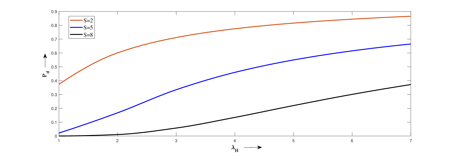
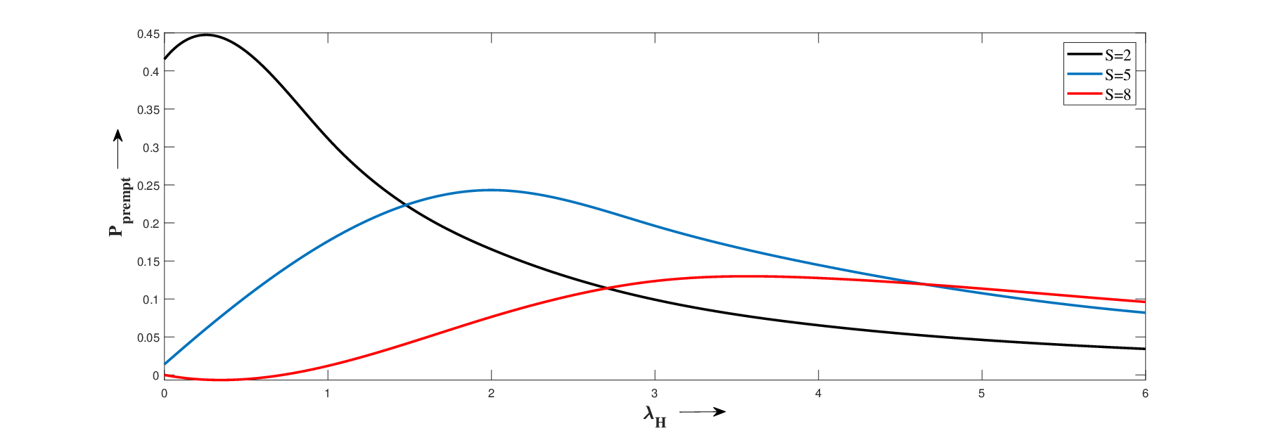
Figures 2(a) and 2(b) represent $P_{d}$ and $P_{preempt}$ as functions of total number of channels $S$ and $\lambda_{\mathcal{H}}$. It can be observed from Figure 2(a) that $P_{d}$ increases with respect to $\lambda_{\mathcal{H}}$ for a fixed value of $S$. Moreover, under the same value of $\lambda_{\mathcal{H}}$, $P_{d}$ decreases with respect to $S$. When handoff calls arrive frequently in the system, all the channels are most likely to be occupied by handoff calls and consequently extra handoff calls will be dropped. Therefore, the value of $P_{d}$ increases with increasing $\lambda_{\mathcal{H}}$. In this scenario, if the total channels are increased in the system, more handoff call will be able to obtain the service, as a result, $P_{d}$ decreases. Figure 2(b) exhibits the impact of $\lambda_{\mathcal{H}}$ and $S$ over $P_{preempt}$. It is seen from the graph that the values of $P_{preempt}$ for different $S$, first increase, and then decrease. The cause for this behavior of $P_{preempt}$ lies in the following explanation. When $\lambda_{\mathcal{H}}$ is relatively small, an arriving handoff call often finds at least one channel available, and consequently the ongoing service of a new call is not preempted by the arriving handoff call. As $\lambda_{\mathcal{H}}$ increases, the number of handoff calls also increase in the system. If an arriving handoff call finds all the channels occupied and at least one of them is serving a new call, the service of that new call will be preempted by the arriving handoff call. Hence, $P_{preempt}$ increases and reaches maximum at some value of $\lambda_{\mathcal{H}}$. Further, the decreasing behaviour of $P_{preempt}$ is explained by the fact that, with the increment in $\lambda_{\mathcal{H}}$, all the channels are occupied with handoff calls. Thus, the number of new calls in the service decreases and the probability that an arriving handoff call preempts the service of a new call decreases. These figures provide some advantageous results for the proposed model and these results are opted to formulate an optimization problem later on.

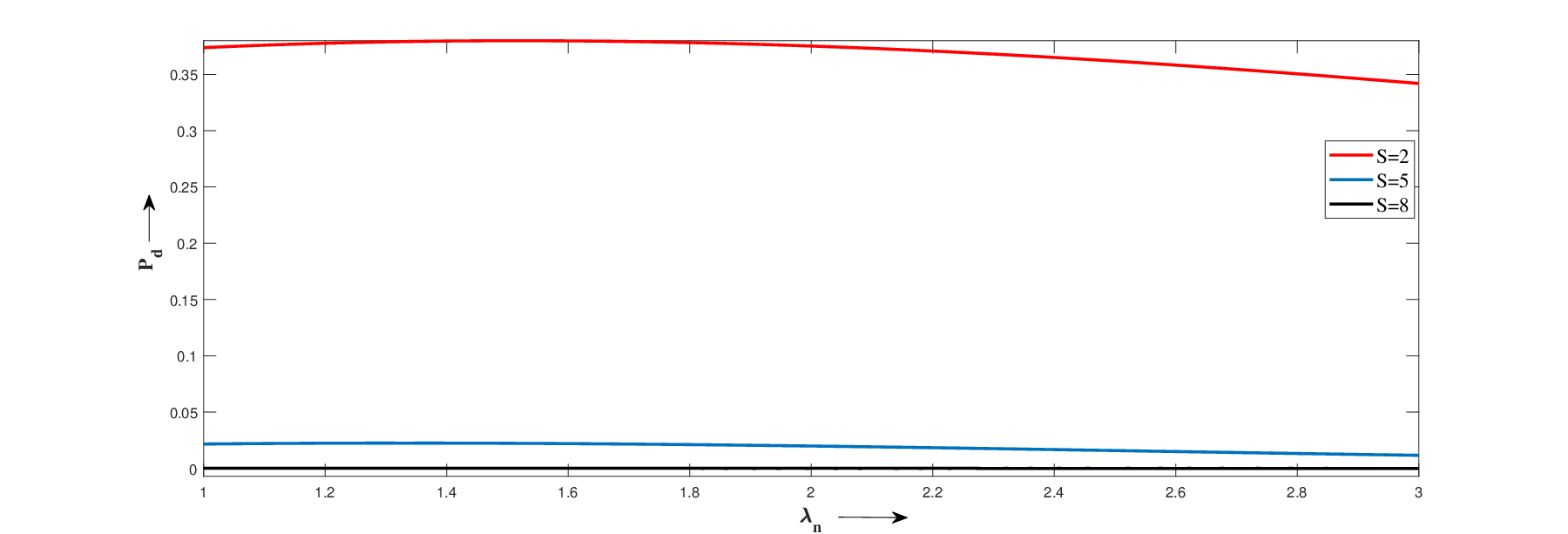
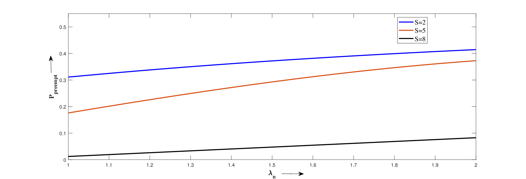
Figures 3(a) and 3(b) describe the behaviour of $P_{d}$ and $P_{preempt}$ corresponding to $\lambda_{\mathcal{N}}$ and $S$. The plot 3(a) exhibits that $P_{d}$ is less affected by an increment in $\lambda_{\mathcal{N}}$ but $P_{d}$ decreases with the increasing value of $S.$ Whereas, an obvious increasing behaviour of $P_{preempt}$ is observed from Figure 3(b) when $\lambda_{\mathcal{N}}$ increases. More interestingly, $P_{preempt}$ decreases when $S$ increases in the system. Such behaviour of $P_{preempt}$ can be explained as follows. When the number of new calls receiving service in the system is very less, the probability of preemption for new calls also decreases and as $\lambda_{\mathcal{N}}$ increases, $P_{preempt}$ also increases. Though, this probability can be reduced by increasing $S$ in the system.

Experiment 2: In this experiment, the impact of the service rate of handoff calls ($\mu_{\mathcal{H}}$) is shown over $P_{d}$ and $P_{preempt}$.

Figures 4(a) and 4(b) show the decreasing behaviour of $P_{d}$ and $P_{preempt}$ as $\mu_{\mathcal{H}}$ increases in the system. Further, it can also be observed from Figures 4(a) and 4(b) that, for the fixed value of $\mu_{\mathcal{H}}$, $P_{d}$ and $P_{preempt}$ decrease as $S$ increases. An intuitive explanation for this finding can easily be given as follows. As $\mu_{\mathcal{H}}$ increases, the calls are served with increasing rate, consequently the loss probabilities for both types of calls decrease. If $S$ is increased in the system, the chances for both types of calls to obtain the service also increase and consequently $P_{d}$ and $P_{preempt}$ decrease.

Experiment 3: The main purpose of this experiment is to observe the behaviour of intensity by which a retrial call is successfully connected to an available channel ($\theta_{r}^{succ}$) and the probability that a retrial call will exit the system without obtaining the service ($P_{leave}^{no-service}$) with respect to the retrial rate ($\theta$).

Figures 5(a) and 5(b) represent the behaviour of $\theta_{r}^{succ}$ and $P_{leave}^{no-service}$ with respect to $\theta$, respectively. It can be seen from the graphs when the value of $\theta$ increases, $\theta_{r}^{succ}$ increases. This impact can easily be explained as follows. When $\theta$ increases, the probability of a retrial call getting a connection also increases. For the fixed value of $\theta$, this probability is substantially greater for the large value of $S.$ The opposite impact of $\theta$ over $P_{leave}^{no-service}$ can be observed from Figure 5(b). When $\theta$ increases, the probability that a retrial call leaves the system without obtaining the service decreases. Moreover, decreasing behaviour of $P_{leave}^{no-service}$ is observed with respect to $S$ for the fixed value of $\theta$. When the number of available channels increases in the system, the probability for retrial call to obtain the service also increases. From 2(a) and 2(b), it can be observed that $\lambda_{\mathcal{H}}$ has vital impact over $P_{d}$ and $P_{preempt}$ when all other parameters of the system are fixed according to the system requirement. This observation is the main motivation for the formulation of the optimization problem illustrated in Section 6.

References

- [1] Artalejo, J.R., Dudin, A.N. and Klimenok, V.I., 2001. Stationary analysis of a retrial queue with preemptive repeated attempts. Operations Research Letters, 28(4), pp.173-180.
- [2] Baumann, H. and Sandmann, W., 2013. Computing stationary expectations in level-dependent QBD processes. Journal of Applied Probability, 50(1), pp.151-165.
- [3] Brandwajn, A. and Begin, T., 2017. Multi-server preemptive priority queue with general arrivals and service times. Performance Evaluation, 115, pp.150-164.
- [4] Bright, L. and Taylor, P.G., 1995. Calculating the equilibrium distribution in level dependent quasi-birth-and-death processes. Stochastic Models, 11(3), pp.497-525.
- [5] Chakravarthy, S.R., 2020. A Retrial Queueing Model with Thresholds and Phase Type Retrial times. Journal of Applied Mathematics & Informatics, 38(3-4), pp.351-373.
- [6] Chang, W., 1965. Preemptive priority queues. Operations research, 13(5), pp.820-827.
- [7] Dayar, T., 2012. Analyzing Markov chains using Kronecker products: theory and applications. Springer Science & Business Media.
- [8] Dharmaraja, S., Jindal, V. and Alfa, A.S., 2008. Phase-type models for cellular networks supporting voice, video and data traffic. Mathematical and computer modelling, 47(11-12), pp.1167-1180.
- [9] Drekic, S. and Stanford, D.A., 2001. Reducing delay in preemptive repeat priority queues. Operations Research, 49(1), pp.145-156.
- [10] Dudin, A., Kim, C., Dudin, S. and Dudina, O., 2015. Priority retrial queueing model operating in random environment with varying number and reservation of servers. Applied Mathematics and Computation, 269, pp.674-690.
- [11] Dudin, A.N., Lee, M.H., Dudina, O. and Lee, S.K., 2016. Analysis of priority retrial queue with many types of customers and servers reservation as a model of cognitive radio system. IEEE Transactions on Communications, 65(1), pp.186-199.
- [12] Eberhart, R. and Kennedy, J., 1995, November. Particle swarm optimization. In Proceedings of the IEEE international conference on neural networks, 4, pp. 1942-1948.
- [13] Fiems, D. and De Vuyst, S., 2018. From exhaustive vacation queues to preemptive priority queues with general interarrival times. International Journal of Applied Mathematics and Computer Science, 28(4), pp. 695-704.
- [14] He, Q.M., 1996. Queues with marked customers. Advances in Applied Probability, 28(2), pp.567-587.
- [15] He, Q.M., 2014. Fundamentals of matrix-analytic methods. New York: Springer.
- [16] He, Q.M. and Alfa, A.S., 1998. The queues with a last-come-first-served preemptive service discipline. Queueing systems, 29(2), pp.269-291.
- [17] He, Q.M. and Li, H., 2003. Stability conditions of the MMAP [K]/G [K]/1/LCFS preemptive repeat queue. Queueing systems, 44(2), pp.137-160.
- [18] Jain, V., Raj, R. & Dharmaraja, S., 2020. Numerical optimization of loss system with retrial phenomenon in cellular networks. International Journal of Operations Research, In Press.
- [19] Kim, J. and Kim, B., 2016. A survey of retrial queueing systems. Annals of Operations Research, 247(1), pp.3-36.
- [20] Kirkpatrick, S., Gelatt, C.D. and Vecchi, M.P., 1983. Optimization by simulated annealing. Science, 220(4598), pp.671-680.
- [21] Klimenok, V., Dudin, A. and Vishnevsky, V., 2020. Priority Multi-Server Queueing System with Heterogeneous Customers. Mathematics, 8(9), p.1501.
- [22] Krishnamoorthy, A., Babu, S. and Narayanan, V.C., 2008. MAP/(PH/PH)/c queue with self-generation of priorities and non-preemptive service. Stochastic Analysis and Applications, 26(6), pp.1250-1266.
- [23] Latouche, G. and Ramaswami, V., 1999. Introduction to matrix analytic methods in stochastic modeling. Society for Industrial and Applied Mathematics.
- [24] Machihara, F., 1995. A bridge between preemptive and non-preemptive queueing models. Performance Evaluation, 23(2), pp.93-106.
- [25] Neuts, M.F., 1994. Matrix-geometric solutions in stochastic models: an algorithmic approach. Courier Corporation.
- [26] Shin, Y.W. and Moon, D.H., 2011. Approximation of M/M/c retrial queue with PH-retrial times. European journal of operational research, 213(1), pp.205-209.
- [27] Sun, B., Lee, M.H., Dudin, A.N. and Dudin, S.A., 2014. MAP+ MAP//N/ Queueing System with Absolute Priority and Reservation of Servers. Mathematical Problems in Engineering.
- [28] Torczon, V. and Trosset, M.W., 1998, May. From evolutionary operation to parallel direct search: Pattern search algorithms for numerical optimization. In Computing Science and Statistics, pp. 396-401.