A Survey of Knowledge Graph Embedding and Their Applications

Shivani Choudhary Tarun Luthra Ashima Mittal Rajat Singh Affiliation: Indian Institute of Technology Delhi Affiliation: Hauz Khas, Delhi-110016, India Email: shivani@sire.iitd.ac.in, Email: {mcs202475,anz208486,csz208507}@cse.iitd.ac.in

Abstract

Knowledge Graph embedding provides a versatile technique for representing knowledge. These techniques can be used in a variety of applications such as completion of knowledge graph to predict missing information, recommender systems, question answering, query expansion, etc. The information embedded in Knowledge graph though being structured is challenging to consume in a real-world application. Knowledge graph embedding enables the real-world application to consume information to improve performance. Knowledge graph embedding is an active research area. Most of the embedding methods focus on structure-based information. Recent research has extended the boundary to include text-based information and image-based information in entity embedding. Efforts have been made to enhance the representation with context information. This paper introduces growth in the field of KG embedding from simple translation-based models to enrichment-based models. This paper includes the utility of the Knowledge graph in real-world applications.

1 Introduction

Knowledge graph(KG) has received a lot of traction in the recent past and led to much research in this area. Most of the research is focused on the generation of Knowledge graphs and consumption of the information enshrined in the Knowledge Graph. Some of the earlier works to create KG are YAGO(Suchanek et al. 2007), Freebase(Bollacker et al. 2008), DBpedia(Lehmann et al. 2012) and WikiData(Vrandečić and Krötzsch 2014). The evolution of the Knowledge Graph starts with the seminal paper from Berners-Lee (Berners-Lee et al. 2001). The knowledge graph has evolved in three phases. In the first phase, the Knowledge representation was brought to the level of Web standard. The core focus shifted to Data management, linked data, and its application in the second phase. In the third phase, the focus shifted on the real-world application (Bonatti et al. 2018). The real-world application ranges from Semantic parsing(Berant et al. 2013; Heck and Huang 2014), recommender system(Sun et al. 2020; Wang et al.), question answering(Saxena et al.), named entity disambiguation(Lin et al.), information extraction (Xiong and Callan; Xiong and Callan; Liu et al. 2018; Dietz et al. 2019) etc. The knowledge graph is a representation of structured relational information in the form of Entities and relations between them. It is a multi-relational graph where nodes are entities and edges are relations. Entities are real-world objects or abstract information. The representation entities and relations between them are represented as triple. For e.g. (New Delhi, IsCapitalOf, India) is an example of a triple. New Delhi and Delhi are entities and IsCapitalOf is relation. Though the representation looks scientific but consuming these in the real-world application is not an easy task. The consumption of information enshrined in the knowledge graph will be very easy if it can be converted to numerical representation. Knowledge graph embedding is a solution to incorporate the knowledge from the knowledge graph in a real-world application.
The motivation behind Knowledge graph embedding (Bordes et al.) is to preserve the structural information, i.e., the relation between entities, and represent it in some vector space. This makes it easier to manipulate the information. Most of the work in Knowledge graph embedding (KGE) is focused on generating a continuous vector representation for entities and relations and apply a relationship reasoning on the embedding. The relationship reasoning is supposed to optimize some scoring function to learn the embedding. Researchers have used different approaches to learn the embedding Path-based learning(Toutanova et al. 2016), Entity-based learning, textual-based learning, etc. A lot of work was focused were translation model (Bordes et al.) and semantic-based model(Bordes et al. 2014). The representation of the triple results in a lot of information lost because it fails to take ”textual information” into account. With the proposal of Graph attention network (Velicković et al. 2017) the representation of the entities has become more contextualized. In recent years, the proposal of multi-modal graph has extended the spectrum to a new level. In multi-modal knowledge graph, Knowledge graph can have multi-modal information like image and text etc. (Sun et al. 2020; Wei et al. 2019).
Previous work on survey has focused on the KG Embedding (Wang et al.), KG Embedding and application(Ji et al. 2020) , KG embedding with textual data (Lu et al. 2020), KG embedding based on the deep-learning (Wang et al. 2020). This work shall focus on the KG embedding from translation-based model, semantic-based model, embedding with enriched representation from textual data and multi-modal data and their application. In section 2, we shall provide the details of KGE; in section 3, we shall present the application area. In the summary section, we shall try to put emerging areas of research in KGE.

2 Knowledge Graph embedding

Knowledge Graph embedding is an approach to transform Knowledge Graphs (nodes, edges, and their feature vectors) into a low dimensional continuous vector space that preserves various graph structure, information, etc. These approaches are broadly classified into two groups: translation models and semantic matching models.

2.1 Translation Models

The translation-based model uses distance-based measures to generate the similarity score for a pair of entities and their relationships. The translation-based model aims to find a vector representation of entities with relation to the translation of the entities. It maps entities to a low-dimensional vector space.

2.1.1 TransE (Bordes et al. 2014)

The first model proposed was TransE. It is an energy based model. If a triple h, r, t holds then the vector representation h and r should be as close as possible. It can be graphically represented as Figure-1. Mathematically, it can be stated like $\textit{h}+\textit{r}\approx\textit{t}$ . The energy of a triple is d(h + r,t) for some similarity measure d. To learn the embedding, minimization of ranking based loss function over the training set.

\mathcal{L=\sum_{\textit{h,r,t}\in S}\sum_{\textit{$\hat{h}$,r,$\hat{t}$}\in\hat{S}}[\gamma+\textit{d(h+r),t}-\textit{d($\hat{h}$,r,$\hat{t}$)}]}

(1)

d(ĥ,r,t̂) represents the set of the corrupt triples. This loss function will be optimized so that the valid triples are ranked above the corrupt triples. This model fails in case of the one to many relation and many to many relation. To overcome this deficit new model TransH is proposed.

Refer to caption — Figure 1: The intuition of TransE model. Image credit Wang et al.

2.1.2 TransH Wang et al. 2014

It was proposed to address the limitations of TransE. This model enables an entity to have distributed representations based on their involvement in the relation. The representation of $h_{\bot}$ , $t_{\bot}$ are projected in a relation specific hyperplane. The relation between then is $d_{r}$ . As in the Figure-2, the vectors h and t are projected in the relation hyper-plane. The loss function and intuition remain similar to TransE.

2.1.3 TransR Lin et al. 2015

It proposes that an entity may have multiple attributes and various relations. Each relation may focus on different attributes of entities. TransR models entities and relation in different embedding space. It means that two different spaces: entity space and relation space are modelled. Each entity is mapped into relation space. The translation construct is applied on the projected representation in the relationship space. The Figure-3 presents the intuition behind TransR model.

To further refine the representation, a new model TransD was proposed by Ji et al. 2015. TransR captures the possibility of relations and their embedding from the relation space. But the TransD, extends it to the entity space as well. Here Entity-relation pair is considered as the first-class object.

2.1.4 RotatE Sun et al. 2019a

In knowledge graphs, often, the relation is symmetric/anti-symmetric, inversion and composition. e.g., ”Marriage” is a symmetric relation, ”My niece is my sister’s daughter” is a composition, etc. The models discussed above are not capable of predicting these relations. The model proposed here is based on the intuition that the relation from head to tail is modeled as rotation in a complex plane. It is motivated by Euler’s identity.

e^{\iota\theta}=\sin\theta+\iota\cos\theta

(2)

For a triplet (h,r,t), the relation among them can be represented as t = h $\circ$ r. Where h, r, t is the k-dimension embedding of the head, relation and tail, restricting the $|{r_{i}}|$ = 1. It means we are in the unit circle and $\circ$ represents element wise product. For each dimension $t_{i}=r_{i}h_{i}$ subjected to constraint $|{r_{i}}|$ = 1. Under these condition the relationship is symmetric $\iff$ for all the values of i, $e^{0/\iota\theta}=\pm 1$ , The relationship is inverse $\iff$ $r_{j}=\bar{r}_{i}$ , i.e. both are the complex conjugate. Two relations are composite $\iff$ $r_{j}=r_{i}\circ r_{k}$ . It means the relation $r_{j}$ can be obtained by a combined rotation of $r_{i}$ and $r_{k}$ , $\theta_{j}=\theta_{i}+\theta_{k}$ . The scoring function measures the angular distance.

d_{r}(h,t)=\left\|h\circ r-t\right\|

(3)

The Figure-4 shows the comparison of RotaE and TransE.

2.1.5 HakE Zhang et al. 2019

The approaches we have discussed so far fails to capture the semantic hierarchies. In HakE, the authors have proposed to model the hierarchy in the entities as concentric circles in polar coordinate. The entity with smaller radius belongs to higher up in the hierarchy. The angle between them represents the variation in the meaning. To represent a point on the circle, we should have $(r,\theta)$ . Similarly, this model has two components, one to map the modulus and the other one to map the angle. The modulus part considers the depth of the tree as moduli. Let $h_{m},t_{m}$ and $r_{m}$ are the representation in modulus space then $h_{m}\circ r_{m}=t_{m}$ , where $h_{m},t_{m}$ is a k-dim vector. The distance function is similar to RotatE with modification to consider only modulo part.

d_{r,m}(h_{m},t_{m})=\left\|h_{m}\circ r_{m}-t_{m}\right\|_{2}

(4)

Similarly, the phase part can be formulated as $(h_{p}+r_{p})mod2\pi=t_{p}$ where $h_{p},r_{p},t_{p}\in[0,2\pi)^{k}$ . The distance function is

d_{r,p}(h_{p},t_{p})=\left\|\sin((h_{p}\circ r_{p}-t_{p})/2)\right\|_{1}

(5)

By combining both the part, an entity can be mapped in the polar coordinate space.

2.2 Semantic Matching Models

Semantic Matching is one of the core tasks in Natural Language Processing. As we have seen that Translational Distance Models use distance-based scoring functions to calculate the similarity between the different entities and relations thus build the embedding accordingly. On the other hand, Semantic Matching Models use similarity-based scoring function. There are several Knowledge Graph Embedding algorithms comes under this model. Some of the algorithms are described below.

2.2.1 RESCAL Nickel et al. 2011

RESCAL follows Statistical Relational Learning Approach which is based on a Tensor Factorization model that takes the inherent structure of relational data into account. A TensorKolda and Bader 2009 is a multidimensional array. More formally we can say that a first order Tensor is a vector, second order Tensor is a matrix and, Tensor with more than two order is called as higher order Tensor. Tensor Factorization is expressing a Tensor as a sequence of elementary operations acting on other, often a simpler Tensors. Statistical Relational Learning inherits from Probability Theory and Statistics to address uncertainty and complexity of relational structures.
Nickel et al. 2011 models the Knowledge Graph triplet of the form (head, relation, tail) into three-way tensor, $\mathcal{X}$ as shown in Figure 5.

In $\mathcal{X}$ , two modes holds the concatenated entities (head and tail), and the third mode holds relation (relation). A Tensor entity $\mathcal{X}_{ijk}$ = 1 denotes that there exist a relation and if $\mathcal{X}_{ijk}$ = 0 denotes that there is unknown relation. It is assumed that data is given as n * n * m Tensor. Where n is the number of entities and m is the number of relations. RESCAL ”explains triples via pairwise interaction of latent features”. It performs the rank-r factorization on each slice of $\mathcal{X}$ (relational data) and the score of a fact (head, relation, tail ) is given by the following bi-linear function.

f_{r}(h,t)=\textbf{h}^{T}\textbf{M}_{r}\textbf{t}=\sum_{i=0}^{d-1}\sum_{j=0}^{d-1}[\textbf{M}_{r}]_{ij}.[\textbf{h}]_{i}.[\textbf{t}]_{j}

where h,t $\in$ $\mathbb{R}^{d}$ are vector representation of entities, and $M_{r}$ $\in$ $\mathbb{R}^{d*d}$ is a matrix representation of $r^{th}$ relation. Thus from this equation we are able to calculating the score of the triple using the weighted sum of all the pairwise interactions between the latent features of the entities $h$ and $t$ as shown in the Figure 6.

This method require $O(d^{2})$ parameters per relation and the space complexity of $O(nd+md^{2})$ where n is the number of entities and m is the number of relations.

2.2.2 TATEC García-Durán et al. 2014

TATEC stands for Two And Three-way Embeddings Combination. The main disadvantage of RESCAL is that it is a Three-way model which performs fairly good for relationships which occur frequently but it performs poor for the rare relationships and leads to major over-fitting. The issue of major over-fitting for rare relationships can be controlled by regularizing or reducing the expressivity of the model and former method is not feasible. The second method of reducing the expressivity is Two-way interaction which is implemented in TransE and SME. Two-way interaction approaches overperform the Three-way approaches on many datasets from which we can conclude that Two-way interactions are more efficient for the datasets and specially for those datasets which have more rare relationships. But the problem with the two-way interaction is that they are limited and are not able to represent all kind of relations with entities.
TATEC is a latent factor model which is capable of incorporating the high capacity Three-way model with well-controlled two-way interactions and take the advantage of both of them. Since two-way and three-way models do not use the the same kind of data pattern and do not encode the same kind of information in the embedding. So, in TATEC during first stage they used two different embeddings and then combined and fine-tuned them in the later stage. The scoring function of TATEC is given by $f_{r}(h,t)=f_{r}^{1}(h,t)+f_{r}^{2}(h,t)$ which is a linear combination of bi-gram and tri-gram terms, where $f_{r}^{1}(h,t)$ is a two-way interaction score and $f_{r}^{2}(h,t)$ is a three-way interaction score. These can be calculates as follows:
1) Two-way interactions terms can be given by:

f_{r}^{1}(h,t)=\textbf{h}^{T}\textbf{r}+\textbf{t}^{T}\textbf{r}+\textbf{h}^{T}\textbf{D}\textbf{t}

where D is the diagonal matrix shared across all the different relations and does not depend on input triple and r $\in$ $\mathbb{R}^{d}$ is a vector that depends on relationships.
2) Three-way interactions terms can be given by:

f_{r}^{2}(h,t)=\textbf{h}^{T}\textbf{M}_{r}\textbf{t}

The final scoring function of TATEC is given by

f_{r}(h,t)=\textbf{h}^{T}\textbf{M}_{r}\textbf{t}+\textbf{h}^{T}\textbf{r}+\textbf{t}^{T}\textbf{r}+\textbf{h}^{T}\textbf{D}\textbf{t}

Authors of García-Durán et al. 2014 compared this model to the other existing models such as RESCAL Nickel et al. 2011, TransE (Bordes et al.), LFM, SE and, SME for link prediction on FB15k dataset and as a result TATEC performs better than all other available models as shown in Figure 7.

Time complexity and the space complexity of TATEC is same as RESCAL as TATEC extends RESCAL. The time complexity of TATEC is $O(d^{2})$ parameters per relation and the space complexity of $O(nd+md^{2})$ where n is the number of entities and m is the number of relations.

2.2.3 DistMult Yang et al. 2014

This model compares with the NTN neural model, TransE and bi-linear models like RESCAL. The problem with NTN is that it is the most expensive model it incorporate both linear and bilinear relation operations. Similarly TransE parameterizes the linear operations with one dimensional vectors. DistMult is a simplified RESCAL, which uses the basic bilinear scoring function.

f_{r}(h,t)=\textbf{h}^{T}\textbf{M}_{r}\textbf{t}

These bilinear formulations are combined with different forms of regularization to make different models. In DistMult authors considered a simpler approach where they reduced the number of parameters by imposing restrictions on $M_{r}$ to be a diagonal matrix. This results in a simpler model and this model enjoys the same scalable properties of TransE as well as it achieves better performance over TransE. Thus the final scoring function is given as

f_{r}(h,t)=\textbf{h}^{T}diag(\textbf{r})\textbf{t}=\sum_{i=0}^{d-1}[\textbf{r}]_{i}.[\textbf{h}]_{i}.[\textbf{t}]_{i}

where for each relation r, r $\in\mathbb{R}^{d}$ is a vector that depends on relationships.

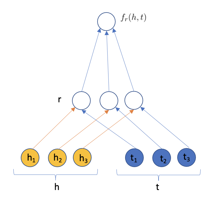
Time complexity and the space complexity of DistMult is more efficient as compared to RESCAL or TATEC. The time complexity of DistMult is $O(d)$ parameters per relation and the space complexity of $O(nd+md)$ where n is the number of entities and m is the number of relations. Due to its over-simplified mature of the model, this model is not enough powerful for the use in case of general Knowledge Graphs because it is only able to work efficiently with symmetric relations.

2.2.4 HolE Nickel et al. 2016b

HolE stands for Holographic Embedding. HolE tried to overcome the problem of Tensor Product used in RESCAL by using circular correlation. Tensor product uses pairwise multiplicative interactions between feature vectors which results in increase in dimensionality of the representation i.e., $\mathbb{R}^{d^{2}}$ thus increase the computational demand.

\textbf{h}\circ\textbf{t}=\textbf{h}\otimes\textbf{t}\in\mathbb{R}^{d^{2}}

Where a,b $\in\mathbb{R}^{d}$ are entity embeddings. Tensor products are very rich in capturing the interactions but are computational intensive. On the other hand HolE use Circular Correlation which can be seen as compression of the Tensor Product. The main advantage of Circular Correlation over Tensor Product is that it won’t increase the dimensionality of the representation.

\textbf{h}\circ\textbf{t}=\textbf{h}*\textbf{t}\in\mathbb{R}^{d}

Where * : $\mathbb{R}^{d}\times\mathbb{R}^{d}\rightarrow\mathbb{R}^{d}$ denotes the circular correlation.

[\textbf{h}*\textbf{t}]_{i}=\sum_{k=0}^{d-1}[\textbf{h}_{k}].\textbf{t}_{(k+i)mod(d)}

The final score of the fact in HolE is given by matching the compositional vector ( $\textbf{h}*\textbf{t}$ ) with the relational representation,i.e.,

f_{r}(h,t)=\textbf{r}^{T}(\textbf{h}*\textbf{t})=\sum_{i=0}^{d-1}[\textbf{r}]_{i}\sum_{k=0}^{d-1}[\textbf{h}]_{k}.[\textbf{t}]_{(k+i)mod(d)}

So HolE is more efficient as compared to RESCAL or TransE. HolE take $O(dlogd)$ parameters per relation and the space complexity of $O(nd+md)$ where n is the number of entities and m is the number of relations. Another advantage of HolE is that Circular Correlation is not commutative ( $\textbf{h}*\textbf{t}\neq\textbf{t}*\textbf{h}$ ) thus HolE is able to model asymmetric relations (directed graphs) with compositional representations which is not possible in RESCAL.

2.2.5 ComplExTrouillon et al. 2016

Knowledge graphs represent the relation between entities. The entities may be termed as subjects and objects respectively of a given relation. However not all relations may be present in a given KG. One of the application of KG is the ability to predict missing relations or entities.
Dot product of vector embedding of KG triplets is being successfully used for symmetric, reflexive, anti-reflexive and even transitive relations (Bouchard et al. 2015) however it can’t be used for anti-symmetric relations. For example the relation capitalOf(New Delhi, India) is not symmetric since we cannot interchange subject and object entity in this relation therefore we need to have different embedding for an entity as subject and as object which increases the number of parameters.
Complex embedding facilitates joint learning of subject and object entities while preserving the asymmetry of the relation. It uses Hermitian dot product of embedding of subject entities and object entities. The Eigen Vector decomposition is used to identify a low rank diagonal matrix W such that there exists X = Re( $EWE^{T}$ ) such that X has same sign pattern as Y. The low rank diagonal matrix W is then used to predict missing relations by applying Re( $e_{s}^{T}W\bar{e}_{o}$ ).

2.2.6 ANALOGYLiu et al. 2017

ANALOGY is based on a multiplicative model where the relation (s,r,o) is scored by multiplying the vector representations of of subject (s), relation (r) and object (o). The relation present in the knowledge graph are expected to have higher score i.e. $\phi(s,r,0)$ = $e_{s}^{T}W_{r}e_{o}$ will be high if the triplet (s,r,o) exists.
An example of analogy may be branch:tree::petal:leaf, in such an analogy, the relation $W_{r}$ ”is part of” may be used to predict the missing entity from the analogy. The foundation of ANALOGY model is the linear maps of matrix representation of relations from the triplets present in the KG. Basically, the model uses the fact that there can be multiple paths to arrive at the entity from a given entity through a linear map of relations $W_{r1},W_{r2},W_{r3}$ and so on, and application of such relations in any sequence will give the same result. Hence such linear maps may be used to predict entities missing from the knowledge graph.
For example Let’s consider the entities teacher (t), school (s), professor (p) and college (c). We have two relations in this set up: teachesAt (t,s) & teachesAt(p,c) and juniorOf(t,p) & juniorOf(s,c) therefore the relation between teacher and college is teachesAt*juniorOf = juniorOf*teachesAt. However such linear maps are feasible only if the commutative property holds for such relations. ANALOGY uses such linear maps to predict entities.

2.3 Enrichment based embedding

In the recent times, new emerging research areas are focusing on contextualized embedding. Under this, the entity under the consideration is enriched information from the neighbourhood information. A few notable approaches are Graph attention network (GAT) (Velicković et al. 2017) based information enrichment. Two methods based on the KGAT (Wei et al. 2019), MMGAT (Sun et al. 2020) has proposed models to embed contextual information for an entity. Under MMGAT, they proposed model to combine the embedding from multi-modal data with an attention framework, as adopted from GAT’s attention framework. Both the frameworks, were using translation model to learn the representation after the enrichment. The new emerging research areas are try to learn the structural information as well as path based information, multi-modal data. There are other research areas in the embedding are: Text-enhanced embedding, Logic-enhanced embedding, Image-enhanced embedding (Bianchi et al. 2020) etc.

3 Applications of Knowledge graph embedding

There are many applications of KG embedding learning methods. This section explores three of them namely- link prediction, triplet classification and recommender systems.

The first two are In-KG applications, which are conducted within the scope of the KG. The last is an example of Out-of-KG applications that scale to broader domains (Wang et al. 2017).

3.1 Link Prediction

The set of edges in a knowledge graph is a subset of Entities $\times$ Relations $\times$ Entities. The link prediction task focuses on finding an entity that can be represented as a fact (edge) together with a given relation and entity i.e., (entity, relation, ?) or (?, relation, entity) where ? refers to the missing entity. For e.g. (New Delhi, isCapitalOf, ?) or (?, isCapitalOf, India). Link prediction is a way of Knowledge graph augmentation (Paulheim 2017). It deduces missing information from the knowledge graph itself.

The datasets for LP are constructed by sampling from the original knowledge graph. Then, the links removed can be used in validation set or the test set (Bordes et al. 2013; Dettmers et al. 2018). The structure of such graphs play a vital role for improving the results, multiple source entities making learning effective and multiple destination entities making learning difficult (Rossi et al. 2021).

The LP models assigns a score to the triplet corresponding to each possible entity to fill the question mark (?). The triplets are then ranked by a function and entity corresponding to the lowest rank is predicted. If the predicted facts in the ranked predictions are already present in the Knowledge graph, they may or may not be excluded while calculating the ranks called raw and filtered rankings respectively (Bordes et al. 2013). For e.g. if the training knowledge graph contains the fact that (Arjuna, isSonOf, Kunti), and the test query is (?, isSonOf, Kunti). The target answer is (Yudhishtra, isSonOf, Kunti) and the system ranks (Arjuna, isSonOf, Kunti) and then (Yudhishtra, isSonOf, Kunti). The raw ranking of the triplet (Yudhishtra, isSonOf, Kunti) will be two and filtered ranking will be one.

There are several tie breaking policies that are used by the ranking system. Assigning the minimum or the maximum rank, or a random or the average rank to the targeted entity (Rossi et al. 2021).

The ranks obtained are used to compute metrics such as Mean Rank (average of all the ranks), Mean Reciprocal Rank (average of the inverse of ranks), or Hits@M (proportion of ranks $\leq$ M).

3.2 Triple Classification

Triple Classification is the problem of identifying whether a given triple is correct. It aims to give a yes or no answer to questions such as is New Delhi capital of India? which can be written in the form of a triple (New Delhi, isCapitalOf, India) (Socher et al. 2013).

A scoring function is used to calculate score of a triple similar to the link prediction. If the score is greater than a certain threshold, then it is considered a fact else a wrong triple (Wang et al. 2017).

Both the classical methods, such as micro and macro averaging, and ranking methods such as Mean Rank are used as evaluation metrics (Guo et al. 2016).

3.3 Recommender Systems

Recommender system (RS) assists the user in an environment where multiple options are available by providing a certain ordering of choices that the recommendation algorithm infers. This inference can be based on the similarity of the choices and behaviour pattern of different users. This type of recommendation methods falls into the domain of collaborative filtering methods (Adomavicius and Tuzhilin 2005).

The CF methods suffer from problems of Data sparsity and cold start. Data sparsity arises from the fact that only a small proportion of items are rated by the users and most options have only limited feedback from the users. Cold start problem is the problem of having no historical data about the new users and options. To deal with these problems different types of side information about a user and item are utilized by the RS (Sun et al. 2019b).

KG is utilised for side information in CF. It acts as a heterogeneous graph that represent entities as nodes and relation as edges. The KG connects various entities via latent relationships and also provide explainability in recommendations (Wang et al. 2018).

The KG embedding based methods for RS use two modules - Graph embedding and Recommendation Module. The way that these modules are coupled lead to categorization of embedding based methods in a). two stage learning methods, b). joint learning method and c). multi task learning method(Guo et al. 2020).

Two stage learning methods first uses graph embedding module to obtain the embeddings using various KG algorithms and then use recommendation module to infer. The advantages of this method lies in its simplicity and scalability but since the two modules are loosely coupled the embeddings might not be suitable for recommendation tasks.

Joint learning methods train both the modules in an end to end fashion. Thus, recommendation module guides the training in graph embedding layer.

Multi task learning method train the recommendation module with the guidance of KG related task such as KG completion. The primary intuition behind this method is that the bipartite graph of user and item in recommendation task share structures with the corresponding KG entities.

4 Summary

Knowledge graphs provide an effective way of presenting real-world relationships. As a result Knowledge graphs have an inherent advantage w.r.t serving the information need. KG in itself is a growing area of research. KG embedding is a technique to represent all the components of the KG in vector form. These vectors represent the latent properties of the components of the graph. Various models for embedding methods are based on different combinations of vector algebra which present an interesting area of research. In this work, we have surveyed the embedding methods that started this active area of research, state-of-art models and the new frontiers which are being explored in the KG embedding.
The KG embedding methods progressed from translation-based models which are based on vector addition. In this work, we have presented how translation-based models improved over time to overcome shortcomings of the earlier models. While translation-based models used vector addition, semantic models can be clubbed together as multiplicative models. We have included the transition from basic semantic models to the more advanced semantic models which may be used to explain different types of real world relationships such as symmetric, anti-symmetric,inverse or composition.
New research areas have broaden the scope from structural embedding to more contextual embedding by encoding additional information in the learned representation. The latest area of research in this field is enrichment based embedding models. In this work, we have introduced those briefly.
Vector space representation has paved a way to use the information from Knowledge graph directly into the real world application. In this work, we have described a few real world applications of KG embedding such as link prediction, triple classification and recommender systems.

References

Adomavicius and Tuzhilin (2005) Gediminas Adomavicius and Alexander Tuzhilin. 2005. Toward the next generation of recommender systems: A survey of the state-of-the-art and possible extensions. IEEE transactions on knowledge and data engineering, 17(6):734–749.
Berant et al. (2013) Jonathan Berant, Andrew Chou, Roy Frostig, and Percy Liang. 2013. Semantic Parsing on Freebase from Question-Answer Pairs. Technical report.
Berners-Lee et al. (2001) Tim Berners-Lee, James Hendler, and Ora Lassila. 2001. The Semantic Web A new form of Web content that is meaningful to computers will unleash a revolution of new possibilities. Sci. Am., 284(5):1–5.
Bianchi et al. (2020) F. Bianchi, G. Rossiello, Luca Costabello, M. Palmonari, and Pasquale Minervini. 2020. Knowledge graph embeddings and explainable ai. ArXiv, abs/2004.14843.
Bollacker et al. (2008) Kurt Bollacker, Colin Evans, Praveen Paritosh, Tim Sturge, and Jamie Taylor. 2008. Freebase: A collaboratively created graph database for structuring human knowledge. In Proc. ACM SIGMOD Int. Conf. Manag. Data, pages 1247–1249, New York, New York, USA. ACM Press.
Bonatti et al. (2018) P. Bonatti, S. Decker, A. Polleres, and V. Presutti. 2018. Knowledge graphs: New directions for knowledge representation on the semantic web (dagstuhl seminar 18371). Dagstuhl Reports, 8:29–111.
Bordes et al. (2014) Antoine Bordes, Xavier Glorot, Jason Weston, and Yoshua Bengio. 2014. A semantic matching energy function for learning with multi-relational data: Application to word-sense disambiguation. Mach. Learn., 94(2):233–259.
(8) Antoine Bordes, Nicolas Usunier, Alberto Garcia-Durán, Jason Weston, and Oksana Yakhnenko. Translating Embeddings for Modeling Multi-relational Data. Technical report.
Bordes et al. (2013) Antoine Bordes, Nicolas Usunier, Alberto Garcia-Duran, Jason Weston, and Oksana Yakhnenko. 2013. Translating embeddings for modeling multi-relational data. In Neural Information Processing Systems (NIPS), pages 1–9.
Bouchard et al. (2015) Guillaume Bouchard, Sameer Singh, and Théo Trouillon. 2015. On approximate reasoning capabilities of low-rank vector spaces.
Dettmers et al. (2018) Tim Dettmers, Pasquale Minervini, Pontus Stenetorp, and Sebastian Riedel. 2018. Convolutional 2d knowledge graph embeddings. In Proceedings of the AAAI Conference on Artificial Intelligence, volume 32.
Dietz et al. (2019) Laura Dietz, Chenyan Xiong, Jeff Dalton, and Edgar Meij. 2019. Special issue on knowledge graphs and semantics in text analysis and retrieval. Inf. Retr. J., 22(3-4):229–231.
García-Durán et al. (2014) Alberto García-Durán, Antoine Bordes, and Nicolas Usunier. 2014. Effective blending of two and three-way interactions for modeling multi-relational data. In Machine Learning and Knowledge Discovery in Databases, pages 434–449, Berlin, Heidelberg. Springer Berlin Heidelberg.
Guo et al. (2020) Q. Guo, F. Zhuang, C. Qin, H. Zhu, X. Xie, H. Xiong, and Q. He. 2020. A survey on knowledge graph-based recommender systems. IEEE Transactions on Knowledge and Data Engineering, pages 1–1.
Guo et al. (2016) Shu Guo, Quan Wang, Lihong Wang, Bin Wang, and Li Guo. 2016. Jointly embedding knowledge graphs and logical rules. In Proceedings of the 2016 conference on empirical methods in natural language processing, pages 192–202.
Heck and Huang (2014) Larry Heck and Hongzhao Huang. 2014. Deep learning of knowledge graph embeddings for semantic parsing of Twitter dialogs. In 2014 IEEE Glob. Conf. Signal Inf. Process. Glob. 2014, pages 597–601. Institute of Electrical and Electronics Engineers Inc.
Ji et al. (2015) Guoliang Ji, Shizhu He, Liheng Xu, Kang Liu, and Jun Zhao. 2015. Knowledge graph embedding via dynamic mapping matrix. In Proceedings of the 53rd Annual Meeting of the Association for Computational Linguistics and the 7th International Joint Conference on Natural Language Processing (Volume 1: Long Papers), pages 687–696, Beijing, China. Association for Computational Linguistics.
Ji et al. (2020) Shaoxiong Ji, Shirui Pan, Erik Cambria, Pekka Marttinen, and Philip S. Yu. 2020. A survey on knowledge graphs: Representation, acquisition and applications. arXiv, pages 1–27.
Kolda and Bader (2009) Tamara G Kolda and Brett W Bader. 2009. Tensor decompositions and applications. SIAM review, 51(3):455–500.
Lehmann et al. (2012) Jens Lehmann, Robert Isele, Max Jakob, Anja Jentzsch, Dimitris Kontokostas, Pablo N Mendes, Sebastian Hellmann, Mohamed Morsey, Patrick Van Kleef, Sören Auer, and Christian Bizer. 2012. DBpedia-A Large-scale, Multilingual Knowledge Base Extracted from Wikipedia. Technical report.
(21) Brian Lin, Shane Ong, Cory Williams, Yun Bin, and Matteo Zhang. Named Entity Disambiguation with Knowledge Graphs. Technical report.
Lin et al. (2015) Yankai Lin, Zhiyuan Liu, Maosong Sun, Yang Liu, and Xuan Zhu. 2015. Learning entity and relation embeddings for knowledge graph completion. In Proceedings of the Twenty-Ninth AAAI Conference on Artificial Intelligence, AAAI’15, page 2181–2187. AAAI Press.
Liu et al. (2017) Hanxiao Liu, Yuexin Wu, and Yiming Yang. 2017. Analogical inference for multi-relational embeddings.
Liu et al. (2018) Zhenghao Liu, Chenyan Xiong, Maosong Sun, and Zhiyuan Liu. 2018. Entity-duet neural ranking: Understanding the role of knowledge graph semantics in neural information retrieval. ACL 2018 - 56th Annu. Meet. Assoc. Comput. Linguist. Proc. Conf. (Long Pap., 1:2395–2405.
Lu et al. (2020) Fengyuan Lu, Peijin Cong, and Xinli Huang. 2020. Utilizing Textual Information in Knowledge Graph Embedding: A Survey of Methods and Applications. IEEE Access, 8:92072–92088.
Nickel et al. (2016a) Maximilian Nickel, Kevin Murphy, Volker Tresp, and Evgeniy Gabrilovich. 2016a. A review of relational machine learning for knowledge graphs. Proceedings of the IEEE, 104(1):11–33.
Nickel et al. (2016b) Maximilian Nickel, Lorenzo Rosasco, and Tomaso Poggio. 2016b. Holographic embeddings of knowledge graphs. In Proceedings of the AAAI Conference on Artificial Intelligence, volume 30.
Nickel et al. (2011) Maximilian Nickel, Volker Tresp, and Hans-Peter Kriegel. 2011. A three-way model for collective learning on multi-relational data. In Icml.
Paulheim (2017) Heiko Paulheim. 2017. Knowledge graph refinement: A survey of approaches and evaluation methods. Semantic web, 8(3):489–508.
Rossi et al. (2021) Andrea Rossi, Denilson Barbosa, Donatella Firmani, Antonio Matinata, and Paolo Merialdo. 2021. Knowledge graph embedding for link prediction. ACM Transactions on Knowledge Discovery from Data, 15(2):1–49.
(31) Apoorv Saxena, Aditay Tripathi, and Partha Talukdar. Improving Multi-hop Question Answering over Knowledge Graphs using Knowledge Base Embeddings. Technical report.
Socher et al. (2013) Richard Socher, Danqi Chen, Christopher D Manning, and Andrew Ng. 2013. Reasoning with neural tensor networks for knowledge base completion. In Advances in neural information processing systems, pages 926–934. Citeseer.
Suchanek et al. (2007) Fabian M. Suchanek, Gjergji Kasneci, and Gerhard Weikum. 2007. Yago: A core of semantic knowledge. In 16th Int. World Wide Web Conf. WWW2007, pages 697–706.
Sun et al. (2020) Rui Sun, Xuezhi Cao, Yan Zhao, Junchen Wan, Kun Zhou, Fuzheng Zhang, Zhongyuan Wang, and Kai Zheng. 2020. Multi-modal Knowl-edge Graphs for Recommender Systems.
Sun et al. (2019a) Zhiqing Sun, Zhi-Hong Deng, Jian-Yun Nie, and Jian Tang. 2019a. Rotate: Knowledge graph embedding by relational rotation in complex space. CoRR, abs/1902.10197.
Sun et al. (2019b) Zhu Sun, Qing Guo, Jie Yang, Hui Fang, Guibing Guo, Jie Zhang, and Robin Burke. 2019b. Research commentary on recommendations with side information: A survey and research directions. Electronic Commerce Research and Applications, 37:100879.
Toutanova et al. (2016) Kristina Toutanova, Xi Victoria Lin, Wen Tau Yih, Hoifung Poon, and Chris Quirk. 2016. Compositional learning of embeddings for relation paths in knowledge bases and text. 54th Annu. Meet. Assoc. Comput. Linguist. ACL 2016 - Long Pap., 3:1434–1444.
Trouillon et al. (2016) Théo Trouillon, Johannes Welbl, Sebastian Riedel, Éric Gaussier, and Guillaume Bouchard. 2016. Complex embeddings for simple link prediction.
Velicković et al. (2017) Petar Velicković, Guillem Cucurull, Arantxa Casanova, Adriana Romero, Pietro Liò, and Yoshua Bengio. 2017. Graph attention networks. arXiv, pages 1–12.
Vrandečić and Krötzsch (2014) Denny Vrandečić and Markus Krötzsch. 2014. Wikidata: A free collaborative knowledgebase. Commun. ACM, 57(10):78–85.
Wang et al. (2018) Hongwei Wang, Fuzheng Zhang, Jialin Wang, Miao Zhao, Wenjie Li, Xing Xie, and Minyi Guo. 2018. Ripplenet. Proceedings of the 27th ACM International Conference on Information and Knowledge Management.
Wang et al. (2017) Quan Wang, Zhendong Mao, Bin Wang, and Li Guo. 2017. Knowledge graph embedding: A survey of approaches and applications. IEEE Trans. Knowl. Data Eng., 29(12):2724–2743.
Wang et al. (2020) Shirui Wang, Wenan Zhou, and Chao Jiang. 2020. A survey of word embeddings based on deep learning. Computing, 102(3):717–740.
(44) Xiang Wang, Xiangnan He, Yixin Cao, Meng Liu, and Tat-Seng Chua. KGAT: Knowledge Graph Attention Network for Recommendation.
Wang et al. (2014) Zhen Wang, J. Zhang, Jianlin Feng, and Z. Chen. 2014. Knowledge graph embedding by translating on hyperplanes. In AAAI.
Wei et al. (2019) Yinwei Wei, Xiangnan He, Xiang Wang, Richang Hong, Liqiang Nie, and Tat Seng Chua. 2019. MMGCN: Multi-modal graph convolution network for personalized recommendation of micro-video. MM 2019 - Proc. 27th ACM Int. Conf. Multimed., pages 1437–1445.
(47) Chenyan Xiong and Jamie Callan. Query Expansion with Freebase.
Yang et al. (2014) Bishan Yang, Wen tau Yih, Xiaodong He, Jianfeng Gao, and Li Deng. 2014. Embedding entities and relations for learning and inference in knowledge bases.
Zhang et al. (2019) Zhanqiu Zhang, Jianyu Cai, Yongdong Zhang, and Jie Wang. 2019. Learning hierarchy-aware knowledge graph embeddings for link prediction. CoRR, abs/1911.09419.