The -relaxed area of the graph of the vortex map
Abstract
We compute the value of the -relaxed area of the graph of the map , , , for all values of . Interestingly, for in a certain range, in particular not too large, a Plateau-type problem, having as solution a sort of catenoid constrained to contain a segment, has to be solved.
Key words: Relaxation, Cartesian currents, area functional, minimal surfaces, Plateau problem.
AMS (MOS) subject classification: 49Q15, 49Q20, 49J45, 58E12.
1 Introduction
Determining the domain and the expression of the relaxed area functional for graphs of nonsmooth maps in codimension greater than is a challenging problem whose solution is far from being reached. Given a bounded open set and a map of class , the area of the graph of over is given by the classical formula
| (1.1) |
where is the vector whose entries are the determinants of the minors of the gradient of of all orders11 1 By convention, the determinant of order is . , . Classical methods of relaxation suggest to consider the functional defined, for any , as
| (1.2) |
and called (sequential) relaxed area functional. The infimum is computed over all sequences of maps approaching in . The results of Acerbi and Dal Maso [1] show that extends and is -lower-semicontinuous. This procedure of relaxation, besides extending the notion of graph’s area to non-smooth maps, is needed also because is not -lower-semicontinuous22 2 When , there are sequences , with , weakly converging in to a smooth map for which , where is defined as for -maps in (1.1), with the determinant of intended in the almost everywhere pointwise sense; see [4, Counterexample 7.4] and [1]. This counterexample must be slightly modified, considering for , with satisfying , in order to get the strict inequality above. , in contrast with similar polyconvex functionals that enjoy a growth condition of the form for some , and suitable (see, e.g., [26, 11, 17]).
When it is possible to characterize the domain of and its expression [12]: is finite if and only if , in which case
| (1.3) |
and representing the absolutely continuous and singular parts of the distributional gradient of . Formula (1.3) is a basic example of non-parametric variational integral that is a measure when considered as a function of [20], and is crucial, among others, in the study of capillarity problems [16], and in the analysis of the Cartesian Plateau problem [19]. The case (referred here to as the case of codimension greater than ) is much more involved. Again, one of its main motivations is the study of the Cartesian Plateau problem in higher codimension; in addition, from the point of view of Calculus of Variations, it is of interest in those vector minimum problems involving nonconvex integrands with nonstandard growth [3], [11], [18].
Let us restrict our attention to the case . For a map and , coincides with the area of the graph of seen as a Cartesian surface of codimension in , and is given by
Here is the gradient of , a matrix, is the sum of the squares of all elements of , and is the Jacobian determinant of , i.e., the determinant of . It is worth to point out once more a couple of relevant difficulties arising when the codimension is greater than : the functional is no longer convex, but just polyconvex; in addition it has a sort of unilateral linear growth, in the sense that it is bounded below, but not necessarily above, by the total variation. A characterization of the domain of and of its expression is, at the moment, not available. Specifically, it is only known that the domain of is a proper subset of , and that integral representation formulas such as (1.3) (on the domain of ) are not possible. This is due to the additional difficulty that in general, for a fixed map , the set function may be not subadditive, and in particular it cannot be a measure (as opposite to what happens in codimension for a large class of non-parametric variational integrals [20]). This interesting phenomenon was conjectured by De Giorgi [13] for the triple junction map , and proved in [1], where the authors exhibited three subsets of the open disk of radius centered at , such that
| (1.4) |
The triple junction map takes only three values , the vertices of an equilateral triangle, in three circular -degree sectors of meeting at . The same authors show that the non-locality property (1.4) holds also for the Sobolev map , called here the vortex map, where is a ball of radius centered at the origin, the singular point, and . For these two maps and much effort has been done to understand the exact value of the area functional; the corresponding geometric problem stands in finding the optimal way, in terms of area, to “fill the holes” of the graph of and (two non-smooth -dimensional sets of codimension two) with limits of sequences of smooth two-dimensional graphs. In [1] it is proved that both and have finite relaxed area, but only lower and upper bounds were available for , whereas the sharp estimate for is provided only for large enough. For the triple junction map an improvement is obtained in [6], where it is exhibited a sequence of Lipschitz maps converging to in , such that
where is the area of the graph of out of the jump set, and is the area of an area-minimizing surface, solution of a Plateau-type problem in . Roughly speaking, three entangled area-minimizing surfaces with area (each sitting in a copy of , the three ’s being mutually nonparallel) are needed in to “fill the holes” left by the graph of , which is not boundaryless (i.e., the boundary as a current is nonzero). The optimality of was also conjectured in [6], and proven subsequently in [28], where a crucial tool is a symmetrization technique for boudaryless integral currents.
In the present paper we compute the value of the relaxed area functional for the vortex map in two dimensions. That is,
| (1.5) |
Observe that belongs to for all , and that the image of is the one-dimensional unit circle , so that for all . In [1, Lemma 5.2], the authors show33 3 In [1] the proof of (1.6) is given also for , where now in (1.6) is replaced by . that, for large enough,
| (1.6) |
With the aid of an example, they also show that must be strictly smaller than the right-hand side of (1.6), since there is a sequence of -maps approximating and having, asymptotically, a lower value of . We anticipate here that, when is small, the above mentioned sequence is not optimal, and the construction of a recovery sequence for is much more involved and requires to solve a sort of Plateau-type problem in with singular boundary, with a part of multiplicity . Equivalently, with a reflection argument with respect to a plane, it can be seen as a non-parametric Plateau-type problem with a partial free boundary; one of our results (Theorem 12.16, valid for any ) consists in the analysis of solutions of this problem, in particular we show that, excluding a singular configuration44 4 This corresponds to assumption (iii) in Lemma 12.13., there is a non-parametric solution attaining a zero boundary condition on the free part.
In order to give an idea of how the value in (1.6) pops up, it is convenient to introduce the tool of Cartesian currents. One can regard the graphs of maps as integer multiplicity -currents in . It is seen that a sequence with approaching and with , converges55 5 This is a consequence of Federer-Fleming closure theorem., up to subsequences, to a Cartesian current which splits as , with a vertical integral current such that . A direct computation shows that
(see [18, Section 3.2.2]), so that the problem of determining the value of is somehow related to the computation of the mass of a mass-minimizing vertical current satisfying
| (1.7) |
In some cases, and in particular for large, these two problems are related, and it turns out that , whose mass is . However for small. Moreover, the two problems of determining and the value of the relaxed area functional are, unfortunately, not related in general. This is mainly due to the following two obstructions:
- •
we have to guarantee that the current is obtained as a limit of smooth graphs, that is not easy to establish since not all Cartesian currents can be obtained as such limits (see [18, Section 4.2.2]);
- •
even if is limit of graphs of smooth maps , nothing ensures that , due to possible cancellations of the currents that, in the limit, might overlap with opposite orientation.
Actually, in many cases, as in the one considered in this paper, for an optimal sequence realizing the value of , it holds
| (1.8) |
and the limit vertical part satisfies . For instance, if is small, it is possible to construct a sequence approaching which is not a recovery sequence for , but whose limit vertical part has mass strictly smaller than the one of (see Section 10.2). In this case, a suitable projection of in is half of a classical area-minimizing catenoid between two unit circles at distance from each other.
An additional source of difficulties in the computation of is due to an example [28] valid for the triple junction map , and showing that the equality
| (1.9) |
holds only under some additional requirements; for instance if the triple junction point is exactly located at the origin and the domain is a disc around it. In particular, for different domains, (1.9) is no longer valid, and is a vertical current whose support projection on is a set connecting the triple point with , and which does not coincide with (neither is a subset of) the jump set of (see [28, Example in Section 6] and also [5] for other non-symmetric settings).
A similar behaviour of the vertical part holds for : when is small, the projection of on concentrates over a radius connecting to , see Fig. 2, left. However, if the domain loses its symmetry, almost nothing is known about .
This kind of phenomena have been observed also in other cases, as in [7, 8] where -maps with a prescribed discontinuity on a curve (jump set) are considered. The creation of such “phantom bridges” between the singularities of the map and the boundary of the domain is very specific of the choice of the topology in the computation of . Other choices are possible, giving rise to different relaxed functionals66 6 Relaxing in stronger topologies is possible; however, this would make more difficult to prove, eventually, -coercivity of . In addition, it could destroy the interesting nonlocal phenomena related to the appearence of certain nonstandard Plateau problems, which are the focus of this paper. (see [7, 8]).
The nonlocality and the uncontrollability of are more and more evident if we try to generalize (1.9) dropping the assumption that the range of consists of the vertices of an equilateral triangle. If we assume that takes values in , three generic (not aligned) points in then, also if the domain of is symmetric, there is no sharp computation of . In this case, the analysis is related to an entangled Plateau problem, where three area-minimizing discs have as partial free boundary three curves connecting the couples of points in , respectively, and where these three curves are forced to overlap. Some partial results had been obtained in [5], where the authors find an upper bound for . However the question of finding the value of for this piecewise constant maps seems to be difficult.
Before stating our main results we need to fix some notation77 7 The relation with the map will be clear after Section 11; at this point we remark that has its first coordinate which is essentially the radial coordinate in the source , and the second coordinate is instead the first coordinate in the target space . The graph of the function is (half of) the lateral boundary of a cylinder, which coincides with (one half of) the image of the map .. For we denote and let be what we call the Dirichlet boundary of . Define as if and if . Let
and for any set and (see Fig. 18 for a view of the setting). The main result of the present paper (see Theorems 11.16 and 13.2) reads as follows:
Theorem 1.1.
Let , and be the vortex map defined in (1.5). Then
| (1.10) |
We show that for large enough the infimum is not attained in and equals . We prove that a minimizer instead exists for small, hence is real analytic in the interior of ; furthermore, we show that is smooth and convex, and has vanishing trace on the graph of (Theorem 12.16).
We also show that the infimum on the right-hand side of (1.10) can be equivalently rewritten in many ways. Let us first point out that the functional is not lower-semicontinuous, so also at this stage we need a relaxation of the infimum problem, and we introduce the functional , defined on a new class of admissible pairs of functions, which is obtained after specializing the choice of and then generalizing the choice of (see Definition 12.2 in Section 12).
An equivalent formulation for this minimum problem is the following: Let us consider any Lipschitz simple curve with and , and then the closed curve defined by glueing the trace of with the graph of over . We can then consider an area-minimizing disc spanning , solution of the classical Plateau problem. Assuming for simplicity that is the graph of a function , then
| (1.11) |
where the infimum on the right-hand side is computed over the set of all such curves (see Corollary 12.17). For sufficiently small, say , the infimum is attained by a disc-type surface , and coincides with the graph of a smooth convex function . On the contrary, for , is degenerate, in the sense that if is the free-boundary of , where is a minimizing sequence of discs for the Plateau problem, then converges to the set and converges to two distinct half-circles of radius , whose total area is .
We do not know the explicit value of the threshold . However, it is clear that (see the discussion at the end of Section 2.6 and Remark 2.2). Furthermore, doubling the surface by considering its symmetric with respect to the plane containing , and then taking the union of these two area-minimizing surfaces, it turns out that solves a non-standard Plateau problem, spanning a nonsimple curve which shows self-intersections (this is the union of with its symmetric with respect to , the obtained curve is the union of two circles connected by a segment, see Section 2.6 and Fig. 1). Again, the obtained area-minimizing surface is a sort of catenoid forced to contain a segment (see Fig. 2, left) for small, and two distinct discs spanning the two circles for large (Fig. 2, right). The restriction of to the set is a suitable projection in of the aforementioned vertical current .
We will discuss on the appearence of this Plateau problem in the end of this introduction: Let us first spend some words on how we prove Theorem 1.1. The proof is divided into two parts, namely the lower bound (Sections 3-11 excluding Section 10) and the upper bound (Sections 12 and 13). The proof of the lower bound, i.e., the inequality in (1.10), is extremely involved: we assume to be a recovery sequence converging to , so that , and we analyse the behaviour of the graphs over two distinct subsets of , respectively one on which converges uniformly to , and one where concentration phenomena are allowed (let us call this the “bad set”, denoted in the sequel). In the former, studied in Section 4, we see that, up to small errors, the contribution of the areas of gives the first term on the right-hand side of (1.10). In the set , the graphs might behave very badly. In order to detect their behaviour we introduce suitable projections in (the maps in Definition 5.1 and the maps in Definition 5.3) and use them to reduce the currents carried by the graphs to integral -currents supported in the cylinder . It is necessary to use a cylindrical Steiner-type symmetrization technique for these integral currents, described in Section 3. Afterwards, an additional partition of the domain is needed, and we focus on what happens far from the origin and in a neighbourhood of it. The first analysis is carried on in Sections 5, 6, and 7. The analysis around is instead done in Section 8. Roughly speaking, we construct a cylindrically symmetric integral -current in whose area, up to small errors, is equal to the area of over . In order to relate the area of this current with the second term on the right-hand side of (1.10), we have to artificially add some rectifiable sets to this current (see Section 9)88 8 To elucidate the meaning of all the objects we introduce, we have complemented this section with some examples contained in Section 10. Note that the construction in Section 10.1, as well as the catenoid with flap in Fig. 16 analysed in Section 10.2, does not lead to a recovery sequence, for any value of . Nevertheless, we believe the examples to be useful in order to follow the construction made to prove the lower bound., in such a way to force the new integral current to be a candidate for the minimum problem on the left-hand side of (1.11). Some additional rearrangements are needed here, which are described in Section 11. The passage to the limit as is then performed in Theorem 11.16, where we also show that all the errors in the estimates of the previous sections are negligible.
The second part of the paper concerns the upper bound in (1.10). This consists in a careful definition of a recovery sequence converging to the vortex map, and thus such that approaches the value on the right-hand side of (1.10) as . In order to explicitely construct , we need first to show that the minimum problem stated in Theorem 11.16 is in fact equivalent to the non-parametric Plateau-type problem in (1.10), i.e., we have to prove (1.11). This is done in Section 12, where we exploit the convexity of the domain together with some well-known regularity results for the solution of the Plateau problem in this setting. This analysis leads us to Theorem 12.6, which characterizes the solution of (1.11), and which is based on a regularity result for the minimizing pair . Finally, thanks to the regularity results that we have obtained (especially, boundary regularity), in Section 13 we define explicitely the maps , making a crucial use of rescaled versions of the area-minimizing surface in a vertical copy of inside , and prove the upper bound in Theorem 13.2.
From this discussion the appearence of the aforementioned nonstandard Plateau problem should be more clear. The shape of the solution of this problem (after a suitable projection from to ) is related to the graph upon the “limit of the bad set” (in turn related to in (1.8)). More precisely, let us fix a map in the recovery sequence for , and let us call the corresponding bad set, roughly the set where the values of remain “far” from those of . Essentially, the slice of the half catenoid-type (containing the segment) surface with respect to a plane , , is a closed curve touching the lateral boundary of at a point. This will be the limit of the image of the restriction in (identified with ). Indeed, is a closed curve that lies very close to , whereas makes a trip in in order to approach the shape of a -slice of . Since is a closed curve, after passing to the limit as , we obtain a closed curve which overlaps (limit of the images of the complements of the bad sets) and then is a closed curve (limit of the images of ) attached to at a point whose shape is the slice of .
2 Preliminaries
2.1 Notation and conventions
The symbol denotes the classical area of the graph of a smooth map , given by (1.1). We will deal with the case and mostly with the cases and . The relaxed area functional (with respect to the -convergence) is denoted by and is defined in (1.2).
We first remark that the infimum in (1.2) can be considered as taken over the class of sequences . This does not change the value of , as observed in [6].
Recall that in formula (1.1) the symbol denotes the vector whose entries are all determinants of the minors of . Precisely, let and be subsets of , let denote the complementary set of , namely , let denote the cardinality, and let be a matrix. Then, if , we denote by
| (2.1) |
the determinant of the submatrix of whose lines are those with index in , and columns with index in . By convention and moreover
and the vector will take the form
where and run over all the subsets of with the constraint . We will identify and as multi-indeces in .
2.1.1 Area in cylindrical coordinates
Polar coordinates in are denoted by . Polar coordinates in the target space are denoted by .
Assume that ; then the area of the graph of in polar coordinates is given by
Recall that, for , we have
Hence
| (2.2) | ||||
Thus the area of the graph of on is given by
| (2.3) | ||||
We denote by the open disc centered at with radius in the source space. Our reference domain is where is fixed once for all. The symbol will be used to note the vortex map in (1.5), which we assume to be defined on .
For any , it is convenient to introduce the (portion of) cylinder , as
| (2.4) |
where are cylindrical coordinates in , with the cylinder axis the -axis. For we simply write
| (2.5) |
For a fixed parameter , we introduce the cylinders
| (2.6) |
Also in this case we use the notation
| (2.7) |
The closure of (resp. ) is denoted by (resp. ), and the lateral boundary of (resp. ) is denoted by (resp. ).
We will often deal with integral currents whose support is in the cylinder
Remark 2.1.
The choice of covering also certain negative values of the first coordinate is useful to control and detect the behaviour of these currents on the plane .
2.1.2 Area formula
Let be Lipschitz continuous, with . The area of the image of by is given by
with the Jacobian matrix of given by
where, for almost every , the sum is made on all submatrices of of dimension .
2.2 Currents
For the reader convenience we recall some basic notion on currents. We refer to [23] and [18] for a more exhaustive discussion (see also [15]).
Given an open set we denote by the space of smooth -forms compactly supported in and by the space of -dimensional currents, for . If , the symbol denotes the mass of the current , and if is an open set, the symbol will denote the mass of in , namely
the supremum being over all with .
For it is defined the boundary of a current by the formula
where is the external differential of . For one sets .
If a Lipschitz map between open sets, and , we denote by the push-forward of by (see [23, Section 7.4.2]).
Given a -dimensional rectifiable set and a tangent unit simple -vector to it, we denote by the current given by integration over , namely
We will often omit specifying which is the vector if it is clear from the context. We will often deal with the case , and where there are only two possible orientations. Moreover in the case and the current reduces to the integration over the -dimensional set , and .
We call an integral current if it is rectifiable with integer multiplicity and if both and are finite. The Federer-Fleming theorem for integral currents then states that a sequence of integral currents with admits a subsequence converging weakly in the sense of currents to an integral current .
A finite perimeter set is a subset such that the current is integral. The symbol denotes the reduced boundary of . is unique up to negligible sets, so that we always choose a representative of for which the closure of the reduced boundary equals the topological boundary [24].
An integral current is called indecomposable if there is no integral current such that with
We will often use the following decomposition theorem for integer multiplicity currents: For every integral current there is a sequence of indecomposable integral currents with and (see [15, Section 4.2.25]). In the case that , , the previous decomposition theorem can be stated as follows: There is a sequence of finite perimeter sets with such that with (see [23, Theorem 7.5.5] and its proof). Moreover, the decomposition theorem applied to allows us to assume that the sequence consists of indecomposable currents. In the case of -dimensional currents, it is possible also to characterize indecomposable currents, namely is indecomposable if with a -Lipschitz simple curve, i.e., injective on . If moreover then .
We will exploit the property that any boudaryless current is the boundary of a sum of currents given by integration over locally finite perimeter sets , i.e., . This is a consequence of the cone construction, and for integral currents can be obtained also from the isoperimetric inequality (see [23, Formula (7.26)] and [23, Theorem 7.9.1]).
We need also the concept of slice of an integral current with respect to a Lipschitz function (see [23, Section 7.6]). Since we only employ it for slices with respect to parallel planes, the function will be where is the coordinate in whose axis is orthogonal to the considered planes. We denote by the slices of on the plane , which will be supported on this plane. We will also use that, if is boundaryless, then
2.3 Generalized graphs in codimension
Let . We denote by the set of regular points of , i.e., the set consisting of points which are Lebesgue points for , coincides with the Lebesgue value of at , and is approximately differentiable at . We also set
We often will identify with the integral -current . If is a function of bounded variation, has zero Lebesgue measure, so that the current coincides with the integration over the subgraph
For this reason we often identify . It is well-known that the perimeter of in coincides with .
The support of the boundary of includes the graph , but in general consists also of additional parts, called vertical. We denote by
the generalized graph of , which is a -integral current supported on , the reduced boundary of in .
2.4 Polar graphs in a cylinder
Consider the (portion of) cylinder defined in (2.5), endowed with cylindrical coordinates . Take the rectangle , which is endowed with Cartesian coordinates . If is a function defined on , we can associate to it the map defined as
The polar graph of is defined as
where again we have used cylindrical coordinates.
We define a sort of polar subgraph of as
Here is a small number introduced for convenience, and it will suffice to take . If the set has finite perimeter, its reduced boundary in coincides with the generalized polar graph of ,
| (2.8) |
This set includes, up to -negligible sets, the polar graph . When has finite perimeter, we see that the current is integral and its boundary in is the integration over the generalized polar graph of , i.e.,
where is naturally oriented by the outer normal to .
Notice also that since the current carried by the generalized polar graph is supported in .
2.5 Plateau problem in parametric form
We report here some results about the classical solution to the disc-type Plateau problem. If is a closed rectifiable Jordan curve, the Plateau problem consists into minimize the functional
| (2.9) |
on the class of all functions with being a weakly monotonic parametrization of the curve . The functional (2.9) measures the area (with multiplicity) of the surface . We can always associate to a map the current , the integration over the surface . Notice in general
and strict inequality can occur if for instance the map parametrizes two times and with opposite orientation a part of the surface .
A solution to the Plateau problem exists and satisfies the properties: it is harmonic (hence analytic)
it is a conformal parametrization
and is a strictly monotonic parametrization of . We will say that the surface has the topology of the disc.
Thanks to the properties above it is always possible, with the aid of a conformal change of variables, to parametrize over any simply connected bounded domain. In other words, if is any such domain, and if is any conformal homeomorphism, then is a solution to the Plateau problem on .
2.6 A Plateau problem for a self-intersecting boundary space curve
The classical disc-type Plateau problem is solved for boundary value a simple Jordan space curve, in particular does not have self-intersections. Here we will treat a specific Plateau problem where the curve has non-trivial intersections, and it overlaps itself on a segment which is parametrized two times with opposite directions.
Specifically, we consider the cylinder and two circles which are the boundaries of its two circular bases, namely and . Then we take the segment . If is a monotonic parametrization of this segment, starting from up to , is a monotonic parametrization of starting from the point and ending at the same point, and a parametrization of with initial and final point with the same orientation of , then we consider the parametrization
| (2.10) |
(read from left to right) which is a closed curve in which travels two times across the segment with opposite directions (the orientation of this curve is depicted in Fig. 1). We want to solve the Plateau problem with to be the image of .

The existence of solutions to the Plateau problem spanning self-intersecting boundaries has been addressed in [21], whose results have been recently improved in [10]. Without entering deeply into the details, it is known that, depending on the geometry of (in this case, depending on the distance between the two circles and ) two kind of solutions are expected:
- (a)
The solution consists of two discs filling and , see Fig. 2, right. In this case, a parametrization of it can be chosen so that, if and are two parallel chords in dividing in three sectors, then restricted to the sector enclosed between and parametrizes the segment (and then its resulting area is null), and are the two endpoints of , and restricted to the sectors between , , and parametrizes the disc filling , . Moreover the map can be still taken Sobolev regular (see [10] for details).
- (b)
There is a classical solution, i.e., there is a harmonic and conformal map , continuous up to the boundary of , such that is a weakly monotonic parametrization of . In this case the resulting minimal surface is a sort of catenoid attached to the segment (see Fig. 2 left).
Remark 2.2.
We expect that there is a threshold such that if an area-minimizing disc with boundary is of the form (b), and for values the two discs have minimal area. We do not find explicitly but it is easy to see that if an area-minimizing disc with boundary has always less area than the solution with two discs. Indeed, the area of the two discs is , whereas we can always compare the area of the surface as in (b) with the area of the lateral surface of the cylinder , that is . Hence for .

3 Cylindrical Steiner symmetrization
In this section we introduce the cylindrical Steiner symmetrization of a finite perimeter99 9 Recall that we choose a representative of such that the closure of its reduced boundary equals the topological boundary. set . This rearrangement is obtained slice by slice by spherical (two dimensional) symmetrization, a technique introduced first by Pòlya. We refer to [9] and references therein for a exhaustive description of the subject. Here we collect the main properties we will use in the sequel of the paper. Furthermore we will introduce a generalization of this symmetrization in order to apply it to -integral currents.
Let us recall that is endowed with cylindrical coordinates . If are cartesian coordinates, we have , , . Sometimes it will be convenient to extend -periodically the values of on the whole of .
For every let the slice of on the plane with first coordinate , and for every let be the slice of with the circle of radius .
Definition 3.1 (Symmetrization of solid sets in ).
For every and we let
| (3.1) |
and we define the cylindrically symmetrized set as
| (3.2) |
Notice that . The set enjoys the following properties:
- (1)
and for every ;
- (2)
and .
A proof of these properties is contained in [9, Theorem 1.4]. In particular, since has finite perimeter, so is and its perimeter cannot increase after symmetrization. We will need to apply it to -integral currents in . That is, (possibly infinite) sums of finite perimeter sets with integer coefficients. For this reason we introduce the following generalization of cylindrical symmetrization.
Let be an integral -current. By Federer decomposition theorem [15, Section 4.2.25, p. 420] (see also [15, Section 4.5.9] and [23, Theorem 7.5.5]) it follows that there is a sequence of finite perimeter sets such that
| (3.3) |
for suitable . We can also assume the decomposition is done in undecomposable components, so that
| (3.4) |
According to Definition 3.1, we can symmetrize each set into .
Definition 3.2 (Symmetrization of an integer -current).
Let denote the support of the current . We let
which will be referred to as the symmetrized support of . The symmetrized current is defined as
| (3.5) |
Notice that the multiplicity of is one, hence is the integration over a finite perimeter set.
3.1 Cylindrical symmetrization of a two-current. Slicings
Let us focus on a slice of the current with respect to a plane . Suppose for the moment that is the integration over a finite perimeter set (that we identify with ) in ; is the integration over the slice of , and suppose that the boundary of is the trace of a rectifiable Jordan curve. Applying Definition 3.2 to the set we see that is transformed into the symmetrized set whose boundary is again1010 10 is simply connected. Indeed the support of is a connected subset of . the trace of a Jordan curve. By the properties of the symmetrization we infer .
However, if the boundary of is the trace of a nonsimple curve, then the procedure is more involved. More generally, from Definition 3.2, we see that for a.e. the slice of is an integral -current, and it can be represented by integration over finite perimeter sets (with suitable signs) which are exactly the slices of the sets in (3.3). Moreover for a.e. the boundary of is a -dimensional integral current with finite mass, and it coincides with the integration (with suitable signs) over the boundaries of , namely
Let us call this boundary (which, with a little abuse of notation, we identify with an integral -current, an at most countable sum of simple curves), and set . By Definition 3.2 it then follows that . Now, by the properties of the symmetrization, we see that . Also in this case it turns out that is the integration over countable many simple curves (with suitable orientation).
We have described so far how the boundary of is trasformed slice by slice. In general if is a -integral current in , then the current has the property that
There is also a viceversa. Precisely assume that is any boundaryless integral -current in . Then there is an integral -current whose boundary is . So that we can define the symmetrization of by symmetrizing .
Definition 3.3 (Cylindrical symmetrization of the boundary of a three-current).
The symmetrization of is defined as
The next lemma will be useful in Section 8.
Lemma 3.4.
Let be such that . Then
| (3.6) |
Proof.
We know that . By the properties of the cylindrical symmetrization (see item (2) above) for each set we have
From our assumption it follows1111 11 This follows since the decomposition is done in undecomposable components: if there is some boundary of some then it cannot cancel with some other boundary (opposite oriented) of some . that for all we have , and thus
To conclude the proof we have to show that
| (3.7) |
The conclusion easily follows if the family is finite, since in this case . If this family is not finite we argue as follows: fix and so that (see (3.4))
| (3.8) |
We have
thus
By the previous observations ; we will prove that
so that (3.7) follows by arbitrariness of . To do so, it suffices to write
The last inequality follows from (3.8) and from the fact that symmetrization does not increase the perimeter. As for the second inequality, it follows from the lower semicontinuity of the perimeter. Indeed, setting for , we see that in , and since has finite perimeter we infer
∎
As before, we can look at what happens to the current slice by slice. If , then for a.e. . Assume that decomposes as in (3.3), then
| (3.9) |
Now the sets are symmetrized as before, and their union, denoted (so that ) satisfies
and
Let us go back to (3.9). In general
| (3.10) |
however, since the decomposition is made of undecomposable components, (3.4) holds and hence
| (3.11) |
This can be seen integrating in formula (3.10), so that if strict inequality holds for a positive measured set of we would get strict inequality in the first equation of (3.4), which is a contradiction.
Moreover, by construction, for all , and since it also follows
Now we fix such that (3.11) holds and set , , , . The set can be sliced with respect to the radial coordinate , so that exploiting that
holds for a.e. , we can repeat the same argument as before to obtain
Again we have . Recalling that , we conclude that, for a.e. and for a.e. the slice satisfies
| (3.12) |
where we have defined the measure in radiants of the arc .

Remark 3.5.
In the sequel we are going to apply the cylindrical symmetrization to a current supported in the portion of the cylinder . The fact that we set the symmetrization in will be useful to avoid possible creation of boundary on the disc .
4 Lower bound: first reductions on a recovery sequence
Let , , be the vortex map and ; we aim to prove that
where is the image of the self-intersecting curve parametrized in (2.10), see Fig. 2, and is a disc-type solution of the Plateau problem for .
Let be a recovery sequence for the area of the graph of , i.e., in and
with no loss of generality we can suppose that almost everywhere in and
| (4.1) |
If is the projection map onto ,
| (4.2) |
then
Notice that in general ; however is of class on the set and Lipschitz continuous in . Therefore, possibly replacing by , we can assume that takes values in for all .
We start by dividing the source disc in several suitable subsets. First we observe that from (4.1) there exists a constant such that
| (4.3) |
By Fatou’s lemma, we then infer
where
In particular, is finite for almost every . Since almost everywhere in , we have that for almost every
Thus we can choose arbitrarily small such that the two following properties are satisfied:
| (4.4) | ||||
| (4.5) |
4.1 The functions , the subdomains and , and selection of
By Egorov lemma, there exists a sequence of measurable subsets of such that, for any , ,
| (4.6) |
and
| (4.7) |
Definition 4.1 (The function and the set ).
We indicate by the function
| (4.8) |
and for any we set
| (4.9) |
Notice that
| (4.10) |
For satisfying (4.4) and (4.5), we have . For any , from (4.7) it follows that for any there exists such that in for any , and thus
Passing to the complement, from (4.10) and the inclusion , we get
| (4.11) |
Lemma 4.2 (Choice of and estimates on ).
Let satisfy (4.4) and (4.5). Let and be a measurable set satisfying (4.6) and (4.7). Then there are a (not relabelled) subsequence of and a decreasing infinitesimal sequence of positive numbers, both depending on and , such that the following properties hold:
- (i)
for all we have and the boundary of the set consists of an at most countable number of continuous curves which are either closed or with endpoints on , and whose total length is finite;
- (ii)
for all ;
- (iii)
;
- (iv)
consists of a finite set of points. Hence1212 12 The relative boundary of is contained in ., also the relative boundary of in consists of a finite set of points which are the endpoints of the corresponding finite number of arcs forming , and
(4.12) - (v)
for all .
Proof.
Let
which is of full measure in .
We have, for an absolute positive constant , recalling the definition of in (4.8),
| (4.13) |
where the last equality follows from the coarea formula, recalling also that takes values in . The left-hand side is uniformly bounded with respect to , thanks to (4.3) and the fact that . Thus, denoting
| (4.14) |
we get, from Fatou’s lemma,
| (4.15) |
for some constant .
Let us now focus attention on the set . We apply the tangential coarea formula to (see for instance [24, Theorems 11.4, 18.8]) so that, if stands for the tangential derivative along , we have
Arguing in a similar manner as before, denoting
| (4.16) |
it follows that, exploiting condition (4.4), there exists a constant such that
| (4.17) |
We now claim that
| (4.18) |
Recalling that is of full measure, assume (4.18) is false, so that either there are and such that
| (4.19) |
or there are and such that
| (4.20) |
Suppose for instance we are in case (4.19): since has full measure, this contradicts (4.15); the same argument applied to (4.20) leads to contradict (4.17). Hence claim (4.18) is proven, and therefore, upon passing to a (not relabelled) subsequence we might assume that is decreasing, and
Thus, recalling (4.14) and (4.16), for any there are infinitely many such that
| (4.21) |
Moreover, for any and there exists such that
| (4.22) |
where the inclusion follows from (4.11) and the inequality being a consequence of (4.5). For any we can choose (depending also on ) such that , , and (4.21) is verified for . Therefore
| (4.23) | ||||
| (4.24) | ||||
| (4.25) | ||||
| (4.26) |
Notice also that from (4.21) we have , so that is a finite set of points. The relative boundary of in must belong to . Hence, let be the set of boundary points of in .
Since is open in , we have that (whenever it is nonempty) it consists either of the union of arcs with endpoints or is the whole of , and statements (ii) and (v) follow. Notice also that
To prove (iii) we see that, by definition of in (4.14) and recalling (4.23), we obtain
A similar argument holds for using (4.25), and also (v) follows.
It remains to prove (i). The first assertion follows since from (4.18). As for the second assertion, we see that is a subset of whose perimeter is finite: indeed, by definition the reduced boundary of is a subset of , which has finite measure by (4.21). Thus is a closed -integral current in and by the decomposition theorem for -dimensional currents it is the sum of integration on simple curves [15, pag. 420, 421], either closed or with endopoints on the boundary of , i.e., . The finiteness of the total length of these curves follows, since is a set of finite perimeter. This concludes the proof of (i), and of the lemma. ∎
Corollary 4.3.
Let , and be as in Lemma 4.2. Then
Proof.
It follows from the proof of Lemma 4.2. ∎
Once for all we fix the sequence as in Lemma 4.2 and, in order to shorten the notation, we give the following:
Definition 4.4 (Definite choice of ).
We set
| (4.27) |
Let us recall that
| (4.28) |
Also, observe that, upon extracting a further (not relabelled) subsequence, we might assume that the characteristic functions converge in to some (the sequence ) depends on , and so depends on ). Since the limit holds also weakly in we see that
| (4.29) |
Recalling the definition of in (2.1), we prove the following statement.
Lemma 4.5 (The currents and the limit current ).
Proof.
Since the Jacobian of vanishes almost everywhere it follows that for all as in (4.30). Then for -forms the convergence is achieved. We are then left to prove that for all -forms with , , , and , it holds
| (4.31) |
To simplify the argument we treat separately the cases and for some . In the former case we simply have
Then, using that uniformly in (see (4.7), Lemma 4.2(ii) and (4.27)) and in , it follows
Assume now , , . In this case (4.31) reads as
with . Since in , this is equivalent to proving
The quantity between parentheses on the left-hand side can be written as
and we see that the first integral tends to zero as , since uniformly in , is Lipschitz continuous, and the -norm of is uniformly bounded with respect to . The second integral can be instead integrated by parts1313 13 From Lemma 4.2(i), has rectifiable boundary; moreover, is Lipschitz. We can then apply a version of the Gauss-Green theorem, see for instance [24, pag. 124, exercise 12.12]. , obtaining
Thanks to the fact that is bounded and that on , we conclude by Corollary 4.3 that . Moreover
Then , since the partial derivatives of are bounded, , on , and . ∎
Remark 4.6.
The mass of the current is given by
| (4.32) |
To see (4.32) we choose a -form as
set1414 14 Here and run over all the multi-indeces in with the constraint . and
so that
| (4.33) | ||||
To prove the converse inequality, choosing would give the equality in (4.33). However, is not necessarily of class , so we need to use the density of in (here we use that since is Lipschitz continuous).
With a similar argument, setting
we can show that the total mass of in is given by
| (4.34) |
4.2 Estimate of the mass of over
We denote by the map
| (4.35) |
in such a way that , with the graph of .
We denote as usual by
| (4.36) |
the integral current supported by the graph of .
We now want to estimate the area of the graph of over the set .
Proposition 4.7.
Proof.
Set . Since, by definition, vanishes on smooth -forms supported in , we employ (4.32) to obtain
| (4.38) | |||||
where we use that weakly converges to (Lemma 4.5), and the weak lower semicontinuity of the mass. In turn, from (4.34) and (4.29),
| (4.39) | ||||
Next, using and1515 15 , hence . which, on , is bounded by , we also get
We deduce
5 The maps , , and the currents , ,
Recalling that is defined in (4.27) and (4.9), in Section 4.2 we have estimated the area of the graph of over . The next step, which is considerably more difficult, is to estimate this area over , and this will be splitted in several parts (Sections 6-9). After introducing some preliminaries in Section 5.1, the first step is to reduce the graph of (a surface of codimension in ) to a suitable rectifiable set ( and their projections) of codimension sitting in . In this section we introduce all various objects needed to prove the lower bound.
Definition 5.1 (The map ).
For all , we define the map as
| (5.1) |
Notice that takes values in , and is Lipschitz continuous. Moreover , where is defined in (4.35), and . By the area formula and since we have
for any Borel set .
5.1 The sets and the currents
We start noticing that
| (5.2) |
where we recall that is defined in (2.4). Indeed, since for any we have
| (5.3) |
so that . In particular
| (5.4) |
As a consequence, since the map is Lipschitz continuous, we have:
Corollary 5.2.
For all the integral -current is boundaryless in .
Observe that is rectifiable and contains1616 16 It could be different because of possible cancellations. the support of ; also is contained in . Specifically, the fact that has axial coordinate in and not in will be convenient in order to control the behaviour of on .
Definition 5.3 (The projection ).
We let
| (5.5) |
be the orthogonal projection onto the compact convex set .
In Section 5.2 we project on in order to get a rectifiable set (and its associated current) whose area (counted with multiplicity) is less than or equal to the area of the original set; the area of the projected set, in turn, gives a lower bound for the mass of over (see formulas (5.7) and (5.11)). Then, as a second step, we symmetrize using the cylindrical rearrangement introduced in Section 3 to get a still smaller (in area) object. The estimate of the area of the symmetrized object is divided in two parts: the first one (Section 7) deals with whose symmetrized set can be seen as the generalized graph of a suitable polar function. In Section 8 we deal with the second part, where we estimate the area of the symmetrization obtained from . In Sections 9 and 11, we collect our estimates and we utilize the symmetrized object as a competitor for a suitable non-parametric Plateau problem. To do this we need to glue to the obtained rectifiable set some artificial surfaces, whose areas are controlled and are infinitesimal in the limit as . This limit is taken only at the end of Section 11, allowing us to analyse a non-parametric Plateau problem whose boundary condition does not depend on , so that also its solution does not depend on . The area of such a solution will be the lower bound for the area of the rectifiable set , and then finally for the area of the graph of on .
5.2 Construction of the current via the currents and
We are interested in the part of the set included in ; we need an explicit description of the boundary of , and to this aim we compose with the projection in (5.5).
Definition 5.4 (Projection of : the current ).
We define the current as
| (5.6) |
Remark 5.5.
In general , while .
Since , the map does not increase the area, and therefore
| (5.7) |
| (5.8) |
The same holds for the mass of the current , i.e.,
and recalling also (2.7),
| (5.9) |
Remark 5.6.
The area, counted with multiplicity, of the -rectifiable set is greater than or equal to the mass of the current , more specifically
| (5.10) |
This is due to the fact that might overlap with opposite orientations so that the multiplicity of vanishes, and the overlappings do not contribute to its mass. In particular, .
We now analyse the boundary of . Up to small modifications, we will prove that it is boundaryless in (see (5.20) and (5.23), where are suitable small numbers in chosen below in Definition 5.12) and so can be symmetrized according to Definition 3.3. Before proceeding to the symmetrization we need some preliminaries. We build suitable currents , with their support sets denoted by (see (5.17) and (5.16)), with coinciding with (see (5.21), (5.22), and (5.23)).
Remark 5.7.
By (5.4), is contained in . By Lemma 4.2(i), is the union of the image of at most countably many curves, and this union, counted with multiplicities, has finite measure: specifically, if we define
where stands for the tangential derivative along , then since (still by Lemma 4.2(i)) and is Lipschitz continuous.
Moreover
| (5.12) |
It is convenient to introduce a suitable map parametrizing the region in between the two concentric cylinders; this map can then be pulled back by , but only in , to get the map .
Definition 5.8 (The maps , ).
Notice that takes values in for any , that moves along the normal to the lateral boundary of at the point , and is the identity. We also observe that, due to the fact that takes values in , the same holds for .
Remark 5.9.
If is small enough (which is true for large enough), the Jacobian of is close to so that the -measure, counted with multiplicities, of the set is, for fixed , bounded by two times the -measure of , still counted with multiplicities. More precisely,
| (5.15) |
for all and large enough, where we recall that, from Lemma 4.2(i), is rectifiable.
Now we take a sequence1717 17 The sequence depends on and . of numbers , which will be fixed in the sequel (see Definition 5.13).
Definition 5.10 (The set and the current ).
We define the -rectifiable set1818 18 The set consists of “vertical” walls, normal to , build on , with height : see Fig. 11.
| (5.16) |
and the -current
| (5.17) |
Clearly ; Again, although is defined as a current in , it is supported in .
Remark 5.11 (Use of for not top-dimensional currents).
is endowed with a natural orientation, inherited from the fact that it is the boundary of the set ; consistently, we sometimes use the identification . With a little abuse of notation we have noted the current integration over , meaning that is endowed with this natural orientation. Finally, recalling that takes values in , we can do the following identification:
We denote
| (5.18) |
the area of counted with multiplicities. By the area formula and using (5.15) we infer
| (5.19) |
Then we are led to the following
Definition 5.12 (The sequence ).
We select so that
| (5.20) |
Finally we observe that
| (5.21) |
Definition 5.13 (The current ).
We define
| (5.22) |
The next result will be useful to select a primitive of .
Corollary 5.14.
The current is supported in and
| (5.23) |
In particular in .
5.3 The -current and the symmetrization of
Since we want to symmetrize according to Definition 3.3, we need to identify a unique primitive -current such that .
The restriction of the map to takes into (see (5.2)), and can also be written as
| (5.24) |
The current has boundary
| (5.25) |
Definition 5.15 (The currents and ).
Notice that cannot be directly defined as a push-forward via the map , for part of could be contained in , and for this reason we are led to define it as a difference.
The current could have multiplicity different from and , and in particular could not be the integration over a finite perimeter set. This depends on the fact that the map could generate overlappings and self-intersections of the set . If the multiplicity of is only or then the same holds for . Also, might be null, and in this case coincides with the integration over the region . A finer description of these two currents will be necessary later, and this will be done by a slicing argument in Lemma 6.4 below.
Recalling (5.17),
as it can be seen by considering the push-forward by of (5.25). We proceed to the symmetrization in of the current in (5.22). By (5.23) it follows the existence of an integer multiplicity -current such that
| (5.28) |
The current is unique up to a constant, that we might assume to be integer, since has integer multiplicity. Hence we choose such a constant1919 19 The fact that this choice is possible is a consequence of the constancy theorem (see for instance [23, Proposition 7.3.1]). Indeed, let have the same boundary (i.e., ) of in . Thus is boundaryless, and must be an integer multiple of the integration over , i.e., . We then set so that in . so that
| (5.29) |
Let denote the support of ; by decomposition,
| (5.30) |
with finite perimeter sets, the decomposition done with undecomposable components, see (3.3), (3.4). We denote
the union of the cylindrical symmetrizations of the sets , see (3.2). Recalling (5.28), Definition 3.3 and (3.5), the symmetrization of the current is
| (5.31) |
Formula (5.31) contains the needed information about the symmetrization of , since by construction (recall (5.6)).
We have
| (5.32) |
and since the decomposition in (5.30) is done by undecomposable components, by (3.4) it follows, in ,
Remark 5.16 (Nonuniqueness of the decomposition).
Once the decomposition (5.30) is fixed, the symmetrization is uniquely determined. However, the decomposition might not be unique, and the resulting symmetrized current in general depends on the choice of the decomposition. This will not be an issue, since our procedure will lead to a minimization problem which will not depend on this step.
Since
and , we also have
| (5.33) |
The same inequalities hold if we restrict the mass to the set , namely
| (5.34) |
Now we want to understand whether has some boundary on . We have already observed (Corollary 5.14) that has no boundary in . The same holds for the symmetrized current:
Corollary 5.17 (Closedness of in ).
The current is supported in and in .
Proof.
By definition, is the boundary of the current carried by the integration over the finite perimeter set in . Hence in . The conclusion then follows from the fact that is supported in . ∎
6 Towards an estimate of : two useful lemmas
Now that the symmetrization of the current in is obtained (see (5.31)), we need to estimate its mass. This will be done separately in and in . In formula (7.4) of Section 7 we express the restriction of to as generalized graph of suitable functions and and estimate the area of these graphs (see Proposition 7.9, below). In addition, we need a fine description of the trace of the symmetrized set boundary on the lateral part of ; this will be done in Section 8.
We start by collecting in Lemma 6.3 and Lemma 6.4 two important preliminary estimates; we need to introduce the functions , .
For any we consider the closed curve2020 20 We use here polar coordinates . ; the image of is the slice of with the plane .
Definition 6.1 (The functions ).
For all we define
| (6.1) |
Thus the map defined in (5.1) takes values in
Let us remark that might be equal to , that , and that it might happen that , see Fig. 4. Moreover, from (5.4),
| (6.2) |
so that
whereas it might happen that
| (6.3) |
In such a case, since (Lemma 4.2 (ii)), this can happen only if .
Definition 6.2 (The set ).
We define
| (6.4) |
Then
| (6.5) |
The next lemma, that will be used in Section 9, shows that the measure of is small (see Fig. 4).
Lemma 6.3 (Estimate of ).
We have
Proof.

By slicing and from (5.29), (5.30), we have for almost every and almost every ,
and
| (6.6) |
since the decomposition is done in undecomposable components (see (3.12)).
Recalling the definition of in (3.1) we have, for fixed and for any ,
| (6.7) |
denotes the measure (in radiants) of the slice . By construction,
since the slices of , and hence of the sets , are radially symmetric2121 21 Each radial section is (suitably rescaled) the same since, by definition, function in (5.13) is radial. in . Also, the right-hand side of (6.7) vanishes for .
We now look for an estimate of , for and : the next lemma will be used in Section 9.
Lemma 6.4 (-estimate of the angular slices).
We have
| (6.8) |
where is a nonnegative function, depending on and , and infinitesimal as .
Proof.
It is convenient to set
| (6.9) |
Observe that the relative boundary of , i.e., the boundary of when considered as a subset of , is contained in .
We fix such that the relative boundary of is a finite set of points (this happens for -a.e. , since from Lemma 4.2(i)) and fix any . By inequality (6.6) we have
| (6.10) |
so it is sufficient to estimate the mass of a (slice of a) slice of the -current defined in (5.27). We recall that by (5.27) we have2222 22 The orientation of is taken counterclockwise.
| (6.11) |
where has a natural orientation2323 23 The orientation of the 3-current induces an orientation of its slice . This orientation induces an orientation of , which coincides with the orientation of induced by the slicing by . inherited by the fact that it is the boundary of in , which in turn is a slice of . By (5.26)
| (6.12) |
see (5.13), (5.14), (5.24), and Remark 5.11 for the orientation of . As for we endow the set with the orientation inherited by , i.e., by a counterclockwise tangent unit vector. Now, since the restriction of to takes values in , the current is the integration over arcs2424 24 Such arcs could overlap, since in general the multiplicity of might be different from . in . To identify these arcs we distinguish the following three cases (A), (B), (C):
(B) , hence from (6.12). Then
| (6.14) |
Indeed, fix three points in counterclockwise order such that for . Since for , , the points are still in counterclockwise order in (the image of the arc covers the arc that does not contain ). Therefore for 2525 25 The boundary of is , hence is an arc connecting and . Since this arc cannot contain the third point, it must be , counterclockwise oriented. (with the convention , ), and hence
Taking the push-forward by we get (6.14). From this and (6.11) we deduce , and .
Before passing to case (C), we anticipate an observation which will be useful to deal with it. Let be an arc oriented counterclockwise. We want to identify the current ; to do that we consider three different cases for . Case 1: . Hence and must have the same order on of and , moreover , where is the arc connecting , starting from and oriented counterclockwise. Case 2: (that implies , and could have reversed order of and ). Let have the same order of , then where is the arc connecting , starting from and oriented counterclockwise. Now let have the reversed order of . If is the short path arc connecting , then , where is the (short path) arc connecting , , starting from , and oriented clockwise. If is instead the long path arc joining , then , where is oriented counterclockwise, and is the (short path) arc starting from and oriented counterclockwise. Notice also that in case 2 we always have .
Now, we analyse the third case.
(C) is union of finitely many arcs. Let us denote by these distinct arcs with endpoints2626 26 In polar coordinates. , with the index varying in a finite set, so that
where again the orientation of is the one inherited by the counterclockwise orientation of and, by convention, . Being relatively closed set in , it might happen that for some . Notice that belongs to the relative boundary of which, in turn, is a subset of .
We denote
After applying , the points might also reverse their order, i.e., the orientation of the arc could be the opposite of the orientation of .
In order to describe the current we need first to extend to : note carefully that is well-defined in , but not necessarily in , since may not be empty, and in such a case it is not in the domain of . The extension we get (see (6.16)) will allow to write a specific double slice of as push-forward, see (6.25). We stress that this extension is done for a fixed slice and in general it cannot be done globally2727 27 We do not need a global extension since we aim to obtain an estimate which holds for a fixed . for all .

For fixed such that case (C) holds, we extend the function to as follows. Let be an arc of ; we want to map this arc on an arc in joining the two image points , with the orientation from to . However there are infinitely many2828 28 We can for instance join to travelling along an oriented arc connecting them, and then travelling along the whole circle an arbitrary number of times (thus considering a self-overlapping arc). choices of an arc connecting to . To specify which arc we choose we distinguish two possibilities: , and . Notice that is the only case in which the points and could have images and with a reversed order on . Indeed, since , we have . In particular, if the distance between and is larger than , it means that the distance between and were larger than ( does not increase the distance), so that and must have the same order of and on , which is the same order of and on .
We are now in a position to specify the arc: when we define to be the counterclockwise oriented arc2929 29 Likewise the orientation from to . from to . When we argue as follows: Let be the angular amplitude of the arc . We define as the unique oriented arc from to satisfying the following property: If is its oriented angular amplitude (positive if counterclockwise oriented, negative otherwise), then
| (6.15) |
where is the angular amplitude of a chord on of length (see Fig. 5). It is easy to check that there is a unique arc satisfying this property. Moreover the same property holds for and in the case that , since does not change the angular coordinate of a point of a quantity larger than .
Once we have specified the image arc, we can define to be the affine (with respect to the angular coordinate) function mapping to and to . We then introduce as follows:
| (6.16) |
We claim that
| (6.17) |
Since the map is an orientation preserving homeomorphism between and , it is sufficient to show that
| (6.18) |
Equivalently, we will prove that
| (6.19) |
Let (resp. ) be the angular amplitude, in counterclockwise order, of the arc (resp. ). Trivially we have . If (resp. ) is the angular amplitude of (resp. ), taken with sign according to their orientation, we see that to prove (6.19) it suffices to show
| (6.20) |
To do this we use (6.15); notice first that the counterpart of (6.15) holds for the arc between and : Namely the map transforms the arc of angular amplitude , in the arc of amplitude in such a way that
| (6.21) |
Now, if is the angular coordinate of , and is the angular coordinate of , we know that
| (6.22) |
Here again is the angle of a chord of length on . To prove (6.20) we reduce ourselves to show that
| (6.23) | ||||
| (6.24) |
for all . Fix ; we can assume , and by (6.22) we get
with accordingly to the number of oriented complete turns around the circle . From (6.21) we have for all , and (6.23) follows. A similar argument, using (6.15), leads to (6.24), hence (6.20) is proved, and (6.17) follows at once.
Define
From (6.17), (6.11), and (6.12) it follows that
| (6.25) |
so that, since the maps send the arcs onto , we have
| (6.26) |
hence
| (6.27) |
We now estimate the length of the arcs . For simplicity we fix and set , , and . Let denote the distance between points of (i.e., the length of the minimal arc connecting the two points), let be the orthogonal projection of onto the convex set , and write with , for . Then, setting and denoting the arc between and on , we have
| (6.28) | ||||
where we use that, for ,
because , for , and , . By (6.10) (6.27) and (6.28), we infer
| (6.29) |
Estimate (6.29) holds for -almost every such that neither case (A) nor (B) happens. Moreover, by (6.13) it holds also in case (A). Case (B) does not contribute to the norm of , and therefore (6.29) holds for -almost every .
7 Estimate from below of the mass of over
Now we want to identify the current in (5.31) as sum of polar graphs (Section 2.4), and to do this we need some preliminaries.
Definition 7.1 (The function ).
Recalling the definition of in (6.7), we set
| (7.1) |
Note that . The polar graph of is the set . By construction is the polar subgraph of restricted to the half-cylinder . More precisely, let be any number3030 30 is not allowed, since in this case the boundary of the subgraph (as a current) does not include the set where . with ; then the polar subgraph
satisfies
| (7.2) |
and similarly (for the polar epigraph), setting
we have
| (7.3) |
Remark 7.2 (The sets , ).
Careful attention must be paid to the sets and . Indeed on such sets the two graphs of and overlap and then, when considered as integral currents, they cancel each other. Moreover the set includes the two graphs of and with the exception of these two sets. In other words, from (7.2) and (7.3) we have
| (7.4) |
up to -negligible sets. From this formula it is evident that the graphs of and over cancel each other, and thus they do not belong to the reduced boundary of . Moreover, the polar subgraph and the polar epigraph are sets of finite perimeter, as is their union in (7.4).
Definition 7.3 (The polar projection map ).
We let be the polar projection defined by
| (7.5) |
We now introduce various subsets of in cylindrical coordinates, namely . We start with (see also formulas (7.16) and (9.4) below), and note preliminarly that
| (7.6) |
coincides with
being the functions introduced in (6.1).

Remark 7.5.
- (i)
- (ii)
Notice that . Moreover may not be empty.
- (iii)
- (iv)
- (v)
If then , by (7.8). Indeed in this case the circle intersects both some sets in (see (5.30)) and their complement, so in particular must intersect the reduced boundary of some of the sets in , namely , for -a.e. . Furthermore
up to negligible sets3131 31 There could be such that . Indeed take such that and assume that , . Then and ; however this can only happen for in a negligible -set.
Remark 7.6.
- (i)
on . Notice that the part of the cylinder does not intersect , and neither , by construction. As a consequence it does not intersect .
- (ii)
We write . Then corresponds to the values of and for which and the slice is either empty or the whole circle (up to -negligible sets). Notice also that the intersection may not be empty on a set of positive measure. Indeed in the proof of Proposition 7.9, we show that the -projection of3232 32 This is the set where overlaps itself with opposite orientation; this set might have positive area, see Fig. 10. is contained in .
7.1 The current as sum of a polar subgraph and a polar epigraph
Let be the polar graph of ; these two sets, by symmetry, overlap, and
due to the fact that and are oriented in opposite way. Indeed we endow with the orientation inherited by looking at it as the boundary of the polar subgraph of , and we endow with the opposite orientation, since we look at it as boundary of an epigraph.
Definition 7.7 (The currents ).
We set
| (7.9) | ||||
The non standard orientation of is chosen in such a way that condition (7.10) in Proposition 7.9 below takes place. In this proposition we will also see that, being a finite perimeter set in , its reduced boundary, seen as a current, has finite mass. In turn, the integration on its boundary is exactly (see also (7.4)).
Remark 7.8.
The generalized polar graph of might have large parts on which ; for this reason we neglected this part in the currents introduced in (7.9) by restricting the boundary of the subgraph in (and similarly for the epigraph). However we want to consider the graph above the set on the strip , in particular the projection of the set where overlaps itself (which may have positive area)3333 33 See the example in Section 10.2., for this reason we have to add the term in formulas (7.9). The reason why we have to get rid of the graph of on outside is that this term is not controlled by the area of (see also Remark 7.6 (iv)).
Proposition 7.9 (Estimate of the mass of ).
Proof.
Identity (7.10) follows by definition and from (7.4). Concerning (7.11), setting for simplicity
| (7.13) |
it is sufficient to observe that and coincide on the set (whose measure is equal3434 34 Indeed restricted to is the identity map and restricted to is a -rotation. to the measure of ). Thus, the currents and cancel each other on this set, since they are endowed with opposite orientation. Hence
| (7.14) |
Let us prove (7.12). We recall that the rectifiable set includes the support of the current . There might be parts of where the multiplicity of is zero, and this happens for instance where two pieces of overlap with opposite orientations. We decompose as follows:
| (7.15) |
where
is the set where has vanishing multiplicity. It is convenient to introduce the following notation for the set in (7.6):
| (7.16) |
We claim that
| (7.17) |
where is the projection introduced in (7.5) (again, here the inclusion is intended up to -negligible sets). To prove this we argue by slicing: for set
It is sufficient to show that
| (7.18) |
In turn, denoting we will prove3535 35 The only fact we will use is that the -projection of the set is surjective on (essentially by definition) and then the inverse image of a point where is null is covered at least two times.
| (7.19) |
Now, is, for -a.e. , the set where the coefficient of the integral current is zero. Recalling (7.13), we have that3636 36 See Fig. 10, the two bold segments: on one and on the other one for such that . This means that either
- •
for all the intersection between (see (5.30)) and is empty (up to -negligible sets), or
- •
for at least one , it happens (up to -negligible sets).
In both cases, for -a.e. , the current is null on the set
Indeed, recalling that , in the first case this is obvious, in the second one it is sufficient to remember that . In other words, the set must overlap itself with opposite directions in this set, because the multiplicity of is null there. Hence we have proved (7.19), and claim (7.17) follows.
As a consequence of (7.17) and of its proof, we have
| (7.20) |
see (5.18). Indeed, the first inequality is easy to see, recalling that is the union of and , and the latter has measure less than that is infinitesimal as (we denote it by ). To see the second inequality we use decomposition (7.15). Since is covered at least two times (with opposite directions), the area of in counted with multiplicity, i.e.,
satisfies
and (7.1) follows.
In order to prove (7.12) it is now sufficient to observe that
where we have used (5.20) and (5.34) localized in the cylinder .
∎

Corollary 7.10.
We have
Now we restrict our attention to the rectifiable sets , the supports of the currents in (7.9). We recall that the function might take values in only in the “strip” , see Remark 7.5 (v), and
Now we add to a graph on some additional set outside , see Fig.8.
Definition 7.11.
We let
| (7.21) |

By definition of in (6.4), we have that for -a.e. it holds , so that on . Recalling (5.29) and (5.27), it is not difficult to see that . Hence
(see also Remark 7.6).
Now, we want to add to the currents in (7.7) a new part above a region that becomes, in Section 11, the subgraph of the function .
Definition 7.12 (The currents and ).
We define
Lemma 7.13.
The following assertions hold:
- (i)
(7.22) - (ii)
(7.23) - (iii)
(7.24)
Proof.
Current is closed in . We can look at its boundary as a current in , which stands on the lateral boundary of the cylinder . To this aim we study the trace of (that is ) on the segment
| (7.25) |
Observe that by definition
whereas on we have
for all .
Definition 7.14 (The -rectifiable set ).
We let
| (7.26) |
Referring to the right picture in Figure 7, the section of is the short arc connecting the points and ; see also Fig. 11.
If we denote by the current given by integration over (suitably oriented), its boundary coincides with the boundary of on .
Lemma 7.15 (Properties of ).
, oriented by the outward unit normal to the lateral boundary of , is such that
Moreover
| (7.27) |
where the sequence depends on and , and is infinitesimal as . Finally
| (7.28) |
oriented counterclockwise3737 37 Looking at the plane from the side ..
Proof.
The fact that the current is boundaryless in is a consequence of the fact that is a subset of the polar subgraph of the trace of on . Concerning (7.27) we have
| (7.29) |
where the last inequality follows from Lemma 6.4. As for the last assertion, we have to understand which is the orientation of , which has been chosen in such a way that . Hence, since is contained in , the orientation of is the one inherited by the external normal to , namely the outward unit normal to the lateral boundary of . ∎
8 Estimate from below of the mass of over
We now analyse the image of through . We want to reduce this set to a current (defined in (8.12)), in order that it contains the necessary information on the area of . To this aim we need first to describe the boundary of and then show that its mass gives a lower bound for the area of the graph of (see formula (8.13)).
Borrowing the notation from the proof of Lemma 6.4, the set is splitted as:
| (8.1) |
We denote by
| (8.2) |
the finite family of points (see Lemma 4.2 (v)) which represents the relative boundary of in . Recall that is finite as well by Lemma 4.2 (iv). For notational simplicity, we skip the dependence on .
Recalling the definition of in (5.16), the following crucial lemma states that does not intersect the plane in a set of positive -measure.
Lemma 8.1.
The rectifiable set satisfies
Proof.
It is sufficient to show that and . To show the first equality, suppose . Since and takes on the plane into itself, we have . Again, being Lipschitz continuous, we deduce that has positive measure. But which has obviously null measure.
Let us prove that . Recalling (see (5.16)) that with , and since in (5.13) does not change the axial coordinate of , we see3838 38 For instance, using the coarea formula. that has positive measure only if has positive measure. Again, since also does not change the axial coordinate, as before this happens only if has positive -measure, where ; by Lemma 4.2, this is not possible, since we know that (see (8.2)), and then which is a finite set. ∎
We recall from (5.6) and (5.22) that
| (8.3) |
An immediate consequence of Lemma 8.1, formula (8.3), and the fact that is boundaryless in , is the following:
Corollary 8.2.
We have . In particular
If , are the sets which we have symmetrized (see (5.30)), is the symmetrized set, and is the symmetrized current, we have to understand the behaviour of on . We have observed that because . The same holds for the symmetrized current, as a particular consequence of Lemma 3.4:
8.1 Description of the boundary of the current
Our first aim is to describe the boundary of on (Corollary 8.5). To do so, let us recall that is given in Definition 5.3 and that the points are defined in (8.2).
Definition 8.3 (The current ).
Let us denote by the points which represent the support of the current . We can consider the orthogonal projection3939 39 Defined at least in the region . onto the lateral boundary of , and we denote by the segment connecting (which belongs to the lateral boundary of ) to the image point of through this projection.
We consider the -integral current in given by
| (8.5) |
where are the integrations over the segments taken with suitable orientation in order that
| (8.6) |
Before stating the following crucial lemma, we recall that the current is defined in but is supported in .
Lemma 8.4 (Boundary of in ).
We have
| (8.7) |
Proof.
We recall that
where is defined in (5.6) and, by (5.17), . Observe that
Indeed, this follows from the definition of , the equality4040 40 Notice that ; recall also that, by Lemma 4.2 (iv), consists of a finite set of points.
and (8.6). Moreover, from (5.6),
where in the last equality we use4141 41 Here we take the boundary of in in the sense of currents, so that isolated points are neglected. on . ∎
Thanks to Corollary 5.17, both and have no boundary in . Now, we need to describe the boundary of the symmetrized current restricted to , see (8.11). We recall the definitions of and in (5.27) and (5.26), and for and the function defined in (6.10). Also in this case
In cylindrical coordinates, if
we denote the two -currents
| (8.8) |
see Fig. 9. Set
| (8.9) |
We know, by construction and definition of , that
in . We define
| (8.10) |
in , see again Fig. 9. With these definitions at our disposal we can now write
| (8.11) | ||||
Here we have used once again that is supported in , and then its boundary on is always null.
We can clarify the meaning of the last term in formula (8.11).
Corollary 8.5.
We have

8.2 Construction of the current
Let be the orthogonal projection on .
Definition 8.6.
We set
| (8.12) |
Lemma 8.7.
We have
Proof.
By Corollary 8.5 it holds4242 42 Recall that and that the map does not move the plane where is supported.
| (8.14) |
Clearly the above current is boundaryless in ; more precisely it is an oriented curve connecting to (defined in (8.9)) as soon as , with clockwise oriented4343 43 When looking at the plane from .. If we extend to on the whole plane (keeping the same notation) we have
| (8.15) |
for some current supported on and whose boundary is two deltas, with suitable signs, on and . In particular is the integration between to on the circle .
However there are two arcs which connect these two points, namely (in cylindrical coordinates)
| (8.16) |
oriented clockwise and
| (8.17) |
oriented counterclockwise. We have to identify with the integration over one of these two arcs.
Proposition 8.8.
is the counterclockwise integration over the arc connecting and given by (8.17).
Before proving this proposition we anticipate a useful observation.
Remark 8.9.
We set
Since is the boundary of the integration over , the current is boundaryless in (with suitably oriented). It follows, invoking Corollary 8.5, that
The fact that
| (8.18) |
(where is as in Proposition 8.8) means that is the integration over the set
In particular has coefficient in and zero in . On the other hand, if were the integration over (8.16) oriented clockwise, then we would have that had coefficient in and in .
We can now prove Proposition 8.8.
Proof.
Appealing to Remark 8.9, it is sufficient to show that the coefficient of is in . Equivalently we can show that this coefficient is zero in .
Let us recall, by definitions (5.26) and (5.27),
| (8.19) | ||||
| (8.20) |
Recalling Lemma 4.2(i), we now divide our analysis in two cases:
- (1)
.
- (2)
.
We notice that, in both cases, by continuity of , for all there is such that
| (8.21) |
Case (1): If is sufficiently small, we can also assume that
| (8.22) |
and therefore
| (8.23) |
In this case it turns out that if then the current in (8.19) is null, because , hence by (6.2). In particular, by (8.20),
Eventually, since for any , from (8.21), we also deduce , so that
| (8.24) |
Now, consider the decomposition (5.30) of . By the crucial identification (5.29) and (8.22) we infer that there must be a set with4444 44 Since the decomposition in (5.30) is done in undecomposable components, such a set is unique.
Therefore
This has the following consequence: denoting as usual the cylindrical symmetrization of we infer
and since we also have
| (8.25) |
We now consider two subcases.
- (1A)
. To conclude the proof it is sufficient to show that
(8.26) because is, by definition, outside the finite perimeter set .
We argue by slicing, and consider the lines in given by , with and fixed. Consider any point of coordinates and such that
(8.27) For a.e. such and the slice of with respect to this line is the sum of some Dirac deltas with suitable signs, according to the orientation of . Indeed is the integration over the boundary of the finite perimeter set , so it turns out that, for a.e. and the slice of with respect to the line is exactly
(8.28) that is the integration over some disjoint intervals. If are the intervals endpoints (written in order4545 45 is the point closer to on ) and if we assume that the last interval between the points and is outside , then it results
(8.29) If instead the last interval is inside we have
(8.30) Let us now prove claim (8.26). We have obtained that, for a.e. and any such that (8.27) holds, the slice is the sum in (8.29), and thanks to (8.25) we deduce that the total number of points involved in (8.29) must be odd. As a consequence, the push-forward by of is a Dirac delta with coefficient . Since this holds for a.e. and any , the conclusion follows.
- (1B)
Suppose . In this case we pass to the complementary set; namely, if , up to -negligible sets, we show that the multiplicity of on this set is null. To do so it is sufficient to repeat the slicing argument above for a.e. such that . For these points (8.30) takes place, since by (8.25) the number of points involved in the sum is even. The conclusion follows.
Case (2): Choosing small enough,
| (8.31) |
and, using ,
Recalling the definition of , it is not difficult to see that the current is supported in . By the properties of cylindrical symmetrization, we have also that is supported in .
Obviously, being null on , we have
and we find a set , such that
If we pass to the symmetrized set, arguing as in case (1A), we infer
In other words, is contained in , and since the support of does not intersect the set , we infer that also
| (8.32) |
We now decompose as
and one of these two sets on the right-hand side must have positive -measure. Assume that . Then we will prove that the multiplicity of on this set is (if instead has zero measure then it is sufficient to prove that has zero multiplicity on ; we drop this case being completely similar to the former).

9 Gluing rectifiable sets
In this section we show that, up to adding to a rectifiable set with small -measure, can be described as a polar graph of a suitable modification of the function over a subset4646 46 called , see (9.4). of the rectangle4747 47 In cartesian coordinates. , and with Dirichlet boundary conditions independent of . In Section 11 we will reduce the estimate of the area of the graph of to an estimate for a non-parametric Plateau problem which in turn will be independent of .
First we remark that and in , see (5.31). If we look at as a subset of , we cannot conclude in , and is not a closed current in . For this reason we have to identify the boundary of in .
Recalling Corollary 8.5 and Definition 7.14,
in , where is the integration on (see (8.16)) oriented from to . As a consequence, from (8.18), we obtain
where is counterclockwisely oriented.

9.1 Enforcing boundary conditions at ; a modification of
Let denote the integration over the annulus , in such a way that
see Fig. 11. Then
| (9.1) |
and
Finally, we add to the current the integration over the lateral boundary of the cylinder , so that the resulting current
| (9.2) |
satisfies
in particular it is boundaryless in .
Now, we want to identify the solid region that we can call the “inside” of the current in (9.2).
Definition 9.1 (The sets ).
We let
| (9.3) |
A direct check shows that the current built in (9.2) is the integration over the boundary of . Indeed, by Lemma 7.13(iii) and Definition 7.14 we see that the integration over has as boundary in , whereas trivially has boundary in . The current represents the boundary of concentrated on the plane . In turn we will see (formulas (9.6), (9.7)) that is the polar subgraph of a suitable modification of . Thus we are going to introduce the new extra “strip” (recalling the definition of in (7.7) and of in (7.21)):
| (9.4) | ||||

Definition 9.2 (The function ).
We define as
| (9.5) |
Accordingly, we extend the currents and as follows: As in (7.2) we fix , and set
Remark 9.3.
The next currents are constructed to reach the segment .
Definition 9.4 (The currents ).
We define the currents
| (9.8) | ||||
In other words, the support of coincides with the generalized polar graph of restricted to . Notice that also in this case , and
| (9.9) |
| (9.10) |
Finally
| (9.11) |
and
so that
Remark 9.5.
An important step in the proof of the estimate from below in Theorem 11.16 is given by the next inequality.
Proposition 9.6 (Estimate from below in terms of the mass of and ).
Proof.
By (9.1) we get
A similar estimate holds for so that
Coupling the above inequality with (7.22) and (7.23) gives
where the second inequality follows from (7.12), the last inequality follows from (7.27), (9.1) and (8.13), and is an absolute constant. Here is a nonnegative quantity infinitesimal as , depending on and . In conclusion
∎
10 Three examples
Before concluding the proof of the lower bound, we aim to explain the various geometric objects introduced in the previous sections (for a recovery sequence) through three interesting examples of sequences converging to the vortex map . We warn the reader that the sequences of Sections 10.1 and 10.2, as well as the one of Section 10.3 for small, are not recovery sequences; nevertheless, we believe it is useful to describe the various quantities introduced in Sections 5-9 in correspondence to these sequences, since this shades some light on the proof of the lower bound.
10.1 An approximating sequence of maps with degree zero: cylinder
In [1] the authors describe an approximating sequence of smooth maps taking values in which, in our context, are defined in polar coordinates as follows:
| (10.1) |
where and are two infinitesimal sequences of positive numbers; see Fig. 13. Recall that in the previous sections we introduced the number ; we may assume here that for all . Notice that for . Moreover for we have , and the degree of is zero.
Now we fix an infinitesimal sequence of positive numbers. Inspecting (10.1), it turns out that the set defined in (4.27) and (4.9) satisfies , see Fig. 14.

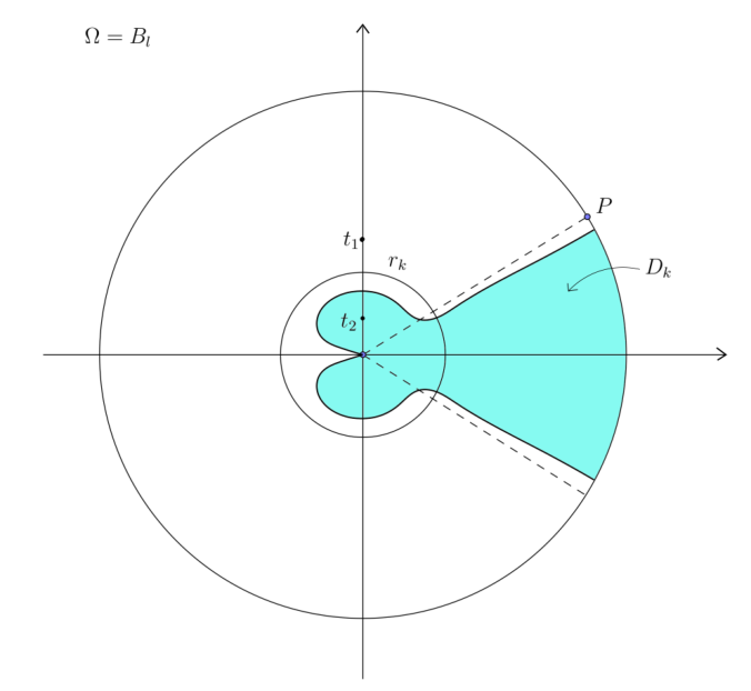
Notice that with strict inclusion whenever is such that . For instance, for we have and , where is a positive small angle; on the other hand4848 48 This is due to the fact that covers the arcs twice, with opposite orientations. . Similarly we have with strict inclusion4949 49 This could only happen for . whenever (thus, ).
The support of the current in (5.6) is a connected set contained in . But in this example we also have ; moreover
The support of the current in (5.17), an orthogonal “wall” over of height , built on , divides into two connected sets; one of them, (see (5.26)), has as part of its boundary, and the other one, (see (5.27)), has as part of its boundary. Hence the support of (Definition 5.13) divides into two connected sets, one of them, , is , and the second one is its complement in and equals . In this particular example the cylindrical Steiner symmetrization introduced in Section 3 is unnecessary, since and hence . Thus the function in (7.1) reads as
Note that
and that is the segment .
Concerning the functions in (6.1), we have , thus , and the sets in (6.4) and in (7.21) are empty. Hence, for in (7.7), we have . Moreover, for in (6.7), we have for ; thus, recalling Definitions 7.7 and 7.12, and since ,
where the last equality follows by construction (see (7.4) and (5.31)).
10.2 An approximating sequence of maps with degree zero: catenoid union a flap
In this section we discuss another example of a possible approximating sequence . We replace the cylinder lateral surface5050 50 In polar coordinates. , which contains the image of through the map in the example of Section 10.1, with half5151 51 For convenience, we consider the doubled segment , in order to define the catenoid; then we restrict the construction to . of a catenoid union a flap (see Fig. 16): calling this union , we have
where and is such that (and ).
Notice that “spans” , which is the union of two unit circles connected by a segment.
Let , be such that as . Set
We define in , in particular
On we define in such a way that for each we have
See Fig. 15 for a representation of the map .

To define on we adopt a construction similar to the one in (10.1). First of all, . Then, in we impose as in (10.1) with replacing . In we require

Hence
Remark 10.2.
For an explicit construction, see Section 13 with and
Now we fix an infinitesimal sequence of positive numbers; we may also assume that . Hence .
By construction there exists such that . Hence for we have
Notice that the above strict inclusions are due to the fact that the segments and are covered twice with opposite orientation.
On the other hand, for we have
where the second inclusion is due to the fact that covers two arcs of twice with opposite orientation. Notice also that the only cancellation that could happen on due to covering more than one with opposite orientation is along the segment , in particular we have
By definition the above equality holds also for ; moreover we have
where .
From the above discussion we can see that the support of the current is a connected set contained in and the support of is a connected set contained in , in particular we have
The current , a normal wall over over of height , built on , divides into two connected sets; one of them, , contains and has as part of its boundary. The other one, (see (5.27)), contains and has as part of its boundary. Hence divides into two connected sets, one of them is
and the second one is its complement in and contains . Note that and that is the segment .
In this particular example when we apply the cylindrical Steiner symmetrization introduced in Section 3 nothing changes, i.e., and hence . Observe that
Thus
and the sets in (6.4) and in (7.21) are empty. Hence
Moreover we have for thus, recalling Definitions 7.7 and 7.12,
The set in Definition 7.14 is empty, hence which is boundaryless in .
10.3 Smoothing by convolution: the case of the two discs
In [1], the authors describe a sequence of maps converging to the vortex map , simply defined as follows:
| (10.2) |
where is a smooth function such that in , in , and . Hence . We shall assume that for all , we have .
Now we fix an infinitesimal sequence of positive numbers, hence for any there exists such that , and we have
| (10.3) |
Notice that ,
Also, using (10.3), and, unlike the examples in Sections 10.1, 10.2, there is no cancellation due to covering the same -dimensional set with two opposite orientations; the fact that is nonempty is due to the fact that is one-dimensional. Moreover we have
Hence
i.e., the current divides into two connected sets; one of them, , and the other one, . Therefore divides into two connected sets, one of them is
and the second one is its complement in and contains .
Also in this example, when we apply the cylindrical Steiner symmetrization introduced in Section 3, nothing changes, i.e., and hence .
Note also that in , thus , and the sets in (6.4) and in (7.21) are empty. Hence . We have for thus, recalling Definitions 7.7 and 7.12,
The set in Definition 7.14 is empty, hence . We have, recalling (8.12),
and
where (see (8.10) (8.4), (8.8), (8.15), and Proposition 8.8)
Notice that
and
Finally we have
where . Notice that
Hence
and
11 Lower bound
In this section we reduce the analysis of in Definition 9.4 to a non-parametric Plateau-type problem with a sort of free boundary. Precisely, after suitable projections, we will arrive to a Plateau-type problem on the closed rectangle , where
in Cartesian coordinates, equivalently in cylindrical coordinates. The rectangle will be often identified with , thus neglecting the third coordinate. We will impose a Dirichlet boundary condition on a part
| (11.1) |
of , while no conditions will be imposed on ; more involved conditions will be assigned on , see the mutual relations between and in (11.23) (see also the problem on the right-hand side of (11.25) and Section 12).
Then the strategy to estimate from below the relaxed area of the graph of the vortex map will be the following: We split
In order to estimate the of the first term on the right-hand side we will employ (4.37), whereas, in order to pass to the limit as in the second term, we will use (9.12), so that we first want to render the right-hand side of this latter inequality independent of . This will be done with the aid of the non-parametric Plateau-type problem studied in this section and in Section 12.
Definition 11.1 (The projection ).
We let be the othogonal projection.
Recall that are defined in (9.8), that is the generalized polar graph of on its domain of definition (see (9.5)), and that takes values in . We first prove the following preliminary result:
Lemma 11.2.
Proof.
The latter assertion follows by symmetry. To prove the former, we argue by slicing. For a.e. the set coincides with support of the current , see [23, Def. 7.6.2]. First notice that for all the conclusion follows by construction5252 52 In this set we have and the current is the integration over the half-circle , whose projection through is the whole interval with endpoints and (in cylindrical coordinates)..
It remains to consider the case . Recall that the set in (9.4) has the form
Therefore, for a.e. the slice is the integration over restricted to the plane , which in turn is the integration over the generalized polar graph (see (2.8)) of restricted to the closed set
Namely
so that the support of can also be obtained as
| (11.3) |
where
For large enough, let
which is a relatively open set in , and let be the slice of on . We have
| (11.4) |
On the other hand since is the boundary of the subgraph of in , it is a closed -integral current in and in , so that the boundary in is supported on . From (11.4), the fact that at and that is constant on the segment with value either or , we deduce that
| (11.5) |
Moreover, if we set
from (11) it follows that
By decomposition of the integral -current (see [15, Section 4.2.25]), there are at most countable Lipschitz curves such that connects to , and is closed for . We claim that there cannot be closed curves , namely . Indeed, since connects and , we see that consists of at least one point for -a.e. . On the other hand, consists of only one point5353 53 Because is the support of a polar graph; the points where this intersection is not a singleton coincide with the values of where has a jump. for -a.e. . So there cannot be other curves otherwise the last condition will be violated.
From the claim we deduce that the current is the integration over a simple curve connecting and , and its support coincides with . Now, from (11.3) and the fact that is a segment on , we conclude that also must be a unique curve, say , connecting to . By continuity of the projection by , is an interval with one endpoint in , for a.e. . ∎
The new coordinates . In what follows, it is convenient to revert the rectangle with respect to its second coordinate: if are the cylindrical coordinates in the cylinder exploited so far, we introduce Cartesian coordinates defined as
| (11.6) |
in such a way that the segment coincides with the bottom edge of the rectangle .
Thanks to Lemma 11.2 we are allowed to give the following
For all for which Lemma 11.2 is valid, we have that equals the length of the interval in (11.2). Now the content of Lemma 11.2 is that the -projection of on is of the form
| (11.7) |
up to a set of zero -measure. The function is built in such a way that and are the endopoints of the interval for almost every . Observe that
and
Indeed, from Definition 9.2, equation (9.4) and Definition 9.4, we see that the set is contained in .
We have built in (9.3) as the set enclosed between and , see formula (9.9). We now perform a (classical) Steiner symmetrization5454 54 Despite is obtained by cylindrical symmetrization, it still can have “holes” (see Fig. 10 for a slice), that disappear when further performing the Steiner symmetrization. of the set with respect to the plane . We denote by the symmetrized set.
Remark 11.4.
We emphasize that the set in is exactly , and is already symmetric with respect to the plane containing . For this reason does not change (in that region) after Steiner symmetrization,
| (11.8) |
Since the perimeter does not increase when symmetrizing, from (9.9) we conclude
| (11.9) |
Definition 11.5 (The function ).
We introduce the function as
| (11.10) |
We stress that the set where is contained, up to -negligible sets, in the region defined in (11.7). Notice also that may take the value in on a set of positive -measure.
Remark 11.6.
- (i)
By definition of classical Steiner symmetrization,
up to Lebesgue-negligible sets, the second equality following from the fact that almost everywhere in ;
- (ii)
since has finite perimeter, it follows that ;
- (iii)
since and is contained in (as a consequence of (9.5)), it follows that has null trace on the segments and .
We can split as
| (11.11) |
up to a set of -measure zero, in such a way that
| (11.12) |
where and are, respectively, the (standard) generalized subgraph and epigraph of in . Notice that, since ,
| (11.13) | ||||
up to -negligible sets.
We are ready to prove the following:
Lemma 11.7.
We have
| (11.14) | ||||
Moreover, .
Proof.
The last assertion follows by symmetry. Let us prove the former: By (11.13) we have
Taking the sum of these two expressions and using (11.9), (11.11), we obtain
Recalling (9.4), we now claim that, up to -negligible sets,
| (11.15) |
see Fig. 10. From the claim it follows that
and hence by (9.10) we conclude
that is (11.14). It remains to show (11.15). As usual, we argue by slicing; hence for almost all we will show that (11.15) holds (up to -negligible sets). Notice that both the left and right-hand sides of (11.15) are empty for , so we assume . Therefore, fix (with ) such that and assume, by contradiction, that . In a first step we will suppose . We might further assume that is a Lebesgue point for the function . Hence in any left-neighbourhood of this point is strictly positive on a set of positive meausure, i.e., we can find positive numbers such that for all , there exists a set , of positive measure such that
| (11.16) |
If is the projection in Definition (7.5), since for small enough the segment satisfies
We have that is a homeomorphism. Now, if the segment cannot intersect the subgraph of (on a set of positive -measure), and thus
| (11.17) |
where represents the usual angular coordinate. Since is infinitesimal as , condition (11.17) contradicts (11.16).
Let us now treat the case . This is much simpler to deal with, up to noticing that is defined on . The fact that means that the line does not intersect on a set of positive -measure but this contradicts the fact that . Indeed since hence there exists such that . Let then a suitable rotation of around the axis of the cylinder shall meet on a set of positive -measure (note that ), which contradicts ∎
Remark 11.8.
Remark 11.9.
Recalling the expression (11.1) of , define as
| (11.21) |
Definition 11.10 (The functional ).
Given and we define
| (11.22) |
We further define
| (11.23) |
Remark 11.11.
- (i)
The Borel function satisfies in , and is such that almost everywhere in . Moreover , and . In particular
- (ii)
if , and if is smaller than almost everywhere on then the last addendum on the right-hand side of (11.22) vanishes.
- (iii)
Notice that in minimizing we have a free boundary condition on the edge . By Remark 11.11 (i) and (11.24) we have
| (11.25) |
which leads to the investigation of the minimum problem on the right-hand side.
Remark 11.12.
Let . If is a Lebesgue point for , and if , then the trace of over the segment vanishes. Indeed for any we can find such that
| (11.26) |
Let now be such that (i.e., ), and set . By Chebyschev inequality and (11.26) it follows that the set satisfies
| (11.27) |
Then, for any we infer5555 55 In the first inequality we have used that ; in the second inequality that is the subgraph of in ; in the third inequality we have used that and that .
| (11.28) | ||||
where the penultimate inequality follows from the inclusions
and the last inequality follows from (11.27). Now (11.28) entails the claim by the arbitrariness of and since .
We now refine the choice of the class of pairs where the infimum in (11.25) is computed.
Definition 11.13 (The classes and ).
We set
Proposition 11.14 (Convexifying ).
We have
| (11.29) |
Proof.
It is enough to show the inequality “”. By extending outside as in , we see that
| (11.30) |
where, with a little abuse of notation,
being the trace of on .
The thesis of the proposition will follow from the next three observations:
- (1)
If is such that for some Lebesgue point , then the subgraph of splits in two mutually disjoint components: and . Let be such that
The trace of over the segment is , as a consequence of Remark 11.12. Then the function defined as
still satisfies , and
Being identically zero in , in particular in , we can introduce
so that and we easily see that ; hence
- (2)
More generally, let and let be any Lebesgue point of ; we can also suppose that . Consider
(11.31) We claim that Define
that is the set where we have replaced by . To prove the claim, using (11.30) and the equalities
we have to show that
(11.32) Assume that is non-empty and that . It is convenient to introduce
so that is an open rectangle. Since we have modified only in , inequality (11.32) is equivalent to
(11.33) with (resp. ) the external and internal traces of (resp. ) on ; here we have used from Remark 11.12 that the trace of on is zero (hence ) and that the external traces , on vanish as well. Hence, exploiting that on , so that , and that on , inequality (11.33) is equivalent to
(11.34) We split
with , , and . Since , by slicing and looking at as an integral current, we have5656 56 Here we use that in .
where is the slice of on the plane , that is the generalized graph of the function . From the above expression, the triangular inequality implies (11.34).
- (3)
Let . Let be Lebesgue points for with , and let . We consider the following modifications of and :
and
In other words we set equal to above the segment connecting to . Also in this case we have
(11.35) Indeed, if the proof is identical to the case (2). Otherwise, it can be obtained by slicing as well, parametrizing by an arc length parameter, then slicing the region 5757 57 represents the affine function whose graph is . by lines perpendicular to , and exploiting the fact that equals zero on the segments .
Let be given; from (3) we can always replace by its convex envelope and modifying accordingly , we get two functions and such that (11.35) holds. Moreover, by (2), if is a Lebesgue point for , we can always replace by in (11.31), so that turns out to be nonincreasing. The assertion of the proposition follows. ∎
Let us rewrite the functional in a convenient way. Let , and let be the graph of . We have, using (11.22),
| (11.36) |
where, in the integral over , we consider the trace of on .
Corollary 11.15.
Let and . Then for any we have
| (11.37) |
for an absolute constant , and where the sequence depends on and and is infinitesimal as .
Proof.
11.1 Lower bound: reduction to a Plateau-type problem on the rectangle
We now state and prove our first main result.
Theorem 11.16 (Lower bound for the area of the vortex map).
The relaxed area of the graph of the vortex map satisfies
| (11.39) |
Proof.
We write
Therefore
| (11.40) |
Given and , from (4.37) it follows
| (11.41) |
From (11.37) we have
| (11.42) |
Exploiting the fact that the right-hand side of (11.38) does not depend on , we can pass to the liminf as in the above expression, to obtain
| (11.43) |
From (11.40), (11.41) and (11.43) we obtain
| (11.44) |
for all and . Letting and then , by the dominated convergence theorem (since as ) we get
∎
12 Structure of minimizers of
In this section we analyse the minimum problem on the right-hand side of (11.29). We prove the existence of minimizers, and exploy it to show that the inequality (11.39) in Theorem 11.16 is optimal. First it is convenient to write the analogue of in a doubled rectangle, see (12.4).
We start by introducing some notation. We denote the open doubled rectangle, , and define its Dirichlet boundary5858 58 Note that consists of three edges of , while (see (11.1)) consists of two edges of . as
so that .
Definition 12.1.
We set
| (12.1) |
For each , we further define
where in the case . We set
| (12.2) |
which is either empty, or the union of two equal intervals, see Fig. 17.

Define
| (12.3) |
The graph of on consists of two half-circles of radius centered at and respectively, see Fig. 18. We notice that such a extends definition (11.21).

Definition 12.2 (The functional ).
We define
and for any ,
| (12.4) |
Remark 12.3.
- (i)
The only case in which the last addendum on the right-hand side of (12.4) may be positive is when is identically on ;
- (ii)
We have
(12.5) where
(12.6) and denotes the trace of from the side of . To show (12.5), we start to observe that, using that on , it follows . This last term is nonzero only if , in which case is empty, and the equivalence between (12.4) and (12.5) easily follows. If instead is not identically , then, using again that on , we see that the last term on the right-hand side of (12.4) is null, and
(12.7) Hence, if is not identically , inserting (12.7) into (12.4), we obtain, splitting , and using that on ,
- (iii)
We have
(12.8) - (iv)
If everywhere, then is connected, , and the sum of the first three terms on the right-hand side of (12.5) gives the area of the graph of on , with the boundary condition set to be on .
- (v)
Our aim is to have a surface in , of graph type, whose boundary consists of the union of the graph of and the graph of a convex function . The last three terms in (12.5) are an area penalization to force the solution to attain these boundary conditions by filling, with vertical walls, the gap between the boundary of any competitor surface (the generalized graph of ) and the required boundary conditions. In particular the presence of the last term of (12.5) is explained as follows: assume that , i.e., ; the graph of any does not reach the graph of (simply because ). To overcome this, the graph of is glued to the wall consisting of the subgraph of (inside ).
- (vi)
Take , and on , then , , and , , hence
that is the functional in some sense forces a minimizing sequence to attain the boundary conditions as much as possible.
By symmetry, we easily infer
| (12.9) |
therefore we can now restate the content of Theorem 11.16 as follows:
| (12.10) |
Remark 12.4 (Two explicit estimates from above).
In the next section we shall prove the existence and regularity of minimizers for the minimum problem on the right-hand side of (12.10).
12.1 Existence of a minimizer of
The construction of a suitable recovery sequence for the relaxed area of the graph of the vortex map depends on the existence and regularity of one-codimensional area minimizing surfaces of graph type for problem (12.9). We start by analysing the features of the space in (12.1). Clearly the graph of is symmetric with respect to ; also, the convexity of implies , and has a continuous extension on .
Lemma 12.5 (Compactness of ).
Every sequence has a subsequence converging uniformly on compact subsets of to some element of .
Proof.
See for instance [22, Sec. 1.1]. ∎
It is convenient to extend in the doubled rectangle by defining the extension as:
| (12.13) |
In the rest of this section we want to prove the following result.
Theorem 12.6 (Minimizing pairs).
There exists such that
| (12.14) |
and is symmetric with respect to . Moreover, if is not identically , then
- (i)
, and in ;
- (ii)
is locally Lipschitz (hence analytic) and strictly positive in ;
- (iii)
is continuous up to the boundary of , and attains the boundary conditions, i.e., for ,
(12.15) hence
(12.16) - (iv)
we have
(12.17)
The rest of this section is devoted to prove this theorem; we start with some preparation.
Definition 12.7 (Convergence in ).
We say that a sequence converges to , if
- -
converges to uniformly on compact subsets of ;
- -
converges to in .
Lemma 12.8 (Closedness of ).
Let be a sequence such that converges to uniformly on compact subsets of , and converges to in . Then .
Proof.
Possibly passing to a (not relabelled) subsequence, we can assume that converges to pointwise in , with , and in for all . We only have to show that in . We can also assume that does not intersect the graph of . If , then . From the local uniform convergence of to in it follows that for large enough, i.e., , and the assertion follows. ∎
Lemma 12.9 (Lower semicontinuity of ).
Let be a sequence converging to in the sense of Definition 12.7. Then
| (12.18) |
Proof.
It is standard5959 59 Indeed, let be defined as on , and on . Let be an open disc containing . We extend to a function in , [19, Thm. 2.16], and we still denote by such an extension. For every , define in and in . We have where the last equality follows from [19, (2.15)]. Thus the lower semicontinuity of the functional in (12.19) follows from the -lower semicontinuity of the area functional. to show that the functional
| (12.19) |
is -lower semicontinuous. Since converges to pointwise in , we also have . The assertion follows. ∎
Proof.
We now turn to the regularity of minimizers.
Proposition 12.11 (Analyticity and positivity of a minimizer).
Suppose that is a minimizer of (12.14), and that is not identically . Then is analytic in , and solves the equation
| (12.21) |
Moreover in .
Proof.
Since by assumption is not identically , we have that is nonempty. Moreover minimality ensures
for any , . Thus, by [19, Thm 14.13], is locally Lipschitz, and hence analytic, in , and (12.21) follows. Now, let and take a disc . Since on we find, by the strong maximum principle [19, Thm. C.4], that either is identically zero in , or in . Hence from the analyticity of and the arbitrariness of , we have that either is identically zero in or in . Now , see (12.11). Thus is not a minimizer, and the positivity of in is achieved.
∎
Lemma 12.12 (Symmetric minimizers).
There exists a minimizer of (12.14) such that and is symmetric with respect to .
Proof.
Let be a minimizer of (12.14). Let be an open interval; consistently with (12.4), and since is continuous in , we set
Recall that , hence its graph is symmetric with respect to . Define on and for , in particular the graph of is symmetric with respect to . Since , it follows for, if , then which contradicts the minimality of . ∎
Lemma 12.13.
Suppose that is a minimizer of (12.14) such that:
- (i)
;
- (ii)
is symmetric with respect to ;
- (iii)
is not identically .
Then
Proof.
By the symmetry of and with respect to (Lemma 12.12) we may restrict our argument to . Assume by contradiction that there exists such that . Recall that is convex, nonincreasing in and continuous at . Let
Since is not identically , we have , and is strictly decreasing in . Let
be the inverse of . We have, using (12.5) and (12.6),
Now, we argue by slicing the rectangle with lines . Recalling the expression of (which is non empty by assumption (iii)), and neglecting the third addendum,
where stands for the partial derivative with respect to . Neglecting in the third addendum on the right-hand side, we deduce
Hence the value of on the pair , is smaller than , thus contradicting the minimality of . ∎
We now prove point (iii) of Theorem 12.6: this will be a consequence of the next lemma and Theorem 12.16.
Lemma 12.14.
Let be as in Lemma 12.13. Then attains the boundary condition on .
Proof.
The result follows from [19, Theorem 15.9], since is union of three segments. ∎
Remark 12.15.
The conclusion of the proof of Theorem 12.6 (iii) is given by the following delicate result.
Theorem 12.16.
Proof.
By Remark 12.15, we can assume that is not identically and, by Lemma 12.13, also that for any . Therefore, fix a number and set
We extend in as follows: we define , in , and
In this way is continuous in .
Now, we divide the proof into six steps. We start by regularizing (step 1) in order that the regularized functions have smooth graphs (hence of disc-type6060 60 We expect the graph of , considering also a possible vertical part over the graph of , to be a surface of disc-type; however, we miss the proof of this fact, mainly due to possible high degree of irregularity of the trace of over .). Next (step 2), we will compare these graphs with the solution of a suitable disc-type Plateau problem.
Step 1: Approximation of . Let be a natural number (that will be sent to later) such that , and consider the enlarged rectangle
| (12.22) |
see Fig. 19. Note that
Given , we claim that we can build a sequence (depending on ) which satisfies the following properties:
| (12.23) | ||||
In order to obtain these features for we use standard arguments (details can be found in [2, Thm. 3.9] or [18, Thm. 1, Section 4.1.1]). To the aim of our discussion, we just recall that we proceed by constructing an increasing sequence of subsets of , , , (for we take for definitiveness) and with the aid of a partition of unity associated to , for , we mollify accordingly in . For our purpose we choose6161 61 We need the full set as support in order that the argument to detect the behaviour of (defined in (12.32)) in applies. in such a way that
| (12.24) |
Since is obtained by mollification we have and moreover because it attains the continuous boundary datum on . Notice that we use the same mollifier in each , choosing with , decreasing with respect to , with6262 62 and depend on . We could take . as . Finally, , and for . It follows
| (12.25) |
Using [18, Prop. 3 Sec. 4.2.4 pag. 408, and Th. 1 Sec. 4.1.5 pag. 331] we infer
| (12.26) |
Now that properties (12.23) are achieved, by a diagonal argument we select functions such that
| (12.27) | ||||
On the basis of (12.26) and (12.27), we can also ensure6363 63 To prove claim (12.28), fix , and set outside and in , so that Then , the first equality following from the strict convergence of to [18, Prop. 3 Sec. 4.2.4 pag. 408 and Thm. 1 Sec. 4.1.5 pag. 371]. Taking the limit as , since we conclude . Then (12.28) follows by lower-semicontinuity. that
| (12.28) |
Here, by we mean the area of the graph of relative to the closed rectangle , which, recalling also Proposition 12.11, reads as
| (12.29) |
where denotes the trace of on .
We now construct functions such that
| (12.30) | ||||
where
| (12.31) |
and finally
For any we define
| (12.32) | ||||
Since (see Proposition 12.11) is positive in it turns out, recalling also that is obtained by mollification, that
| (12.33) | ||||
Also, in , and in . Moreover, again the positivity of implies that
| (12.34) |
whereas
| (12.35) |
because if , and if . Exploiting (12.25), and the fact that is nonincreasing (resp. nondecreasing) in (resp. in ), one checks6464 64 Let us show for instance that is decreasing in . Recall that the function vanishes above the graph of , which is decreasing in . Now, take a point , , ; suppose first that . If , then , and if , then . Hence, if then also for small enough, because , being decreasing in . This argument applies also when , by (12.25), since is nonincreasing also in . that also is nonincreasing in (and nondecreasing in ). Concerning the behaviour of in (and similarly in ), we see that in (), we are mollifying with whose radius of mollification is , so that equals on the line , and nonzero below inside (this follows from the fact that is on the line and nonzero below). We have defined the radii in such a way that they are decreasing with respect to , so that, being the sum of (whose support is by (12.24)), it turns out that is on and nonzero below6565 65 Notice that in only and , are nonzero. in (from this it follows that in ). In particular is piecewise constant and nondecreasing in .
Therefore we have
| (12.36) |
Finally, it is not difficult to see that the functions converge to in as , and
| (12.37) |
From this, (12.28), Lemma 12.14, (12.29) and (12.4) we deduce
| (12.38) |
Step 2: Comparison with a Plateau problem. In this step we want to compare the graph of with the solution of a disc-type Plateau problem. In particular we will obtain a disc-type surface whose area is smaller than or equal to the area of the graph of , see (12.39). In step 3 (see (12.41)) we will compare this surface with the graph of on .
We recall that is continuous in , it is positive on the bottom edge of (see (12.27)), it is zero on the top edge by (12.33), and on the lateral edges of it coincides with ; more specifically
Define
From (12.27), we see that coincides with over , and its graph over this set is a curve, that we denote by . This curve, excluding its endpoints and , is contained in the half-space , while . We further denote by the symmetric of with respect to the plane , so that
is a Jordan curve in , see Fig. 19. We can now solve the disc-type Plateau problem with boundary [14] and call one of its solutions6666 66 is the image of an area-minimizing map from the unit disc into .. Finally, we can assume that is symmetric with respect to and that
with , respectively (see Fig. 19).

We now want to compare the area of the graph of in with . To this aim we start by observing that , being smooth in and continuous in , is such that its graph over has the topology of , that is the topology of the disc6767 67 is bounded by construction, and it is open from (12.34), (12.35). In addition, it is connected and simply connected. Indeed, take any continuous curve . Using (12.33), let be such that ; hence we can (vertically) contract continuously to its projection on the line , and then contract it continuously to the middle point of , showing that is homotopic to the constant curve. Hence, by the Riemann mapping theorem, is biholomorphic to the open unit disc, and is homeomorphic to the closure of the disc, thanks to the fact that is a Jordan curve, due to the BV-regularity of . . Denoting by the graph of over , we consider the graph of over , and observe that the closure of is a disc-type surface with boundary . Therefore, by minimality,
| (12.39) |
Step 3: Passing to the limit as : the surface . The graph of over the segment and the graph of over the two segments form a simple continuous curve which, excluding the two endpoints and , is contained in the half-space , while (see Fig. 19). If we consider
with the symmetric of with respect to , a direct check shows that the curves converge to the curve in the sense of Frechet [27], as . As a consequence, the area-minimizing disc-type surfaces satisfy (see [27, Paragraphs 301, 305]), with a disc-type area-minimizing surface spanned by . It follows
| (12.40) |
where . From (12.40), (12.39), (12.38) we deduce
Since on , we get
| (12.41) |
Let be a parametrization of , which is analytic and conformal in the open unit disc and continuous up to with . Exploiting the results in [25] (see also [14, pag. 343]) we know that
| (12.42) |
since is a simple curve on the boundary of the convex set .
Now, we need to prove several qualitative properties of .
Step 4: is a simple curve connecting and . This can be seen as follows: Assume and for two distinct points . By standard arguments6868 68 See also step 5 where a similar statement is proved., the disc is splitted into two connected components and and the set must be a simple curve in connecting and (here we use that the points and are the unique points in where and that the two arcs in with extreme points and are mapped in and respectively). By the injectivity of (property (12.42)) we conclude that
| (12.43) |
is a simple curve connecting and on the plane , and more specifically .
In the next step we show that, due to the particular form of , the surface admits a semicartesian parametrization [8], namely that if we slice with a plane orthogonal to the first coordinate (in ) then the intersection is a curve connecting the two corresponding points on ; in addition, in this present case, this curve turns out to be simple. We will also show that the free part of , i.e., , leaves a trace on which is the graph of a convex function (of one variable).
Step 5: The projection of on the plane is the subgraph of a convex function .
We first show that is the subgraph of a function , and then we prove that . Take a point ; by the strong maximum principle, (this follows since points in are in the interior of the convex envelope of , see [14]). Consider the (unique) point such that . Due to the particular structure of , one easily checks that splits into two connected components, and , since consists of two points , in . In particular, the continuous function changes sign only twice on , namely at and . From Rado’s lemma [14, Lemma 2, pag. 295] it follows that there are no points on where the two area-minimizing surfaces and the plane are tangent to each other6969 69 If is a tangence point, then the differential of must vanish at .. It follows that, if , then the set is, in a neighbourhood of , an analytic curve, see again [14, Lemma 2, pag. 295]. Hence, is, in a neighbourhood of , an analytic curve. If is a parametrization of this curve, a bounded open interval, we see that the limits as and of exist7070 70 is compact, hence has some accumulation point as . Notice that and are homeomorphic by contruction; in turn is homeomorphic to the analytic curve . Assume is an accumulation point for as . If , there is a small neighborhood of such that is an analytic curve. Then , in a right neighbourhood of , is homeomorphic to the analytic curve emanating from , which in turn is the restriction of . In particular is a curve emanating from and the limit as of is . If instead then must be the unique accumulation point. Indeed, , and then or (say ). Assume there is another accumulation point as ; then , otherwise we fall in the previous case, and therefore necessarily . But in this case, we see that there must be another accumulation point (as , we move between a neighbourhood of and a neighbourhood of frequently, so that there should be some other accumulation point in ) leading us to the previous case again. and are points in . If belongs to , it must be either or , if instead it is in , then we can always extend in a neighbourhood of and find a larger interval on which can be extended. Similarly, for . Let now be a maximal interval on which is defined, so that, by maximality, the limits as and are and , respectively. We can then consider the closure of and we have that is a curve in joining and . Thus we have proved that equals . In particular is a curve in contained in the plane and connecting the points and . But we know that , so is a segment in with endpoints and for some , and . In particular the whole segment “below” , namely the one with endpoints and , belongs to , and is then the subgraph of some function . As a remark, due to the symmetry of the curve , we can assume is symmetric with respect to , namely .
Now we show that is convex. Assume it is not, and take two points , such that there is a third point , with , which is strictly above the segment in joining and . Let be a nonzero affine function7171 71 Take the signed distance from the plane. vanishing on the plane passing through and orthogonal to , and assume that is positive at . Let be such that . Then is harmonic, and by the maximum principle there is a continuous curve in joining to such that is always positive on . But now, the continuous curve joins to and remains, in , strictly above the segment . This is a contradiction, because must be in the interior of the subgraph of .
Before passing to step 6, recall the definition of in (12.43), and observe that the Jordan curve is the boundary of the disc-type surface . Let us denote by the connected component of with boundary .
We are now in a position to show that admits a non-parametric description over the plane .
Step 6: Graphicality of : the disc-type surface can be written as a graph over the plane of a function . At first we observe that if is not Cartesian with respect to , then there is some point where the tangent plane to is vertical7272 72 This can be seen as follows: as shown in step 5, the intersection between and any plane , , is a simple curve with endpoints in . If is not Cartesian, one of these curves is not Cartesian, and then there is a point where the tangent vector to is vertical. At such a point the tangent plane to is vertical. , that is, it contains the line . We will show, with an argument similar to the one needed to prove Rado’s Lemma [14, Lemma 2, pag. 295], that any vertical plane is tangent to in at most one point.
- Claim:
If is a vertical plane which is tangent to , then there is at most one point where and are tangent.
Assume intersects the relative interior of . It is easy to see that the intersection between and the Jordan curve consists at most of four points7373 73 A vertical plane intersects on a straight segment. In turn, this segment intersects in two points. If a vertical plane intersects in a point , then . Moreover this plane intersects also at . Thus, the points of intersection are at most four. The degenerate cases in which contains a full -measured part of are excluded by this analysis, because in these cases does not intersect the interior of . Instead, the cases in which the intersection consists of or points are easier to treat, and we detail only the -points case (notice that by the geometry of , the case of points occurs when this plane is tangent to at one of the points or ). , . Let be a linear function on vanishing on . Then is harmonic in and continuous in ; in addition, it vanishes at , and alternates its sign on the four arcs on with endpoints . With no loss of generality, we may assume on and . By harmonicity of , any connected component of the region must contain part of or , so that we deduce that these connected components are at most two.
Assume now by contradiction that there are two distinct points and of such that is tangent to at and . Since has null differential at and , the set , in a neighbourhood of , consists of analytic curves crossing at , whereas in a neighbourhood of , it consists of analytic curves crossing at . Therefore, in a neighbourhood of , the set counts at least open regions (and similarly at ). Let us call the two of these regions , and , (’s around and ’s around ). By harmonicity each and must be connected to one of the arcs or . Hence some of these regions must belong to the same connected component of . Then we are reduced to two following cases (see Fig. (20)):
- (Case A)
and belong to the same connected component (say the one containing ). Hence we can construct two disjoint curves in , both joining to a point in , emanating from , one in region and one in region . This contradicts the maximum principle, because these two curves would enclose a region where takes also negative values, whereas its boundary is in .
- (Case B)
and are joined to and and are joined to . In this case we can construct four curves in : and emanating from in regions and and reaching and , respectively; and emanating from in regions and and reaching and , respectively. The region enclosed between these curves has boundary contained in and necessarily inside it the function takes also negative values, again in contrast with the maximum principle.
From the above discussion our claim follows.
We are now ready to conclude the proof of step 6: suppose by contradiction that is not Cartesian with respect to , and take a point where the tangent plane to at is vertical. By symmetry of , the point , defined as the symmetric of with respect to the rectangle , belongs to , and the tangent plane to at is the same plane . This contradicts the claim. We eventually observe that is analytic on the subgraph of , since its graph is . We conclude that belongs to , since also its total variation is bounded by the area of its graph, which is finite.

Step 7: the pair is an admissible competitor for . To see this, we recall that in step 5 we proved that is convex and , i.e. . Furthermore is the graph of , and its projection on the plane is the subgraph of . It follows that the area of the graph of is exactly the area of upon . Let us also recall the regularity of proved in step 6. Setting in we infer the admissibility of .
Step 8: Conclusion. From (12.41) we deduce
| (12.44) |
where the last equality follows from the fact that is continuous on . Hence, also is a minimizer for . We now show that is continuous and equals on . Indeed is analytic, hence also is smooth (and convex). Moreover we know that is smooth in . If its trace on is strictly positive somewhere, we infer that the vertical subset of defined as
has positive -measure and cannot have zero mean curvature (the only case in which its mean curvature vanishes is when is linear, but in this case must be contained in a plane containing which is impossible, since is not). We conclude on . Finally, for, if not, the vertical part of obtained on is flat and then, by analyticity, also is, a contradiction. The thesis of the theorem, and hence of Theorem 12.6 (iii), is achieved. ∎
To conclude the proof of Theorem 12.6, it remains to show (iv). The pair , where the function is as in (12.13), is one of the competitors for problem (12.14) (notice that attains the boundary condition); in addition, its subgraph is strictly convex (see Fig. 18), hence7474 74 As observed, the minimal surface is the graph of , and it must be contained in the convex envelope of , i.e., inside the subgraph of . necessarily in (where we have taken , the solution given by Theorem 12.16).
Eventually, the strict inequality in (12.17) is a consequence of the strong maximum principle: indeed, the internal points of a minimal surface are always strictly inside the convex hull of its boundary, with the only exception in the case of part of a plane (see [27, pag 63, section 70]); so that internal points of are strictly inside the the graph of (that is half of the lateral boundary of a cylinder). ∎
We conclude this section by observing a consequence of Theorem 12.16: Let be the graph in of a function such that , and consider the curve obtained by concatenation of with the graph of over .
Corollary 12.17.
We have
| (12.45) |
where is a minimizer of , is a parametrization of a disc-type area-mininizing solution of the Plateau problem spanning (see (2.9)), and the infimum is computed over all functions as above.
13 Upper bound
A minimizer of (12.14) needs to be used for constructing a recovery sequence , see formulas (13.25) and (13.27): we know that is locally Lipschitz, but not Lipschitz, in ; therefore we need first a regularization procedure.
Let be a minimizer provided by Theorem 12.6, and assume that is not identically . We fix an integer and, recalling the definition of in (12.13), define
| (13.1) |
We observe that is Lipschitz continuous in . We then set
| (13.2) |
Since is locally Lipschitz in , an easy check shows that is Lipschitz continuous in for any (with an unbounded Lipschitz constant as ). This follows from the fact that is continuous up to the boundary of (see Theorem 12.6 (iii)) and hence coincides with either or in a neighbourhood of in . Furthermore still on the upper graph of .
Lemma 13.1 (Properties of ).
Proof.
(i) and (ii) are direct consequences of the definitions. To show (iii) we start to observe that pointwise in : indeed, this follows from the definitions of and up to noticing that pointwise in as , and on . From Theorem 12.6 (iv) it follows that, at any point , for large enough (since ), so that . As a consequence the set satisfies
and on it holds and . Moreover, on , either (and hence ) or (and hence ). Therefore
and
because are uniformly bounded in . Also
and (13.3) follows. ∎
The main result of this section reads as follows.
Theorem 13.2 (Upper bound for the area of the vortex map).
The relaxed area of the graph of the vortex map satisfies
| (13.4) |
Proof of theorem 13.2.
To prove the theorem, we need to construct a sequence converging to in such that
where is a pair minimizing as in Theorem 12.6. We can assume that is not identically , otherwise the result follows from [1].
We will specify various subsets of and define the sequence on each of these sets (see Fig. 21). More precisely, we will define as a map into in the largest sector (step 1). This construction is similar to the one in [1] (see also Remark 13.3 below). The contribution of the area in this sector will equal, as , the first term in (13.4). The second term will be instead provided by the contribution of in region (step 2), where we will need the aid of the functions (suitably regularized, in order to render Lipschitz continuous). The other regions surrounding are needed to glue between the aforementioned regions. This is done in steps 3, 4 and 5, where it is also proven that the corresponding area contribution is negligible. Finally, in steps 6 and 7 we show the crucial estimates to prove (13.4). In Fig. 21 this subdivion of the domain is drawn.
Remark 13.3.
Our construction differs from the one in [1], even when in place of we use (i.e., the one in Section 10.1) in the following sense. We use the full graph of to construct (and therefore, in the case when is replaced by , the image of covers the whole cylinder and not only a part of it). Since may be not identically (and actually is not explicit in general), the presence of a new set is now needed, as an intermediate region to glue the trace of along two segments . The image set covers a small part of the unit circle. See Fig. 21.
Let and let be infinitesimal sequences of positive numbers such that . We shall suppose7575 75 This assumption will be used only in step 7.
| (13.5) |
Let be the open disc centered at the origin with radius , and
| (13.6) |
be the half-cone in , with vertex at the origin and aperture equal to , see Fig. 21. Let
| (13.7) |
We set
and divide into two sets
| (13.8) |

Step 1. Definition of in .
In this step our construction is similar to the one in [1, Lem. 5.3], see also (10.1); in order to define , in the source we use polar coordinates and in the target Cartesian coordinates. Define
| (13.9) |
Observe that
| (13.10) |
The relevant contribution to the area of the graph of is the one in region , and more specifically in ; it is in this region that we need to use a minimizing pair of .
Step 2. Definition of on .
We first need a regularization of : assuming without loss of generality , we define
| (13.11) |
where we recall that (see Theorem 12.6), and we set for (see Fig. 21, right). Notice that , and the convexity of implies that also is convex, , and therefore by Lemma 13.1 (i) we see that , where is the approximation of in Lemma 13.1 (with ), see formula (13.2). Again by Lemma 13.1, as .
We start with the construction of on . Set
| (13.12) | ||||||
| (13.13) |
Note that is a bijective increasing function, for any . Thus
| (13.14) | ||||
| (13.15) | ||||
| (13.16) |
We have, for all and ,
| (13.17) | ||||
| (13.18) |
and, for almost every and all ,
| (13.19) |
Moreover we define
| (13.20) |
to be the inverse of and, recalling that ,
| (13.21) |
Notice that is a linearly decreasing bijective function.
The map
| (13.22) |
is invertible, and its inverse is the map
| (13.23) |
The modulus of the determinant of the Jacobian of is given by
| (13.24) |
We set
| (13.25) |
Observe that, using the definition of ,
| (13.26) | ||||
for and , as it follows from (13.12), (13.14), (13.15), and (12.15), where is defined in (13.1) (with ).
Eventually we define on as
| (13.27) |
It turns out
for , .
The area of the graph of on will be computed in step 7.
Step 3. Definition of on and its area contribution.
Let (resp. ) denote the graph of (resp. of ) on . We introduce the retraction map , , defined by
where is the line passing through and . Then is well-defined and it is Lipschitz continuous in a neighbourhood of in . We also define
as the restriction of to ; see Fig. 22. As a consequence, since for large enough is contained in a neighbourhood of , we have that is Lipschitz continuous with Lipschitz constant independent of . Notice also that and .
We define on setting, for and ,
We have
so that glues, on , with the values obtained in step 2 (last formula in (13.26)), and
This formula shows that also glues, on , with the values obtained in step 2 (second and third formula in (13.26)). Moreover
| (13.28) |
In addition, the derivatives of satisfy, for and , using (13.16),
so that
where is a positive constant independent of , which bounds the gradient of . Since is Lipschitz, we deduce that is Lipschitz continuous7676 76 The Lipschitz constant of on this set turns out to be unbounded with respect to . on .
Furthermore the image of through the map is the region enclosed by and (with multiplicity ). The area of this region is infinitesimal as , so that, by the area formula,
Hence, using the fact that the gradient in polar coordinates is , we eventually estimate (see also (2.3))
| (13.29) |
as . In the last equality we use that , which is integrable via the change of variables (it also makes disappear at the denominator in front of the integral in (13)).
This proves that the contribution of area of the graph of over is infinitesimal as .

Eventually, for , , we set
| (13.30) |
Observe that, thanks to (13.27), is continuous on , and similar estimates as in (13) for the area hold on .
Step 4. Definition of on and its area contribution.
We start with the construction of on . For and we set
| (13.31) |
First we observe that
so that is continuous on (see (13.28) and (13.16)), and
| (13.32) | ||||
| (13.33) |
Direct computations lead to the following estimates:
| (13.34) | ||||
| (13.35) |
where is the constant bounding the gradient of as in step 3. Finally, since by (13.31) takes values in , we have for all , . Hence, the area of the graph of on is
where is a positive constant independent of . Exploiting that , we can estimate the right-hand side of the previous formula as follows:
| (13.36) | ||||
where as , and is a positive constant independent of which might change from line to line.
In we set, for , ,
Similar estimates as in (13.36) for the area hold on .
Step 5. Definition of on and its area contribution.
We first construct on . We define as
where
Notice that is decreasing and takes values in . Therefore we set
One checks that , (see also (13.9)), and
Notice also that is continuous at and . Finally, since takes values in , the determinant of its Jacobian vanishes, so that in order to estimate the area contribution of the graph of in it is sufficient to estimate the derivatives of . We have
Therefore
| (13.37) |
with as . Notice that the integral of with respect to can be computed via the fundamental integration theorem, since is monotone.
In we set
We now define on . We set
Then , and
Hence
| (13.38) |
as .
Step 6. We claim that
| (13.39) |
where we recall that
Indeed, on the maps and take values in the circle , hence
Thus
From (13.9), we have
| (13.40) | ||||
Our previous remarks and the fact that as , imply (13.39).
Step 7. We know from (13), (13.36), (13), and (13.38), that the integral of is infinitesimal as , on the region . Therefore it remains to compute the area of the graphs of in the region . We claim that this contribution is
| (13.41) |
To prove this, we start to compute the area of the graph of restricted to . From (13.25), (13.17), (13.19) and (13.18), we have
| (13.42) | ||||
where denotes the derivative of with respect to , are evaluated at , and the two partial derivatives , of with respect to are evaluated at . Note carefully that, in the computation of the Jacobian, the terms containing cancel each other.
Notice that, since is convex, its derivative is nonincreasing, and therefore . As a consequence of (13.42), from (2.3), we have
where , are evaluated at , and , are evaluated at . Now we use the change of variable (13.22): from (13.24), we have
where , are defined in (13.20), (13.21), is evaluated at , and and are evaluated at . Therefore
| (13.43) |
where
Since and , we deduce from (13.20), (13.21),
Therefore we see that
as . Moreover
| (13.44) |
as . Indeed we may estimate
and using that (see (13.11)), if we assume (13.5), i.e., , then (13.44) follows, since the -norm of is bounded uniformly with respect to .
Corollary 13.4 (Minimizers for large enough).
For large enough, a solution to the minimum problem on the right-hand side of (12.9) is given by and .
Acknowledgements
The first and third authors acknowledge the support of the INDAM/GNAMPA. The first two authors are grateful to ICTP (Trieste), where part of this paper was written.
References
- [1] E. Acerbi and G. Dal Maso, New lower semicontinuity results for polyconvex integrals, Calc. Var. Partial Differential Equations 2 (1994), 329–371.
- [2] L. Ambrosio, N. Fusco and D. Pallara, “Functions of Bounded Variation and Free Discontinuity Problems”, Mathematical Monographs, Oxford Univ. Press, 2000.
- [3] J.M. Ball, Convexity conditions and existence theorems in nonlinear elasticity, Arch. Ration. Mech. Anal. 63 (1977), 337-403.
- [4] J.M. Ball and F. Murat, -Quasi-convexity and variational problems for multiple integrals, J. Funct. Anal. 58 (1984), 225-253.
- [5] G. Bellettini, A. Elshorbagy, M. Paolini and R. Scala, On the relaxed area of the graph of discontinuous maps from the plane to the plane taking three values with no symmetry assumptions, Ann. Mat. Pura Appl. 199 (2019), 445–477.
- [6] G. Bellettini and M. Paolini, On the area of the graph of a singluar map from the plane to the plane taking three values, Adv. Calc. Var. 3 (2010), 371–386.
- [7] G. Bellettini, M. Paolini and L. Tealdi, On the area of the graph of a piecewise smooth map from the plane to the plane with a curve discontinuity, ESAIM: Control, Optimization and Calculus of Variations 22 (2015), 29–63.
- [8] G. Bellettini, M. Paolini and L. Tealdi, Semicartesian surfaces and the relaxed area of maps from the plane to the plane with a line discontinuity, Ann. Mat. Pura Appl. 195 (2016), 2131-2170.
- [9] F. Cagnetti, M. Perugini and D. Stöger, Rigidity for perimeter inequality under spherical symmetrisation, Calc. Var. Partial Differential Equations 59 (2020), 59-139.
- [10] P. Creutz, Plateau’s problem for singular curves, arXiv:1904.12567.
- [11] G. Dacorogna, “Direct Methods in the Calculus of Variations”, Springer, Berlin-Heidelberg-New York, 1989.
- [12] G. Dal Maso, Integral representation on of -limits of variational integrals, Manuscripta Math. (1980), 387-416.
- [13] E. De Giorgi, On the relaxation of functionals defined on cartesian manifolds, In “Developments in Partial Differential Equations and Applications in Mathematical Physics” (Ferrara 1992), Plenum Press, New York, 1992.
- [14] U. Dierkes, S. Hildebrandt and F. Sauvigny, “Minimal Surfaces”, Grundlehren der mathematischen Wissenschaften, Vol. 339, Springer-Verlag, Berlin-Heidelberg, 2010.
- [15] H. Federer, “Geometric Measure Theory”, Die Grundlehren der mathematischen Wissenschaften, Vol. 153, Springer-Verlag, New York Inc., New York, 1969.
- [16] R. Finn, “Equilibrium Capillary Surfaces”, Die Grundlehren der mathematischen Wissenschaften, Vol. 284, Springer-Verlag, New York-Berlin-Heidelberg-Tokyo, 1986.
- [17] N. Fusco and J.E. Hutchinson, A direct proof for lower semicontinuity of polyconvex functionals, Manuscripta Mat. 87 (1995), 35-30.
- [18] M. Giaquinta, G. Modica and J. Souc̆ek, “Cartesian Currents in the Calculus of Variations I. Cartesian Currents”, Ergebnisse der Mathematik und ihrer Grenzgebiete, Vol. 37, Springer-Verlag, Berlin-Heidelberg, 1998.
- [19] E. Giusti, “Minimal Surfaces and Functions of Bounded Variation”, Birkhäuser, Boston, 1984.
- [20] C. Goffman and J. Serrin, Sublinear functions of measures and variational integrals, Duke Math. J. 31 (1964), 159–178.
- [21] J. Hass, Singular curves and the Plateau problem, Internat. J. Math. 2 (1991), 1–16.
- [22] L. Hor̈mander, “Notions of Convexity”, Birkhäuser, Boston, 1994.
- [23] G. Krantz and R. Parks, “Geometric Integration Theory”, Cornerstones, Birkhäuser Boston, Inc., Boston, MA, 2008.
- [24] F. Maggi, “Sets of Finite Perimeter and Geometric Variational Problems. An Introduction to Geometric Measure Theory”, Cambridge Univ. Press, Cambridge, 2012.
- [25] W. H. Meeks and S. T. Yau, The classical Plateau problem and the topology of three-dimensional manifolds, Topology 21 (1982), 409-440.
- [26] C.B. Morrey, “Multiple Integrals in the Calculus of Variations”, Grundlehren der mathematischen Wissenschaften, Vol. 130, Springer-Verlag, New York, 1966.
- [27] J. C. C. Nitsche, “Lectures on Minimal Surfaces”, Vol. I, Cambridge University Press, Cambridge, 1989.
- [28] R. Scala, Optimal estimates for the triple junction function and other surprising aspects of the area functional, Ann. Sc. Norm. Super. Pisa Cl. Sci. XX (2020), 491-564.