Dynamics of inflation with mutually orthogonal vector fields in a closed universePreprint: RUP-21-12

Tomoaki Murata Email: tmurata@rikkyo.ac.jp Affiliation: Department of Physics, Rikkyo University, Toshima, Tokyo 171-8501, Japan Tsutomu Kobayashi Email: tsutomu@rikkyo.ac.jp Affiliation: Department of Physics, Rikkyo University, Toshima, Tokyo 171-8501, Japan

Abstract

We study the dynamics of a homogeneous, isotropic, and positively curved universe in the presence of a SU(2) gauge field or a triplet of mutually orthogonal vector fields. In the SU(2) case we use the previously known ansatz for the gauge-field configuration, but the case without non-abelian symmetries is more nontrivial and we develop a new ansatz. We in particular consider axion-SU(2) inflation and inflation with vector fields having U(1) $\times$ U(1) $\times$ U(1) symmetry, and analyze their dynamics in detail numerically. Novel effects of the spatial curvature come into play through vector fields, which causes unconventional pre-inflationary dynamics. It is found that the closed universe with vector fields is slightly more stable against collapse than that filled solely with an inflaton field.

I Introduction

Inflation Starobinsky:1980te; Guth_1981; Sato:1980yn is an accelerated expansion that occurred in the early Universe. It can explain homogeneity, isotropy, and spatial flatness of the Universe in a natural way. Furthermore, it can give rise to primordial fluctuations that are consistent with observations of the CMB and large-scale structure of the Universe. Inflation was thus introduced to resolve the problems on the initial conditions in the standard big-bang model. This does not, however, necessarily mean that the Universe is homogeneous, isotropic, and spatially flat at around the beginning of inflation. Therefore, it is important to assess to what extent inflation is likely to occur and thus to erase inhomogeneity, anisotropy, and spatial curvature starting from generic initial conditions.

In spite of its importance, not so many papers (as compared to a huge number of papers on inflation) have been devoted to the problem of the initial conditions for inflation. For example, Ref. Wald:1983ky showed that homogeneous and anisotropic Bianchi models except Bianchi type-IX universes always evolve toward an isotropic attractor in the presence of a positive cosmological constant. The exceptional case corresponds to the universe with positive spatial curvature; the universe would collapse if the spatial curvature is as large as the cosmological constant. As shown in Ref. Belinsky:1987gy, the positive spatial curvature reduces (but not significantly¹¹ 1 The question of how much is significant is a difficult one because in principle the phase space of initial conditions would be infinite and a careful consideration is necessary. It is still interesting to consider whether certain fields make the process more robust, but defining a fraction is difficult when the denominator is infinite. In this sense, any change that does not render the whole phase space stable could be considered insignificant.) the fraction of the initial conditions that lead to successful inflation in the case of a massive scalar inflaton field (see also Ref. Belinsky:1985zd). The effect of the initial inhomogeneity on the onset of inflation has been addressed in Refs. Albrecht:1985yf; KurkiSuonio:1987pq; Goldwirth:1989vz; Goldwirth:1989pr; KurkiSuonio:1993fg; East:2015ggf; Brandenberger:2016uzh; Clough:2016ymm; Marsh:2018fsu; Aurrekoetxea:2019fhr. More recently, the problem of the initial inhomogeneity was investigated in the context of multi-field inflation, with somewhat nontrivial results Easther:2014zga.

While most of the inflationary models are based on one or more scalar fields, models with a triplet of vector fields have been proposed recently. Vector fields are apparently incompatible with isotropic cosmology, but by assuming a triplet of mutually orthogonal vector fields one can achieve an isotropic configuration. An earlier model of inflation driven by such vector fields nonminimally coupled to gravity is given in Ref. Golovnev:2008cf. An interesting example in this class of models motivated by particle physics is chromo-natural (or axion-SU(2)) inflation Adshead:2012kp (see Ref. Maleknejad:2012fw for a review). Cosmological models with multiple generalized Proca fields Jimenez:2016upj; Allys:2016kbq; Emami_2017; GallegoCadavid:2020dho and three copies of U(1) vector fields Gorji_2020 have also been considered in the literature. See also Refs. Armendariz-Picon:2004say; Rodriguez:2017wkg; BeltranJimenez:2018ymu; Alvarez:2019ues; Maleknejad:2011jw; Maleknejad:2011sq; Maleknejad:2011jr; Nieto:2016gnp; Adshead:2016omu; Adshead:2017hnc; Gomez:2019tbj; Guarnizo:2020pkj; Gomez:2020sfz; Bento:1992wy; Maeda:2012eg; Yamamoto:2012sq; Funakoshi:2012ym for models of similar kinds.

The problem of initial conditions in the above inflationary models with vector fields is more subtle and less studied than that in usual inflation where only a scalar field participates in the dynamics. In the context of the axion-SU(2) model, Bianchi type-I anisotropic cosmology has been discussed Maleknejad:2013npa; Wolfson:2020fqz, with the conclusion that the initial anisotropies always dilute away immediately Wolfson:2021fya. However, the dynamics of the other Bianchi types of the axion-SU(2) system is still unclear (see however Ref. Maeda:2013daa for the dynamics of Bianchi universes in the presence of an SU(2) gauge field coupled to a particular scalar field theory). The problem of initial conditions in the other vector field models is also awaited to be explored.

To take a step forward, in this paper, we explore the spatially curved generalization of homogeneous and isotropic cosmologies in the axion-SU(2) model and in (certain variants of) multiple generalized Proca theories, and study the dynamics of the pre-inflationary Universe. It is not trivial to introduce a triplet of dynamical vector fields in such a way that their configuration is consistent with homogeneity and isotropy in a spatially curved universe. In fact, the consistent ansatz for the SU(2) gauge field configuration in a curved universe has long been known Hosotani:1984wj; Galtsov:1991un; Galtsov:2008wkj. However, the ansatz introduced in Ref. Hosotani:1984wj; Galtsov:1991un; Galtsov:2008wkj relies on the non-abelian-specific structure, and hence it cannot be extended straightforwardly to the case, for example, of the vector field model with the U(1) $\times$ U(1) $\times$ U(1) symmetry Gorji_2020. This point is also addressed in the present paper.

The paper is organized as follows. In Sec. II, we add the spatial curvature to the axion-SU(2) model, and then discuss its consequences on the cosmological dynamics on the basis of the analytic argument and the results of numerical calculations. In Sec. III, we consider spatially curved cosmological models in the presence of a triplet of (generalized) Proca fields, with a focus on two particular examples in the literature. Finally, we draw our conclusions in Sec. IV, with a comment on the extension of the present work to the Bianchi type-IX geometry.

II Axion-SU(2) in a Curved Universe

II.1 Basic equations

The axion-SU(2) inflation model Adshead:2012kp is described by the Lagrangian

	$\displaystyle{\cal L}_{\rm CN}$	$\displaystyle=\frac{M_{\rm Pl}^{2}}{2}R-\frac{1}{4}F_{\mu\nu}^{a}F_{a}^{\mu\nu}-\frac{1}{2}(\partial\chi)^{2}-V(\chi)$
		$\displaystyle\quad-\frac{\lambda}{4f}\chi\widetilde{F}_{\mu\nu}^{a}F^{\mu\nu}_{a},$		(1)

where $\chi$ is the axion field,

\displaystyle V(\chi)

\displaystyle=\mu^{4}\left(1+\cos\frac{\chi}{f}\right),

(2)

is its potential, and $F_{\mu\nu}^{a}$ is the field strength defined as

\displaystyle F_{\mu\nu}^{a}=\partial_{\mu}A_{\nu}^{a}-\partial_{\nu}A_{\mu}^{a}+g_{A}\epsilon^{a}_{\;bc}A_{\mu}^{b}A_{\nu}^{c}.

(3)

The last term in Eq. (1) is written more explicitly as

\displaystyle\widetilde{F}_{\mu\nu}^{a}F^{\mu\nu}_{a}

\displaystyle=\frac{1}{2}\varepsilon^{\mu\nu\rho\lambda}F_{\mu\nu}^{a}F_{\rho\lambda}^{a},

(4)

with $\varepsilon^{\mu\nu\rho\lambda}=\epsilon^{\mu\nu\rho\lambda}/\sqrt{-g}$ being the Levi-Cività tensor and $\epsilon^{0123}=1$ .

A flat Friedmann-Lemaître-Robertson-Walker(FLRW) universe is compatible with the SU(2) gauge field configuration

\displaystyle A_{0}^{a}=0,\quad A_{i}^{a}=a(t)\psi(t)\delta_{i}^{a}.

(5)

In contrast, it is not so straightforward to see whether a curved universe is also compatible with the vector fields having nonvanishing spatial components. However, actually it has long been known that there is a homogeneous and isotropic SU(2) gauge field configuration for a curved universe (see, e.g., Refs. Hosotani:1984wj; Galtsov:1991un; Galtsov:2008wkj). Following these previous works, here we derive the basic equations governing the axion and SU(2) gauge field dynamics in a spatially curved universe.

The metric for a spatially curved FLRW universe is given by

\displaystyle\mathrm{d}s^{2}=-N^{2}(t)\mathrm{d}t^{2}+a^{2}(t)\left[\mathrm{d}r^{2}+S^{2}(r)\left(\mathrm{d}\theta^{2}+\sin^{2}\theta\mathrm{d}\varphi^{2}\right)\right],

(6)

where

\displaystyle S(r)=\frac{\sin(\sqrt{\mathcal{K}}r)}{\sqrt{\mathcal{K}}},\quad\frac{\sinh(\sqrt{-\mathcal{K}}r)}{\sqrt{-\mathcal{K}}}

(7)

for the closed ( $\mathcal{K}>0$ ) and open ( $\mathcal{K}<0$ ) cases, respectively. In our notation, ${\cal K}$ has the dimension of (length)^-2. We may always set $N=1$ .

The gauge field configuration compatible with a homogeneous, isotropic, and spatially curved FLRW universe is given as follows. First, we fix the gauge freedom so that the time component vanishes. Then, following Galtsov:1991un, we consider the ansatz

		$\displaystyle g_{A}A_{0}^{a}=0,$		(8)
		$\displaystyle g_{A}A_{1}^{a}=a\psi L_{1}^{a},$		(9)
		$\displaystyle g_{A}A_{2}^{a}=a\psi SL_{2}^{a}-\left(1-\sqrt{1-\mathcal{K}S^{2}}\right)L_{3}^{a},$		(10)
		$\displaystyle g_{A}A_{3}^{a}=\left[\left(1-\sqrt{1-\mathcal{K}S^{2}}\right)L_{2}^{a}+a\psi SL_{3}^{a}\right]\sin\theta,$		(11)

where $\psi=\psi(t)$ is a function of $t$ only and $L_{i}^{a}$ is defined as

		$\displaystyle L_{1}^{a}=(\sin\theta\cos\varphi,\sin\theta\sin\varphi,\cos\theta),$		(12)
		$\displaystyle L_{2}^{a}=(\cos\theta\cos\varphi,\cos\theta\sin\varphi,-\sin\theta),$		(13)
		$\displaystyle L_{3}^{a}=(-\sin\varphi,\cos\varphi,0).$		(14)

(See also Gorji:2019ttx for a detailed derivation.) For this gauge field configuration, we see that the following terms in the Lagrangian depend only on $t$ ,

		$\displaystyle F_{\mu\nu}^{a}F_{a}^{\mu\nu}=-\frac{6}{g_{A}^{2}N^{2}}\left[\left(\dot{\psi}+\frac{\dot{a}}{a}\psi\right)^{2}-N^{2}\left(\psi^{2}-\frac{\mathcal{K}}{a^{2}}\right)^{2}\right],$		(15)
		$\displaystyle\widetilde{F}_{\mu\nu}^{a}F_{a}^{\mu\nu}=\frac{12}{g_{A}^{2}N}\left(\dot{\psi}+\frac{\dot{a}}{a}\psi\right)\left(\psi^{2}-\frac{\mathcal{K}}{a^{2}}\right),$		(16)

showing that the above ansatz is indeed consistent with a homogeneous, isotropic, and spatially curved FLRW universe. Here a dot denotes differentiation with respect to $t$ . Note that ${\cal K}$ appears directly in Eqs. (15) and (16), which implies that the axion-SU(2) dynamics depends nontrivially on the spatial curvature. In other words, the effective potential for $\psi$ depends explicitly on ${\cal K}$ . The previous spatially flat result can be reproduced by rescaling $\psi$ as $\psi=g_{A}\psi_{\rm previous}$ and setting ${\cal K}=0$ . In the spatially flat case, the rescaling of $\psi$ allows us to consider the $g_{A}\to 0$ limit. However, in the case of ${\cal K}\neq 0$ , one cannot take such a smooth $g_{A}\to 0$ limit. In this sense, the fact that the vector field is the SU(2) gauge field is crucial for the above ansatz.

From the Lagrangian (1) and our ansatz for the gauge field, we obtain the field equations as

		$\displaystyle\ddot{\chi}+3H\dot{\chi}-\frac{\mu^{4}}{f}\sin\frac{\chi}{f}=-\frac{3\lambda}{fg_{A}^{2}}\left(\dot{\psi}+H\psi\right)\left(\psi^{2}-\frac{\mathcal{K}}{a^{2}}\right),$		(17)
		$\displaystyle\ddot{\psi}+3H\dot{\psi}+\left(\dot{H}+2H^{2}\right)\psi=\left(\frac{\lambda}{f}\dot{\chi}-2\psi\right)\left(\psi^{2}-\frac{\mathcal{K}}{a^{2}}\right),$		(18)

where $H:=\dot{a}/a$ is the Hubble parameter and we set $N=1$ . The Einstein equations read

	$\displaystyle 3M_{\rm Pl}^{2}\left(H^{2}+\frac{\mathcal{K}}{a^{2}}\right)$	$\displaystyle=\rho_{\chi}+\rho_{\psi},$		(19)
	$\displaystyle-2M_{\rm Pl}^{2}\left(\dot{H}-\frac{\mathcal{K}}{a^{2}}\right)$	$\displaystyle=\rho_{\chi}+\rho_{\psi}+p_{\chi}+p_{\psi},$		(20)

where

$\displaystyle\rho_{\chi}$	$\displaystyle=\frac{\dot{\chi}^{2}}{2}+\mu^{4}\left(1+\cos\frac{\chi}{f}\right),$	(21)
$\displaystyle p_{\chi}$	$\displaystyle=\frac{\dot{\chi}^{2}}{2}-\mu^{4}\left(1+\cos\frac{\chi}{f}\right),$	(22)
$\displaystyle\rho_{\psi}$	$\displaystyle=\frac{3}{2g_{A}^{2}}\left[\left(\dot{\psi}+H\psi\right)^{2}+\left(\psi^{2}-\frac{\mathcal{K}}{a^{2}}\right)^{2}\right],$	(23)
$\displaystyle p_{\psi}$	$\displaystyle=\frac{\rho_{\psi}}{3}.$	(24)

We will solve these equations numerically to see the nontrivial dynamics brought by the spatial curvature.

II.2 Numerical results

For a given set of parameters we impose the initial conditions $(\chi_{0},\psi_{0},\dot{\chi}_{0},\dot{\psi}_{0},H_{0})$ at $a=a_{0}=1$ so that they satisfy the Friedmann equation (19). We then solve numerically the dynamical equations (17), (18), and (20). We confirm that the Friedmann equation is satisfied at each time step. The parameters used in our numerical calculations (except for the ones in which $g_{A}$ is varied) are listed in Table 1. (In the actual numerical calculations we adopt the units $M_{\rm Pl}=1$ .) Here we introduce for convenience the scale of the (would-be) inflationary Hubble parameter, $H_{*}$ , defined as $H_{*}:=\mu^{2}/M_{\rm Pl}$ . We set $H_{*}$ to be the grand unified theory scale.

Table 1: Parameters

$f$	$\mu$	$\lambda$	$g_{A}$	$H_{*}$
$10^{-2}M_{\rm Pl}$	$10^{-3}M_{\rm Pl}$	$2\times 10^{2}$	$2\times 10^{-6}$	$10^{-6}M_{\rm Pl}$

We are interested in particular in the case of a closed universe. To clarify the role of the gauge field in the inflationary dynamics with ${\cal K}>0$ , let us first consider the case without the gauge field. In this case, the curvature term acts as effective negative energy density. Suppose that at some initial moment the curvature term is as large as $M_{\rm Pl}^{2}{\cal K}/a^{2}\sim V\sim\mu^{4}$ . Such a universe would typically collapse within one $e$ -fold. If the kinetic energy of the axion field is sufficiently large (i.e., $M_{\rm Pl}^{2}H^{2}\sim\dot{\chi}^{2}\gg M_{\rm Pl}^{2}{\cal K}/a^{2}\sim V$ ), the universe could avoid to collapse, but the axion would then roll down to the potential minimum very rapidly, preventing prolonged inflation.

Let us next switch on the gauge field and investigate the axion-SU(2) dynamics in a flat universe Adshead:2012kp. It is assumed that $\dot{H}$ , $\ddot{\chi}$ , and $\ddot{\psi}$ can be ignored in Eqs. (17) and (18) (with ${\cal K}=0$ ). We can then rearrange these equations so that $\dot{\chi}$ and $\dot{\psi}$ are expressed in terms of $\chi$ and $\psi$ , and find

\displaystyle 3H\dot{\psi}\simeq-V_{{\rm eff},\psi},

(25)

with

\displaystyle V_{{\rm eff},\psi}=3H^{2}\psi-\frac{g_{A}^{2}\mu^{4}H\sin(\chi/f)}{\lambda\psi^{2}},

(26)

where we assumed that

\displaystyle fg_{A}H\ll\lambda\psi^{2}.

(27)

Although this effective potential is obtained by making some approximations and assumptions, it is useful for understanding roughly the evolution of the system. The minimum of the effective potential is given by

\displaystyle\psi_{\rm min}=\left(\frac{g_{A}^{2}\mu^{4}}{3\lambda H}\sin\frac{\chi}{f}\right)^{1/3}.

(28)

One usually assumes that $\psi$ takes this value from the beginning, $\psi\simeq\psi_{\rm min}$ , and study the dynamics of the axion $\chi$ . However, the actual dynamics of the axion depends on the initial condition for $\psi$ . If $\psi\gtrsim\psi_{\rm min}$ initially, it rolls down to the minimum of the effective potential within a few $e$ -folds, leading to successful $\psi$ -assisted inflation as proposed originally in Adshead:2012kp. If $\psi$ is displaced from $\psi_{\rm min}$ to the left to some extent initially, then the axion field quickly falls down into the minimum of its potential without sufficient inflation. The reason is as follows. For sufficiently small $\psi$ , the right-hand side of Eq. (17) (with ${\cal K}=0$ ), i.e., the interaction term between the axion and the gauge field, is much smaller than the bare potential of $\chi$ . Thus, $\chi$ quickly rolls down to the minimum before $\psi$ becomes sufficiently large to assist slow-roll inflation. This occurs when the condition (27) is violated.

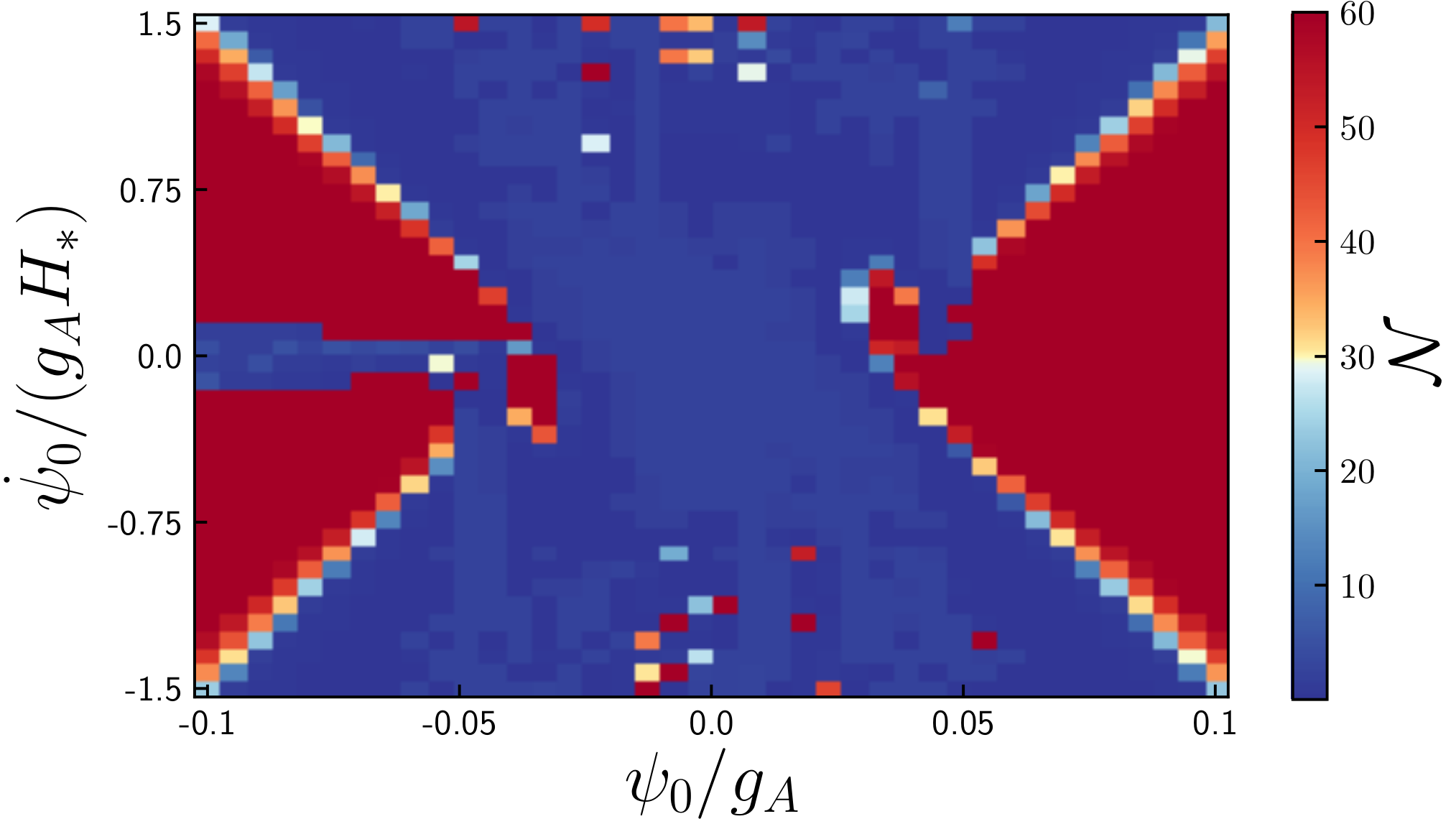
Figure 1 shows the $e$ -folding number,

\displaystyle{\cal N}:=\int_{t_{\rm i}}^{t_{\rm f}}H{\rm d}t,

(29)

calculated for different initial conditions for the gauge field. Here, $t_{\rm i}$ is the initial time and $t_{\rm f}$ is defined as the time at which the energy density of $\chi$ becomes as small as $\rho_{\chi}=10^{-3}M_{\rm Pl}^{2}H_{*}^{2}$ . If this does not occur and inflation lasts for 60 $e$ -folds, we stop the calculation and just set ${\cal N}=60$ . The initial condition for the axion is fixed as

\displaystyle\left[\begin{array}[]{c}\chi_{0}\\ \dot{\chi}_{0}\end{array}\right]=\left[\begin{array}[]{c}\pi f\times 10^{-2}\\ 0\end{array}\right].

For our choice of the parameters, we have $\psi_{\rm min}/g_{A}\simeq 0.07$ , and we can see from Fig. 1 the aforementioned behavior, though the dynamics depends also on the initial value of $\dot{\psi}$ .

Refer to caption — Figure 1: Initial condition dependence of the $e$ -folding number in the flat model. The parameters are given in Table 1.

We now move to the discussion on the case with ${\cal K}>0$ . The evolution of the system would be more complicated due to the various ${\cal K}$ -dependent terms in the basic equations. Now positive spatial curvature does not simply act as effective negative energy density, and hence large positive ${\cal K}$ does not necessarily make the universe collapse. Spatial curvature also modifies the shapes of the effective potentials for $\chi$ and $\psi$ , as seen from Eqs. (17) and (18), and thus affects directly the evolution of these fields.

Let us estimate the effect of spatial curvature in Eq. (19). Assuming that the curvature is large and the kinetic energy of the fields is small enough, Eq. (19) reduces to

\displaystyle 3M_{\rm Pl}^{2}H^{2}

\displaystyle\simeq\frac{3}{2g_{A}^{2}}\frac{{\cal K}^{2}}{a^{4}}-3M_{\rm Pl}^{2}\frac{{\cal K}}{a^{2}}+V,

(34)

and $V\simeq 2\mu^{4}=2M_{\rm Pl}^{2}H_{*}^{2}$ . This can be recast into a dimensionless form as

\displaystyle 1\simeq\frac{1}{2}\left(\frac{H}{g_{A}M_{\rm Pl}}\right)^{2}\left(\frac{{\cal K}}{a^{2}H^{2}}\right)^{2}-\frac{{\cal K}}{a^{2}H^{2}}+\frac{2}{3}\left(\frac{H_{*}}{H}\right)^{2}.

(35)

We consider the case where $H\sim H_{*}$ and ${\cal K}/a^{2}H_{*}^{2}\sim 1$ . It can then be seen that if $g_{A}\sim H_{*}/M_{\rm Pl}$ , the first term in the right-hand side can cancel the second term, supporting the universe against collapse. For larger $g_{A}$ , the first term becomes less important. Note that $g_{A}$ cannot be too small in order for the Friedmann equation to be satisfied in the universe with large spatial curvature.

The above argument can be verified by the numerical result shown in Fig. 2. We run the numerical code for different values of ${\cal K}$ and $g_{A}$ . The initial conditions for the axion and the Hubble parameter are given respectively by Eq. (II.2) and $H_{0}=H_{*}$ , while the initial value of the gauge field is given by $\psi_{0}=0.05\times g_{A}$ . The initial velocity of the gauge field, $\dot{\psi}_{0}$ , is then determined from the Friedmann equation (19), which is different for different $(g_{A},{\cal K})$ . For ${\cal K}$ above a certain value the universe immediately collapses. In Fig. 2 this critical value of ${\cal K}$ is shown as a function of $g_{A}$ . We see that the universe with smaller $g_{A}$ is more stable against the inclusion of positive spatial curvature.

Figure 2: The critical values of

{\cal K}

are shown as black dots, above which the universe immediately collapses.

The initial condition dependence of the $e$ -folding number is also altered by the presence of spatial curvature, as can be seen by comparing Fig. 1 with Fig. 3. We find that, as long as the initial velocity of $\psi$ is small, we have a sufficient duration of the inflationary phase for a wide range of initial conditions $\psi_{0}$ . Note here that the initial conditions plotted in Fig. 3 all satisfy $\psi_{0}^{2}\ll{\cal K}/H_{*}^{2}$ . The typical dynamics of the axion and gauge fields in this case is shown in Fig. 4, which is different from the conventional one in the early stage, but leads in the end to prolonged inflation. In the early stage, the interaction term in the right-hand side of Eq. (17) is maintained even for tiny $\psi_{0}$ for ${\cal O}(1)$ $e$ -folds, because we have $\psi^{2}-{\cal K}/a^{2}\simeq-{\cal K}/a^{2}$ . Then, both fields change their values rapidly at around $H_{*}t\simeq 3$ . This corresponds to the moment at which the right-hand sides of Eqs. (17) and (18) vanishes, $\psi^{2}\simeq{\cal K}/a^{2}$ . After that, $\psi$ -assisted slow-roll inflation occurs at the different side of the potential from the one where the axion field is initially placed. We thus have the unconventional pre-inflationary dynamics leading to successful inflation.

Figure 4: The evolution of the axion and gauge fields with the curvature

\mathcal{K}=0.5H_{*}^{2}

for the initial condition given by Eq. (II.2),

\psi_{0}=10^{-7}M_{\rm Pl}

, and

\dot{\psi}_{0}=-10^{-12}M_{\rm Pl}^{2}

(for which

H_{0}=0.555H_{*}

So far we have considered the case where the axion is the inflaton field. Let us briefly comment on the case where there is another scalar field that plays the role of the inflaton and the axion is a spectator field Dimastrogiovanni_2017. Suppose in this spectator axion-SU(2) model that the inflaton’s potential energy is given by $V_{\rm inf}\sim 2\alpha\mu^{4}$ ( $\alpha>1$ ). This amounts to rescaling $H_{*}$ as $H_{*}\to(1+\alpha)^{1/2}H_{*}$ in Eq. (34). Therefore, for larger inflaton’s contribution (i.e., for larger $\alpha$ ), $g_{A}/H_{*}$ becomes effectively smaller, rendering the universe more stable against the inclusion of positive spatial curvature.

III Multiple vector fields without the non-abelian-specific structure

Let us move to the case of multiple generalized Proca fields Jimenez:2016upj; Emami_2017. In this case, the vector fields do not have the non-abelian-specific structure and hence we cannot use the same ansatz in a spatially curved universe as in the case of the SU(2) gauge field. In this section, we therefore start from reconsidering the metric and vector field ansatz.

The Lagrangian for the model considered in Ref. Emami_2017 contains three vector fields $A_{\mu}^{a}$ ( $a=1,2,3$ ) and is given by

\displaystyle{\cal L}=\mathcal{L}_{2}+\mathcal{L}_{4},

(36)

with

	$\displaystyle\mathcal{L}_{2}$	$\displaystyle=G_{2}\left(X,Y,Z,W_{1},W_{2},W_{3}\right),$		(37)
	$\displaystyle\mathcal{L}_{4}$	$\displaystyle=G_{4}(X)R+G_{4,X}\left[\nabla_{\mu}A^{\mu}_{a}\nabla^{\nu}A_{\nu}^{a}-\nabla_{\mu}A_{\nu}^{a}\nabla^{\nu}A^{\mu}_{a}\right],$		(38)

where

		$\displaystyle X:=-\frac{1}{2}A_{\mu}^{a}A^{\mu}_{a},\quad Y:=-\frac{1}{4}F_{\mu\nu}^{a}F^{\mu\nu}_{a},$
		$\displaystyle Z:=-\frac{1}{4}F_{\mu\nu}^{a}\widetilde{F}^{\mu\nu}_{a},\quad W_{1}:=A_{\mu}^{a}A^{\nu}_{a}F^{\mu\rho}_{b}F_{\nu\rho}^{b},$
		$\displaystyle W_{2}:=A_{\mu}^{a}A^{\nu}_{b}F^{\mu\rho}_{a}F_{\nu\rho}^{b},\quad W_{3}:=A_{\mu}^{a}A^{\nu}_{b}F^{\mu\rho}_{b}F_{\nu\rho}^{a},$		(39)

and note that in the present case

\displaystyle F_{\mu\nu}^{a}:=\partial_{\mu}A_{\nu}^{a}-\partial_{\nu}A_{\mu}^{a}.

(40)

To explore the configuration of the vector fields, we first note that the metric of a closed universe can be written using the left-invariant 1-forms as

\displaystyle\mathrm{d}s^{2}=-N^{2}(t)\mathrm{d}t^{2}+\frac{a^{2}(t)}{4}\delta_{ab}\omega^{a}\omega^{b},

(41)

where

$\displaystyle\omega^{1}$	$\displaystyle=-\sin\left(\sqrt{\mathcal{K}}x^{3}\right)\mathrm{d}x^{1}+\sin\left(\sqrt{\mathcal{K}}x^{1}\right)\cos\left(\sqrt{\mathcal{K}}x^{3}\right)\mathrm{d}x^{2},$	(42)
$\displaystyle\omega^{2}$	$\displaystyle=\cos\left(\sqrt{\mathcal{K}}x^{3}\right)\mathrm{d}x^{1}+\sin\left(\sqrt{\mathcal{K}}x^{1}\right)\sin\left(\sqrt{\mathcal{K}}x^{3}\right)\mathrm{d}x^{2},$	(43)
$\displaystyle\omega^{3}$	$\displaystyle=\cos\left(\sqrt{\mathcal{K}}x^{1}\right)\mathrm{d}x^{2}+\mathrm{d}x^{3}.$	(44)

Notice that this expression can be used only for a closed universe. We then assume that the vector fields take the form²² 2 In Appendix A, we show that the same ansatz can also be used for the SU(2) gauge field, reproducing the same result as in Sec. II up to field redefinition.

\displaystyle A_{0}^{a}=0,\quad A_{i}^{a}\mathrm{d}x^{i}=\frac{a}{2}\psi(t)\omega^{a},

(45)

where we set $A_{0}^{a}=0$ because it is indeed a trivial solution. Under the above ansatz we have

$\displaystyle X$	$\displaystyle=-\frac{3}{2}\psi^{2},$	(46)
$\displaystyle Y$	$\displaystyle=\frac{3}{2}\left[\frac{1}{N^{2}}\left(\dot{\psi}+\frac{\dot{a}}{a}\psi\right)^{2}-\frac{4\mathcal{K}}{a^{2}}\psi^{2}\right],$	(47)
$\displaystyle Z$	$\displaystyle=\frac{6}{N}\psi\left(\dot{\psi}+\frac{\dot{a}}{a}\psi\right)\frac{\sqrt{\mathcal{K}}}{a},$	(48)
$\displaystyle W_{1}$	$\displaystyle=-3\psi^{2}\left[\frac{1}{N^{2}}\left(\dot{\psi}+\frac{\dot{a}}{a}\psi\right)^{2}-\frac{8\mathcal{K}}{a^{2}}\psi^{2}\right],$	(49)
$\displaystyle W_{2}$	$\displaystyle=-\frac{9}{N^{2}}\psi^{2}\left(\dot{\psi}+\frac{\dot{a}}{a}\psi\right)^{2},$	(50)
$\displaystyle W_{3}$	$\displaystyle=-3\psi^{2}\left[\frac{1}{N^{2}}\left(\dot{\psi}+\frac{\dot{a}}{a}\psi\right)^{2}+\frac{8\mathcal{K}}{a^{2}}\psi^{2}\right],$	(51)

and

\displaystyle\nabla_{\mu}A^{\mu}_{a}\nabla^{\nu}A_{\nu}^{a}-\nabla_{\mu}A_{\nu}^{a}\nabla^{\nu}A^{\mu}_{a}=-\frac{6}{N^{2}}\frac{\dot{a}}{a}\dot{\psi}\psi+\frac{6\mathcal{K}}{a^{2}}\psi^{2}.

(52)

We see that each piece in the Lagrangian depends only on $t$ , and therefore the above assumed configuration of the vector fields is consistent with a closed universe. In contrast to the spatially flat case Emami_2017, $Z$ is no longer vanishing in a positively curved universe.

Let us present two applications of the our result. The first example is the vector inflation model proposed in Ref. Golovnev:2008cf, whose Lagrangian is given by

\displaystyle{\cal L}=\left(\frac{M_{\rm Pl}^{2}}{2}-\xi X\right)R+Y+m^{2}X,

(53)

where $\xi$ and $m$ are constants, and below we will set $\xi=1/6$ . Strictly speaking, this does not belong to the multiple generalized Proca theory, as the Lagrangian (53) is obtained by omitting $G_{4,X}$ by hand Emami_2017. Nevertheless, one can use the ansatz (45) to analyze the dynamic of the vector inflation model of Golovnev:2008cf with ${\cal K}>0$ , since, as seen from Eqs. (46) and (47), both $X$ and $Y$ are dependent only on $t$ . Our field equations are given by

		$\displaystyle\ddot{\psi}+3H\dot{\psi}+\left(m^{2}+\frac{3\mathcal{K}}{a^{2}}\right)\psi=0,$		(54)
		$\displaystyle 3M_{\rm Pl}^{2}\left(H^{2}+\frac{\mathcal{K}}{a^{2}}\right)=\frac{3}{2}\left(\dot{\psi}^{2}+m^{2}\psi^{2}\right)+\frac{9\mathcal{K}}{2a^{2}}\psi^{2},$		(55)
		$\displaystyle 2M_{\rm Pl}^{2}\left(\dot{H}-\frac{\mathcal{K}}{a^{2}}\right)=-3\dot{\psi}^{2}-\frac{3\mathcal{K}}{a^{2}}\psi^{2}.$		(56)

Open and closed FLRW models in the theory (53) have been studied earlier in Ref. Chiba:2008eh. Our result disagrees with that of Ref. Chiba:2008eh; it seems that the consistent ansatz for the vector fields has not been employed in Chiba:2008eh. The sign of the vector-field-induced curvature terms in Eqs. (54)–(56) is opposite compared to the result of Chiba:2008eh, and accordingly the dynamics should be qualitatively different as compared to Chiba:2008eh.

The second example is the model with a triplet of vector fields coupled to a scalar field. Obviously, the ansatz (45) can be used in such a case as well. For example, the model studied in Ref. Gorji_2020 is described by the Lagrangian

\displaystyle\mathcal{L}=\frac{M_{\rm Pl}^{2}}{2}R-\frac{1}{2}(\partial\phi)^{2}-V(\phi)+f^{2}(\phi)\left(Y+\theta Z\right),

(57)

where $\theta$ is a constant. In this case, the vector fields have the U(1) $\times$ U(1) $\times$ U(1) symmetry. (One may thus use this symmetry to eliminate $A_{0}^{a}$ .) Let us investigate the cosmological background dynamics of this model in more detail. The field equations are given by

		$\displaystyle\ddot{\phi}+3H\dot{\phi}+V^{\prime}-3ff^{\prime}(\dot{\psi}+H\psi)^{2}$
		$\displaystyle+12ff^{\prime}\psi\left[\frac{{\cal K}}{a^{2}}\psi+\theta\frac{\sqrt{\cal K}}{a}(\dot{\psi}+H\psi)\right]=0,$		(58)
		$\displaystyle\ddot{\psi}+3H\dot{\psi}+\left(\dot{H}+2H^{2}\right)\psi+\frac{2f^{\prime}}{f}\dot{\phi}\left(\dot{\psi}+H\psi\right)$
		$\displaystyle+4\psi\left(\frac{\mathcal{K}}{a^{2}}-\theta\frac{\sqrt{\mathcal{K}}}{a}\frac{f^{\prime}}{f}\dot{\phi}\right)=0,$		(59)
		$\displaystyle 3M_{\rm Pl}^{2}\left(H^{2}+\frac{\mathcal{K}}{a^{2}}\right)=\frac{\dot{\phi}^{2}}{2}+V+\frac{6\mathcal{K}}{a^{2}}f^{2}\psi^{2}$
		$\displaystyle\qquad\qquad\qquad\qquad\quad+\frac{3}{2}f^{2}\left(\dot{\psi}+H\psi\right)^{2},$		(60)
		$\displaystyle M_{\rm Pl}^{2}\left(\dot{H}-\frac{\cal K}{a^{2}}\right)=-\frac{\dot{\phi}^{2}}{2}-\frac{4\mathcal{K}}{a^{2}}f^{2}\psi^{2}-f^{2}\left(\dot{\psi}+H\psi\right)^{2},$		(61)

where a prime stands for differentiation with respect to $\phi$ . In the following, we will consider the particular form of the potential and the coupling function given by

\displaystyle V=\frac{1}{2}m^{2}\phi^{2},\quad f=f_{*}\exp\left[\frac{2M_{\rm Pl}^{-2}}{1-I}\int^{\phi}_{\phi_{*}}\frac{V(\widetilde{\phi})}{V^{\prime}(\widetilde{\phi})}{\rm d}\widetilde{\phi}\right],

(62)

where $m$ , $I$ , $f_{*}$ , and $\phi_{*}$ are constants. This particular case was also studied in Ref. Gorji_2020 and shown to admit an inflationary attractor solution with nonvanishing vector fields Firouzjahi:2018wlp.

For a fixed value of ${\cal K}/a_{0}^{2}H_{0}^{2}$ , we numerically solve the field equations to see whether the universe continues to expand toward the inflationary attractor or stops expanding at a certain moment and eventually collapses. Let us first switch off the vector fields by setting $f_{*}=0$ and consider the case where ${\cal K}/a_{0}^{2}H_{0}^{2}=7.5$ at the initial moment. We take $m=10^{-2}M_{\rm Pl}$ . It is easy to see that for the initial condition $(\phi_{0},\dot{\phi}_{0})=(10M_{\rm Pl},-0.1M_{\rm Pl}^{2})$ the universe stops expanding within one $e$ -fold and then collapses. We then include the vector fields with $f(\phi_{0})=0.1$ , $I=0.1$ , and $\theta=0$ . For the initial condition $(\phi_{0},\dot{\phi}_{0},\psi_{0},\dot{\psi}_{0})=(10M_{\rm Pl},-0.1M_{\rm Pl}^{2},M_{\rm Pl},0)$ , we find that the universe expands toward the inflationary attractor rather than collapses even in the presence of such a large spatial curvature at the initial moment. This implies that the triplet of vector fields can save the universe from collapsing.

Figure 5 shows the numerical results for different initial conditions satisfying $(1/2)\dot{\phi}_{0}^{2}+V(\phi_{0})=10^{-2}M_{\rm Pl}^{4}$ , with $(\psi_{0},\dot{\psi}_{0})=(M_{\rm Pl},0)$ . The parameters are the same as above: ${\cal K}/a_{0}^{2}H_{0}^{2}=7.5$ , $m=10^{-2}M_{\rm Pl}$ , $I=0.1$ , and $\theta=0$ . For each calculation we introduce $f_{*}$ and $\phi_{*}$ so that $f(\phi_{0})=0.1$ , We see that the fraction of initial conditions leading to successful inflation indeed increases with the help of the vector fields, though the effect is not so significant.

Figure 5: The circles represent the initial conditions that result in inflation both with and without the vector fields, while for the initial conditions represented by the crosses the universe immediately collapses in any case. For the initial conditions represented by the triangles, the universe without the vector fields collapses, but with the help of the vector fields it avoids to do so, leading to successful inflation. No initial conditions are found for which the vector fields hinder inflation. Due to the symmetry only the cases with

\phi_{0}>0

are shown.

In Fig. 6, we present typical phase space trajectories in the presence of the vector fields. It can be seen that the dynamics of the inflaton shows an oscillatory nature during the early stage in which the effect of the spatial curvature is large. This pre-inflationary dynamics is caused by the interplay among the inflaton, the vector fields, and ${\cal K}$ . In this phase, the inflaton equation of motion (58) is given approximately by

\displaystyle\ddot{\phi}+3H\dot{\phi}\simeq 3ff^{\prime}\left(\dot{\psi}^{2}-\frac{4{\cal K}}{a^{2}}\psi^{2}\right),

(63)

and the sign of the right-hand side flips several times because $\psi$ oscillates around zero, yielding the oscillatory dynamics as shown in Fig. 6.

Figure 6: Trajectories of the inflaton in the phase space. Black points represent the initial conditions.

IV Conclusions and discussion

In this paper, we have studied the dynamics of a homogeneous, isotropic, and positively curved universe in the presence of the SU(2) gauge field or a triplet of mutually orthogonal vector fields, and obtained the following results.

•

We have obtained the consistent ansatz for a triplet of the generalized Proca fields in a closed universe, which corrects the previous analysis of a certain vector-field model of inflation in a curved universe. Our ansatz can also be used to the SU(2) gauge field and reproduces the known result up to field redefinition.
•

In addition to the usual curvature terms in the cosmological equations, new curvature-dependent terms appear through the vector fields. In the cases of axion-SU(2) inflation Adshead:2012kp and inflation with the vector fields having U(1) $\times$ U(1) $\times$ U(1) symmetry Gorji_2020, we have found that the vector fields support the closed universe against collapse, though the effect is not so significant.
•

In both models we have found nontrivial pre-inflationary dynamics caused by spatial curvature.

Let us discuss a possible extension of the present study. It is easy to see that the ansatz we have introduced in Sec. III can be generalized straightforwardly to include spatial anisotropies

		$\displaystyle{\rm d}s^{2}=-N^{2}(t){\rm d}t^{2}+h_{ab}\omega^{a}\omega^{b},$		(64)
		$\displaystyle h_{ab}=\frac{a^{2}}{4}\times{\rm diag}(e^{-4\sigma_{+}},e^{2\sigma_{+}+2\sqrt{3}\sigma_{-}},e^{2\sigma_{+}-2\sqrt{3}\sigma_{-}}),$		(65)
		$\displaystyle A_{i}^{a}{\rm d}x^{i}=\sqrt{h_{aa}}\psi_{a}\omega^{a}\quad(\text{no summation over }a),$		(66)
		$\displaystyle\psi_{a}=\psi(t)\times(e^{-2\beta_{+}},e^{\beta_{+}+\sqrt{3}\beta_{-}},e^{\beta_{+}-\sqrt{3}\beta_{-}}),$		(67)

where $\sigma_{\pm}=\sigma_{\pm}(t)$ and $\beta_{\pm}=\beta_{\pm}(t)$ characterize anisotropies. It would therefore be interesting to explore the Bianchi type-IX dynamics in the presence of mutually orthogonal vector fields, which is left for further study.

Acknowledgements.

TK was partially supported by JSPS KAKENHI Grants No. JP20H04745 and No. JP20K03936.

Appendix A Ansatz (45) applied to the SU(2) gauge field

In this Appendix let us confirm that the ansatz (45) can also be used for the SU(2) gauge field and the same result as in Sec. II is reproduced up to field redefinition (for ${\cal K}>0$ ). Using Eqs. (41) and (45) we find

	$\displaystyle F_{\mu\nu}^{a}F_{a}^{\mu\nu}$	$\displaystyle=-6\left[\frac{1}{N^{2}}\left(\dot{\psi}+\frac{\dot{a}}{a}\psi\right)^{2}-\psi^{2}\left(g_{A}\psi+\frac{2\sqrt{{\cal K}}}{a}\right)^{2}\right],$		(68)
	$\displaystyle\widetilde{F}^{a}_{\mu\nu}F_{a}^{\mu\nu}$	$\displaystyle=-\frac{12}{N}\left(\dot{\psi}+\frac{\dot{a}}{a}\psi\right)\psi\left(g_{A}\psi+\frac{2\sqrt{{\cal K}}}{a}\right).$		(69)

These are apparently different from Eqs. (15) and (16). It is easy, however, to see that in terms of the new variable

\displaystyle\psi_{\rm new}:=-g_{A}\psi-\frac{\sqrt{{\cal K}}}{a},

(70)

Eqs. (68) and (69) coincide with Eqs. (15) and (16), respectively.

In the context of FLRW cosmologies in the presence of gauge sectors, the same ansatz for the gauge field has been studied in Ref. Moniz:1990hf and its application can be found in Ref. VargasMoniz:2002gj

References

(1) A. A. Starobinsky, A New Type of Isotropic Cosmological Models Without Singularity, Phys. Lett. B 91 (1980) 99.
(2) A. H. Guth, Inflationary universe: A possible solution to the horizon and flatness problems, Phys. Rev. D 23 (1981) 347.
(3) K. Sato, First Order Phase Transition of a Vacuum and Expansion of the Universe, Mon. Not. Roy. Astron. Soc. 195 (1981) 467.
(4) R. M. Wald, Asymptotic behavior of homogeneous cosmological models in the presence of a positive cosmological constant, Phys. Rev. D 28 (1983) 2118.
(5) V. A. Belinsky, H. Ishihara, I. M. Khalatnikov and H. Sato, On the Degree of Generality of Inflation in Friedman Cosmological Models With a Massive Scalar Field, Prog. Theor. Phys. 79 (1988) 676.
(6) V. A. Belinsky, I. M. Khalatnikov, L. P. Grishchuk and Y. B. Zeldovich, INFLATIONARY STAGES IN COSMOLOGICAL MODELS WITH A SCALAR FIELD, Phys. Lett. B 155 (1985) 232.
(7) A. Albrecht, R. H. Brandenberger and R. Matzner, Numerical Analysis of Inflation, Phys. Rev. D 32 (1985) 1280.
(8) H. Kurki-Suonio, R. A. Matzner, J. Centrella and J. R. Wilson, Inflation From Inhomogeneous Initial Data in a One-dimensional Back Reacting Cosmology, Phys. Rev. D 35 (1987) 435.
(9) D. S. Goldwirth and T. Piran, Spherical Inhomogeneous Cosmologies and Inflation. 1. Numerical Methods, Phys. Rev. D 40 (1989) 3263.
(10) D. S. Goldwirth and T. Piran, Inhomogeneity and the Onset of Inflation, Phys. Rev. Lett. 64 (1990) 2852.
(11) H. Kurki-Suonio, P. Laguna and R. A. Matzner, Inhomogeneous inflation: Numerical evolution, Phys. Rev. D 48 (1993) 3611 [astro-ph/9306009].
(12) W. E. East, M. Kleban, A. Linde and L. Senatore, Beginning inflation in an inhomogeneous universe, JCAP 09 (2016) 010 [1511.05143].
(13) R. Brandenberger, Initial conditions for inflation — A short review, Int. J. Mod. Phys. D 26 (2017) 1740002 [1601.01918].
(14) K. Clough, E. A. Lim, B. S. DiNunno, W. Fischler, R. Flauger and S. Paban, Robustness of Inflation to Inhomogeneous Initial Conditions, JCAP 09 (2017) 025 [1608.04408].
(15) M. C. D. Marsh, J. D. Barrow and C. Ganguly, Inhomogeneous Initial Data and Small-Field Inflation, JCAP 05 (2018) 026 [1803.00625].
(16) J. C. Aurrekoetxea, K. Clough, R. Flauger and E. A. Lim, The Effects of Potential Shape on Inhomogeneous Inflation, JCAP 05 (2020) 030 [1910.12547].
(17) R. Easther, L. C. Price and J. Rasero, Inflating an Inhomogeneous Universe, JCAP 08 (2014) 041 [1406.2869].
(18) A. Golovnev, V. Mukhanov and V. Vanchurin, Vector Inflation, JCAP 06 (2008) 009 [0802.2068].
(19) P. Adshead and M. Wyman, Chromo-Natural Inflation: Natural inflation on a steep potential with classical non-Abelian gauge fields, Phys. Rev. Lett. 108 (2012) 261302 [1202.2366].
(20) A. Maleknejad, M. M. Sheikh-Jabbari and J. Soda, Gauge Fields and Inflation, Phys. Rept. 528 (2013) 161 [1212.2921].
(21) J. Beltran Jimenez and L. Heisenberg, Generalized multi-Proca fields, Phys. Lett. B 770 (2017) 16 [1610.08960].
(22) E. Allys, P. Peter and Y. Rodriguez, Generalized SU(2) Proca Theory, Phys. Rev. D 94 (2016) 084041 [1609.05870].
(23) R. Emami, S. Mukohyama, R. Namba and Y. li Zhang, Stable solutions of inflation driven by vector fields, JCAP 03 (2017) 058 [1612.09581].
(24) A. Gallego Cadavid, Y. Rodriguez and L. G. Gómez, Generalized SU(2) Proca theory reconstructed and beyond, Phys. Rev. D 102 (2020) 104066 [2009.03241].
(25) M. A. Gorji, S. A. H. Mansoori and H. Firouzjahi, Inflation with multiple vector fields and non-gaussianities, JCAP 11 (2020) 041 [2008.08195].
(26) C. Armendariz-Picon, Could dark energy be vector-like?, JCAP 07 (2004) 007 [astro-ph/0405267].
(27) Y. Rodríguez and A. A. Navarro, Non-Abelian $S$ -term dark energy and inflation, Phys. Dark Univ. 19 (2018) 129 [1711.01935].
(28) J. Beltrán Jiménez and L. Heisenberg, Non-trivial gravitational waves and structure formation phenomenology from dark energy, JCAP 09 (2018) 035 [1806.01753].
(29) M. Álvarez, J. B. Orjuela-Quintana, Y. Rodriguez and C. A. Valenzuela-Toledo, Einstein Yang–Mills Higgs dark energy revisited, Class. Quant. Grav. 36 (2019) 195004 [1901.04624].
(30) A. Maleknejad and M. M. Sheikh-Jabbari, Gauge-flation: Inflation From Non-Abelian Gauge Fields, Phys. Lett. B 723 (2013) 224 [1102.1513].
(31) A. Maleknejad and M. M. Sheikh-Jabbari, Non-Abelian Gauge Field Inflation, Phys. Rev. D 84 (2011) 043515 [1102.1932].
(32) A. Maleknejad, M. M. Sheikh-Jabbari and J. Soda, Gauge-flation and Cosmic No-Hair Conjecture, JCAP 01 (2012) 016 [1109.5573].
(33) C. M. Nieto and Y. Rodriguez, Massive Gauge-flation, Mod. Phys. Lett. A 31 (2016) 1640005 [1602.07197].
(34) P. Adshead, E. Martinec, E. I. Sfakianakis and M. Wyman, Higgsed Chromo-Natural Inflation, JHEP 12 (2016) 137 [1609.04025].
(35) P. Adshead and E. I. Sfakianakis, Higgsed Gauge-flation, JHEP 08 (2017) 130 [1705.03024].
(36) L. G. Gómez and Y. Rodríguez, Stability Conditions in the Generalized SU(2) Proca Theory, Phys. Rev. D 100 (2019) 084048 [1907.07961].
(37) A. Guarnizo, J. B. Orjuela-Quintana and C. A. Valenzuela-Toledo, Dynamical analysis of cosmological models with non-Abelian gauge vector fields, Phys. Rev. D 102 (2020) 083507 [2007.12964].
(38) L. G. Gomez and Y. Rodriguez, Coupled Multi-Proca Vector Dark Energy, Phys. Dark Univ. 31 (2021) 100759 [2004.06466].
(39) M. C. Bento, O. Bertolami, P. V. Moniz, J. M. Mourao and P. M. Sa, On the cosmology of massive vector fields with SO(3) global symmetry, Class. Quant. Grav. 10 (1993) 285 [gr-qc/9302034].
(40) K.-i. Maeda and K. Yamamoto, Inflationary Dynamics with a Non-Abelian Gauge Field, Phys. Rev. D 87 (2013) 023528 [1210.4054].
(41) K. Yamamoto, Primordial Fluctuations from Inflation with a Triad of Background Gauge Fields, Phys. Rev. D 85 (2012) 123504 [1203.1071].
(42) H. Funakoshi and K. Yamamoto, Primordial bispectrum from inflation with background gauge fields, Class. Quant. Grav. 30 (2013) 135002 [1212.2615].
(43) A. Maleknejad and E. Erfani, Chromo-Natural Model in Anisotropic Background, JCAP 03 (2014) 016 [1311.3361].
(44) I. Wolfson, A. Maleknejad and E. Komatsu, How attractive is the isotropic attractor solution of axion-SU(2) inflation?, JCAP 09 (2020) 047 [2003.01617].
(45) I. Wolfson, A. Maleknejad, T. Murata, E. Komatsu and T. Kobayashi, The isotropic attractor solution of axion-SU(2) inflation: Universal isotropization in Bianchi type-I geometory, 2105.06259.
(46) K.-i. Maeda and K. Yamamoto, Stability analysis of inflation with an SU(2) gauge field, JCAP 12 (2013) 018 [1310.6916].
(47) Y. Hosotani, Exact Solution to the Einstein Yang-Mills Equation, Phys. Lett. B 147 (1984) 44.
(48) D. Galtsov and M. Volkov, Yang-Mills cosmology: Cold matter for a hot universe, Phys. Lett. B 256 (1991) 17.
(49) D. V. Gal’tsov, Non-Abelian condensates as alternative for dark energy, in 43rd Rencontres de Moriond on QCD and High Energy Interactions, 12, 2008, 0901.0115.
(50) M. A. Gorji, S. Mukohyama and H. Firouzjahi, Cosmology in Mimetic SU(2) Gauge Theory, JCAP 05 (2019) 019 [1903.04845].
(51) E. Dimastrogiovanni, M. Fasiello and T. Fujita, Primordial gravitational waves from axion-gauge fields dynamics, JCAP 01 (2017) 019 [1608.04216].
(52) T. Chiba, Initial Conditions for Vector Inflation, JCAP 08 (2008) 004 [0805.4660].
(53) H. Firouzjahi, M. A. Gorji, S. A. Hosseini Mansoori, A. Karami and T. Rostami, Charged Vector Inflation, Phys. Rev. D 100 (2019) 043530 [1812.07464].
(54) P. V. Moniz and J. M. Mourao, Homogeneous and isotropic closed cosmologies with a gauge sector, Class. Quant. Grav. 8 (1991) 1815.
(55) P. Vargas Moniz, FRW wormhole instantons in the nonAbelian Born-Infeld theory, Phys. Rev. D 66 (2002) 064012.