Inferring kilonova population properties with a hierarchical Bayesian framework I : Non-detection methodology and single-event analysesipython (Pérez & Granger 2007), jupyter (Kluyver et al. 2016), matplotlib (Hunter 2007), python (Van Rossum & Drake 2009), NumPy (Harris et al. 2020), scikit-learn (Pedregosa et al. 2011), scipy (Virtanen et al. 2020)Facilities: LIGO, ZTF/PO:1.2m
Abstract
We present nimbus: a hierarchical Bayesian framework to infer the intrinsic luminosity parameters of kilonovae (KNe) associated with gravitational-wave (GW) events, based purely on non-detections. This framework makes use of GW 3-D distance information and electromagnetic upper limits from multiple surveys for multiple events, and self-consistently accounts for finite sky-coverage and probability of astrophysical origin. The framework is agnostic to the brightness evolution assumed and can account for multiple electromagnetic passbands simultaneously. Our analyses highlight the importance of accounting for model selection effects, especially in the context of non-detections. We show our methodology using a simple, two-parameter linear brightness model, taking the follow-up of GW190425 with the Zwicky Transient Facility (ZTF) as a single-event test case for two different prior choices of model parameters – (i) uniform/uninformative priors and (ii) astrophysical priors based on surrogate models of Monte Carlo radiative transfer simulations of KNe. We present results under the assumption that the KN is within the searched region to demonstrate functionality and the importance of prior choice. Our results show consistency with simsurvey – an astronomical survey simulation tool used previously in the literature to constrain the population of KNe. While our results based on uniform priors strongly constrain the parameter space, those based on astrophysical priors are largely uninformative, highlighting the need for deeper constraints. Future studies with multiple events having electromagnetic follow-up from multiple surveys should make it possible to constrain the KN population further.
I Introduction
Mergers of neutron stars and neutron star-black hole binaries (BNS and NSBH) present unique opportunities to probe multi-messenger astrophysics (Metzger 2019, e.g.,). While they are among the best sources of gravitational-wave (GW) emission detectable by GW observatories (Abbott et al. 2019; Abbott et al. 2020) such as Advanced LIGO and Advanced Virgo (Aasi et al. 2015; Acernese et al. 2015), their potential detection in the electro-magnetic (EM) spectrum by surveys around the world represents one of the most challenging searches for astrophysical transients. During the merger, significant amounts of neutron-star (NS) matter are ejected at sub-relativistic speeds due to either tidal or hydrodynamical forces; the radioactive decay of -process elements synthesized in the neutron-rich merger ejecta powers a thermal ultraviolet, optical and near infrared transient, often referred to as a kilonova (KN) (Li & Paczyński 1998; Rosswog 2005; Metzger et al. 2010; Tanaka & Hotokezaka 2013). Despite their color- and luminosity-evolution being viewing-angle dependent (Kasen et al. 2015; Bulla 2019; Kawaguchi et al. 2020; Korobkin et al. 2020; Zhu et al. 2021), their (largely) isotropic emission makes KNe one of the promising targets for EM counterpart follow-up observations (Roberts et al. 2011). However, they can be short-lived, faint, and peak in the infrared, making detection difficult (Kasen et al. 2015; Tanaka 2016; Barnes et al. 2016; Metzger 2019; Nakar 2019).
From an observational standpoint, the GW detection of the BNS merger GW170817 (Abbott et al. 2017b) provided the first, and only, multi-messenger follow-up of a GW event to yield an associated KN (AT2017gfo) to date (Abbott et al. 2017). Observations were recorded in the ultraviolet, optical and near-infrared (Andreoni et al. 2017; Chornock et al. 2017; Coulter et al. 2017; Cowperthwaite et al. 2017; Drout et al. 2017; Evans et al. 2017; Kasliwal et al. 2017; Kasliwal et al. 2019b; Kilpatrick et al. 2017; Lipunov et al. 2017; McCully et al. 2017; Nicholl et al. 2017; Shappee et al. 2017; Soares-Santos et al. 2017; Pian et al. 2017; Smartt et al. 2017; Tanvir et al. 2017; Utsumi et al. 2017). These observations have highlighted the ability to test models of KNe and provide constraints on the ejecta mass and velocity (Abbott et al. 2017a; Cowperthwaite et al. 2017; Perego et al. 2017; Pian et al. 2017; Smartt et al. 2017; Tanaka et al. 2017; Waxman et al. 2018; Coughlin et al. 2019a; Kawaguchi et al. 2020; Heinzel et al. 2021; Raaijmakers et al. 2021), -process elemental abundances (Côté et al. 2018; Hotokezaka et al. 2018; Radice et al. 2018; Tanaka et al. 2018; Hotokezaka & Nakar 2020; Siegel 2019), the NS equation of state (Foucart et al. 2018; Coughlin et al. 2018a; Radice & Dai 2019; Hinderer et al. 2019; Breschi et al. 2021; Nicholl et al. 2021) and Hubble Constant (Hotokezaka et al. 2019; Dietrich et al. 2020; Dhawan et al. 2020).
There are a plethora of studies in the literature that model the luminosity evolution of KNe (Kasen et al. 2017; Coughlin et al. 2018a; Wollaeger et al. 2018; Bulla 2019; Kawaguchi et al. 2020; also see references in Metzger 2019). Despite the detection of the KN from GW170817, there are significant uncertainties in the model parameter space (Barnes et al. 2016; Rosswog et al. 2017; Zhu et al. 2018; Kasliwal et al. 2019b; Wu et al. 2019; Heinzel et al. 2021). These uncertainties primarily stem from the range of ejecta masses expected from such mergers and the content of nuclear matter assumed in the models (Barnes et al. 2020; Foucart et al. 2021; Kullmann et al. 2021; Just et al. 2021). While uncertainties in the mass ejected from BNS systems have been shown to be driven mostly by the total mass and mass ratio of the system (Bauswein et al. 2013; Hotokezaka et al. 2013; Köppel et al. 2019; Kiuchi et al. 2019), those in models for NSBH systems are influenced by the mass ratio, BH spin and NS radius (Etienne et al. 2009; Kyutoku et al. 2015; Kawaguchi et al. 2016; Foucart et al. 2018; Zhu et al. 2020).
The third observing run of Advanced LIGO and Virgo (O311 1 https://gracedb.ligo.org/superevents/public/O3/), which lasted 11 months, yielded a total of 15 publicly announced NSBH and BNS candidates. Several teams, including Global Relay of Observatories Watching Transients Happen (GROWTH; Kasliwal et al. 2020), Electromagnetic counterparts of gravitational wave sources at the Very Large Telescope (ENGRAVE; Levan 2020), Global Rapid Advanced Network Devoted to the Multi-messenger Addicts (GRANDMA; Antier et al. 2020), Gravitational-wave Optical Transient Observer (GOTO; Gompertz et al. 2020), All Sky Automated Survey for SuperNovae (ASAS-SN; deJaeger2021_ASASN), Asteroid Terrestrial Last Alert System (ATLAS; Tonry et al. 2018), Panoramic Survey Telescope and Rapid Response System (Pan-STARRS; Chambers et al. 2016), MASTER-Net (Lipunov et al. 2017), Dark Energy Survey Gravitational Wave Collaboration (DES-GW; Soares-Santos et al. 2017) and Japanese collaboration for Gravitational wave ElectroMagnetic follow-up (J-GEM; Sasada et al. 2021) conducted wide-field searches within the skymaps of BNS and NSBH candidates and pursued follow-up of interesting transient candidates found therein, but no plausible EM counterparts were found (e.g., Coughlin et al. 2019d).
Nevertheless, the apparent dearth of counterparts during all of O3 can illuminate our understanding of the intrinsic properties of KNe. On an individual GW event basis, observational upper limits can be used to constrain the KN emission from a potentially associated counterpart and infer properties of the binary (Hosseinzadeh et al. 2019; Andreoni et al. 2020; Anand et al. 2020; Morgan et al. 2020). Other works, e.g., Coughlin et al. 2019d; Lundquist et al. 2019b; Gompertz et al. 2020; Antier et al. 2020; Kasliwal et al. 2020, have demonstrated ways to synthesize survey observations for a suite of GW events to constrain the KN population as a whole. In particular, Kasliwal et al. 2020 formulated a method for constraining the luminosity function of the KN population. Assuming a non-uniform distribution of KN initial luminosities between 10 and 20 absolute magnitude, their findings suggest that no more than 57% (89%) of KNe could be brighter than 16.6 mag assuming flat (fading at 1 mag day-1) evolution (Kasliwal et al. 2020).
In this paper, we present nimbus(Mohite 2021): a hierarchical Bayesian framework to infer the intrinsic luminosity parameters of the population of KNe associated with GW events, based purely on non-detections. Key features of this framework include the simultaneous use of probabilistic source distance information from GW observations and corresponding upper limits from EM surveys, accounting for the fraction of the skymap searched by a given survey for each event, self-consistent inclusion of the probability of a GW event being of astrophysical origin () and the ability to model multi-band luminosity evolution. The framework is agnostic to the specific luminosity model used and thus can be used to constrain a wide variety of models in the literature.
As a first example and proof of concept, we demonstrate realistic constraints possible on the KN emission from the past follow-up of the event GW190425 (Abbott et al. 2020) conducted with the Zwicky Transient Facility (ZTF) (Coughlin et al. 2019c). ZTF is an optical time-domain survey, consisting of a CCD camera with a 47 deg2 field-of-view installed on the 48-inch Samuel Oschin Schmidt Telescope at the Palomar Observatory. Scanning the sky at an areal survey speed of 3750 square degrees per hour in three custom filters, ZTF-, ZTF-, ZTF-; it reaches a median depth of 20.4 mag in 30 s exposures in its nominal nightly survey but can also conduct deeper target-of-opportunity followup of external events (Coughlin et al. 2019b); for a comprehensive review of the ZTF instrument, software, and survey see Bellm et al. 2019; Masci et al. 2019; Graham et al. 2019; Dekany et al. 2020.
Among the 13 events searched by ZTF in Advanced LIGO’s third observing run (Kasliwal et al. 2020) that could have a probable EM counterpart, based on the probability of the system containing a NS i.e. p(BNS) or p(NSBH), GW190425 is so far the only significant binary merger event confirmed by LIGO and Virgo (Abbott et al. 2020) to likely be a BNS based on the posterior inference of its masses; therefore, our analysis herein focuses on this event alone. GW190425 was located at a distance of 159 Mpc and its final 90% credible localization spanned 8284 deg2 (Abbott et al. 2020). For GW190425, ZTF observed 8000 deg2, corresponding to 45% probability of the initial BAYESTAR skymap (Singer & Price 2016) which reduced to 21% integrated probability within the 90% credible region of the LALInference skymap (Veitch et al. 2015) and attained a median depth of m21 mag in - and -bands (Coughlin et al. 2019b). For the purpose of this analysis, we consider ZTF areal coverage within the entire LALInference skymap, which corresponds to 32% probability. No KN was identified in the observed region of this event by ZTF or other optical telescopes (Lipunov et al. 2019; Lundquist et al. 2019a; De et al. 2019; Xu et al. 2019; Kasliwal et al. 2019a; McBrien et al. 2019; Smith et al. 2019; Steeghs et al. 2019; Blazek et al. 2019; Li et al. 2019), or for any other GW event followed-up with ZTF (Kasliwal et al. 2020).
This paper is organized as follows. In Sec. II, we provide a detailed description of the Bayesian framework including a derivation of the model posterior and important aspects that impact the inference. We then present our main inference results on GW190425 using two different prior assumptions in Sec. III. We also use this Section to compare our results with those obtained from simsurvey (Feindt et al. 2019), a simulation tool for astronomical surveys previously used in the literature to constrain KN luminosity distributions (Kasliwal et al. 2020). We then conclude with a discussion of our results and future outlook in Sec. IV.
II Bayesian Framework
In order to derive constraints on KN parameters, we make use of a hierarchical Bayesian statistical framework. Our goal is to find the posterior probability distribution of the parameters of interest , given the data . The derivation here follows analogous derivations of hierarchical population inference in GW literature (Farr et al. 2015; Gaebel et al. 2019; Mandel et al. 2019).
II.1 Model definitions
For this paper, we model the luminosity evolution of KNe using a two-parameter, linear family of light curves (as adopted in Kasliwal et al. 2020). However, we will discuss extensions of our framework to other models as well. The absolute magnitude () in a given filter is given as a linear function of time (),
| (1) |
where is the initial time of the KN transient. We can see that the two parameters , which represent an initial absolute magnitude and evolution rate respectively, completely define the evolution at all times. Therefore, for this simplistic parameterization, . We emphasize that our motivation to implement such a simple model is to demonstrate the framework and due to the fact that we rely on follow-up observations of KNe up to 3 days following the merger time, where such models are a relatively good fit to the data (see Sec. III.3 and Sec. IV).
Before we begin with our derivation, we will state our notation as follows:
- •
: Total number of events that were followed up, indexed by .
- •
: Total number of fields-of-view for which EM observations have been recorded, indexed by . For purposes of improved reference model subtraction, many optical/infrared surveys use discrete fields for observations rather than allowing complete freedom (Ghosh et al. 2017, Coughlin et al. 2018b and references therein). However, this can be generalized to any discretization of the sky such as HEALPIX (Hierarchical Equal Area isoLatitude Pixelization22 2 https://healpix.sourceforge.io/; Górski et al. 2005) if needed.
- •
: Total number of observations for field .
- •
: Time of observation, indexed by for each field over the duration of follow-up of the event. would run over the total number of observations for each field ().
- •
: Initial time of the KN transient, which corresponds to the initial absolute magnitude
- •
: Index for fields not including the field .
- •
: Hypothesis that the KN is not in any of the observed fields.
- •
: Hypothesis that the event is of astrophysical origin.
- •
: Hypothesis that the event is of terrestrial origin (implying that the event is spurious).
- •
: The probability of the event being of astrophysical () origin. This is an estimate provided by the LIGO-Virgo-KAGRA collaboration for the associated GW event. It can either be a low-latency estimate or an update provided after a refined analysis.
- •
: The set of EM data associated with all events, indexed by . We will further index this data by the field index and time of observation index , in our derivation below. For this study, we take our data to be the set of limiting (apparent) magnitudes in each field at the given time of observation.
II.2 Derivation of the model posterior
We begin our derivation of the model posterior with the basic equation of Bayes’ law:
| (2) |
where is the likelihood, is the prior distribution of the parameters and , and is the evidence. We carry out analyses based on different prior assumptions and show the effect it has on the posterior distribution of the KN parameters in Sec. III. The likelihood represents the probability density of observing the data given a model, for a set of events indexed by , while the evidence is the probability of observing the data, marginalised over all parameters and serves as a normalization factor in the inference. Further, each event and its associated data are assumed to be independent. The likelihood can then be written as a product over events.
| (3) |
There are two possibilities for any given event – either the event is astrophysical () or it is non-astrophysical/terrestrial (). We note that the probability of the latter hypothesis is . We thus split the likelihood into two terms using the relative probabilities of each hypothesis,
| (4) | |||||
The assumption in the last term in the parentheses is that the contribution to the likelihood cannot depend on the parameters of the KN model if the event is of terrestrial origin. This is straight-forward to check because in the case of a purely terrestrial event (), we must recover the prior when performing inference.
We now use the fact that, for any event (indexed by ), EM observations are distributed over fields (indexed by ) at times of observation (indexed by ) such that every observation has associated limiting magnitudes (). As stated above, we take our data for each event to be the set of these observed limiting (apparent) magnitudes i.e. . The likelihood thus becomes,
| (5) | |||||
Furthermore, under the astrophysical hypothesis (), the likelihood can be split into two more terms given that there are two possibilities for the KN event –
- •
The KN is located within an observed field and consequently, not in any of the other fields (). In this case we need to find the probability that the KN is within a field i.e., and sum the contributions to the likelihood from each field. The overall likelihood contribution from this hypothesis is
- •
The KN event is not located in any observed field (hypothesis ). This case has a probability equal to . The overall likelihood contribution from this hypothesis is
When information about a GW candidate event is released, it contains the 3D sky probability distribution of the location of the event, which includes the luminosity distance () to the source (Singer et al. 2016a; Singer et al. 2016b). Using this, it is straightforward to compute the probability for a KN to be present in a given field. Referring to Eq. 3 in Singer et al. 2016a, the sum of probabilities over the sky is
| (6) |
where the sum is over the pixels that are contained within field and is the probability of the event being in pixel . The likelihood, written in terms of hypothesis contributions stated above, then becomes
| (7) | |||||
where the second and third terms in the parentheses correspond to the hypotheses that the KN position is outside all the observed fields and that the event is terrestrial in nature, respectively.
Since the observations in each field will have observation times associated with them, each field observation would constrain the model independently. Thus, the likelihood term for each field can be written as a product over the number of observations corresponding to that field.
| (8) | |||||
We now focus on the first term in the likelihood for each field . In order to simplify this term and derive an expression for the same, we note that, in reality, a telescope measures an apparent magnitude () instead of an absolute magnitude. One can rewrite this likelihood term, using conditional probability, as an integral over the apparent magnitude of the KN event.
| (9) |
The relationship between the apparent magnitude (), absolute magnitude () and luminosity distance () of an astrophysical source is given as
| (10) |
or equivalently,
| (11) |
The above formulae do not include the effects of extinction. We account for Milky Way extinction in our framework by appropriately modifying the limiting magnitudes for each field and filter. We make use of the dustmaps package (Green 2018) and its implementation of the SFD dustmap (Schlafly & Finkbeiner 2011) to derive extinction values. Also, from Eq. 11, we can derive a limiting distance for a corresponding limiting magnitude . The intrinsic parameters of the KN along with the observation time () uniquely determine the absolute magnitude () of the KN, at any given time. Eq. 11 shows that for such a given absolute magnitude , the apparent magnitude and distance are dependent variables that uniquely define each other. It is possible to relate the apparent magnitude distribution () in the integral above to the marginal distance distribution () for each field , which can be derived from the GW skymap, as
| (12) |
We can thus rewrite the integral in Equation 9 as
| (13) |
Since this is a non-detection study, the only viable limiting magnitudes for non-detection are those that are strictly shallower (brighter) than the apparent magnitude from the KN model. We implement this by using a uniform distribution function for the conditional density as,
| (14) |
where are the lower and upper limits of the range of limiting magnitudes from the survey or distance information, respectively. See Sec. II.3 for a more detailed discussion on the choice of these limits. Further, it is important to account for the probabilistic nature of each limiting magnitude when considering the likelihood of any given model. We incorporate this requirement into our likelihood with a logistic function . The logistic function ensures a smooth turnover in the likelihood between distances (apparent magnitudes) that pass the limiting distance (limiting magnitude) constraints and those that do not. From Equation 11, we can write the logistic function in terms of the distance as,
| (15) |
We choose the constants and in Equation 15 based on errors in the limiting magnitude such that a 3- error in corresponds to the distance at which the logistic function in Equation 15 is set to the cumulative probability weight of a Gaussian distribution beyond the lower 2-sigma limit (). Combining Eqs. 14 and 15, the likelihood term in Eq. 13 can be evaluated up to a normalization constant .
Since the total likelihood in Eq. 8 is a sum of probability densities, care must be taken to normalize each term, corresponding to each hypothesis, separately. The constant can be derived by normalizing the likelihood term in Equation 13 between the appropriate limiting magnitude limits, or more directly between appropriate limiting distance limits:
| (16) |
These limits can be chosen based on the extent of the marginal distance distribution for each field. We provide specific details of our assumptions for these limits in Sec. III.
This normalization also ensures that we account for selection effects based on the limiting magnitude limits of the survey. We defer the discussion of the impact this has on the inference to Sec. II.3. The remaining terms in the field (), non-field () and terrestrial () hypotheses from Equation 8 must be normalized. We assume that each of these terms follows a uniform distribution between the survey limits – . This assumption largely simplifies the form of the likelihood. While it is not necessary to assume such a form for each of these terms, and one can construct more complex distributions based on realistic data, this choice does not impact the inference because these distributions must necessarily be independent of the model parameters. This gives us a normalized density of
| (17) | |||||
This simplifies the likelihood in Equation 8 to give us a posterior
| (18) | |||||
II.3 Impact of using survey limits and distance limits on inference
We derived our model posterior for the framework in Sec. II.2. As seen in Equation 16, an important quantity to compute for the posterior is the normalization factor which depends on the choice of upper limits , and model parameters . Such a factor is akin to accounting for selection effects (see Mandel et al. 2019) where one has to normalize the likelihood of observing a given model by the range of data supported by the model. From Eq. 11, it is possible to express upper limits for a model equivalently in terms of the apparent magnitude or the distance. Thus, a range in one of the quantities directly specifies a range in the other. The choice of which quantity to use to calculate, and , significantly affects the result of the inference. There are two ways to select specific values for these normalizing parameters:
- •
Survey Limits: A straight-forward method is to choose and directly from survey data when the telescope is observing. From Equation 11, this directly impacts the range of distances permitted for a given model and gives a different normalization value for each model. Such a method ensures that the normalization realistically accounts for model biases in the case of non-detection.
- •
Distance Limits: Alternatively, we can choose to use the distance posterior from the GW skymap data as our source of ground truth such that we calculate and based on the full range of possible distances33 3 Computationally, we bound the distance between a realistic lower limit and the upper 5- value from the distance posterior.. This will change the values of and for each model. However, as the range in distance is the same for each model this ensures that the normalization factor is the same.
We note that our preferred results in this paper are those that use realistic survey upper limits. Unless stated otherwise, our reference to results in general will be with this choice. We present the differences that result from these two choices in Sec. III.1.

III Kilonova Inference using GW190425
GW190425 was a highly significant (; Abbott et al. 2020) GW event that was followed up by ZTF (Coughlin et al. 2019c) with an overall sky coverage of of the total skymap. Inferences on the component masses of the detected binary show it to be consistent with a BNS, although the possibility of either or both components being BHs cannot be ruled out from GW data alone. Here, we present results using the Bayesian framework nimbus described here with upper limits from the ZTF follow-up of GW190425 to derive posterior constraints on KN parameters of the model light curve for BNS mergers. We note that unlike the band-specific linear evolution shown in Eq. 1 we adopt a single “average-band” linear model with parameters () for our analyses presented here. This ”average-band” model effectively assumes the same color evolution in all bands, allowing us to use ZTF observations in all filters for our analysis. This simplified model is conducive for testing the nimbus framework as it significantly reduces the model parameter-space (since kilonova models predict a wide diversity in expected color evolution). For example, using this linear model fit, GW170817 has mag and mag day-1 (Kasliwal et al. 2020). Our analyses rely on two different prior distribution choices for () – (i) uniform or agnostic priors (explained in Sec. III.1) and (ii) astrophysical priors motivated from theory and numerical modeling (explained in Sec. III.3). We limit our analyses to use follow-up data up to 3 days from the trigger time since realistic models predict that most kilonovae will fade beyond the median ZTF limiting magnitude of 21 mAB (for this event) within 72 hours after trigger time (see Sec. IV).
In order to limit the effects of Milky Way extinction in the fields surveyed, we place a conservative threshold by excluding fields which have mag. For the remainder of the paper, we make a simplifying assumption that the KN associated with GW190425 is located within the searched region44 4 nimbus has the capability to accommodate for the excluded part of the skymap (see Fig. 2). We ran simulations taking the full GW190425 skymap into account and found the results to be largely unconstraining; hence we adopt the above assumption in order to demonstrate the constraints possible with nimbus in an ideal sky coverage scenario. Our constraints on KN model parameters, obtained using both prior choices stated above, are displayed in Table 1. In order to derive our constraints and plot our posterior probabilities in this paper, we make use of an interpolating or smoothing function such as the Gaussian Process module from scikit-learn (Pedregosa et al. 2011) to interpolate between our original samples from priors. We have checked that uncertainties from these interpolations (see Fig. 2) are within the statistical variations of the observed limiting magnitudes across the ZTF quadrants for each field of observation, where these variations are for a majority of fields. Sec. III.1 with uniform priors demonstrates the functionality of the framework. In particular, our results in this Section show the posterior constraints that are possible using the framework. In addition, we show how a general inference is sensitive to variations in sky coverage and . We also use this Section to illustrate the differences in results based on the two different normalization choices as explained in Sec. II.3: choosing the faint and bright apparent magnitude limits based on the observed range from ZTF (Survey Limits) or based on the minimum and maximum distances from the GW distance posterior (Distance Limits). Sec. III.3 demonstrates the ability to test astrophysical priors within the nimbus framework.
III.1 Uniform priors
We first implement the framework assuming uniform priors for our model parameters . According to our convention (see Eq.1) a negative evolution rate would imply a rising light-curve for the kilonova while a positive one would be decaying. While appears implausible based on our BNS KN model fits (see Sec. III.3), KNe from NSBH systems can exhibit a slow rise (Anand et al. 2020) that could take 2 days to peak. Within our time window of observations of 3 days, a NSBH KN model may be better approximated by a rising linear model than a fading one. Thus, we adopt a broad range for our evolution rate prior to accommodate rising to rapidly decaying KN models. Our prior on the initial magnitude is similarly broad, spanning a large fraction of the known transient phase-space (Kasliwal 2011). Such a prior is uninformative with respect to the realistic emission models of KNe that have implications for how () could be distributed. The posterior densities we obtain via the framework are shown in the left panel of Fig. 1. Broadly, we see that, as expected for a non-detection, there is more posterior support for dimmer models (larger values of and ) than brighter ones (smaller values of and ). Another expected trend is the increase of support for brighter values with respect to the evolution rate as we vary from to . A significant part of the parameter space that belongs to bright and rising models ( and ) is disfavored over the rest of the models by factors of . For most of the parameter space, where , our results cannot place any constraints.
The right panel of Fig. 1 also compares the posterior constraints we obtain with two different normalization choices as explained in Sec. II.3. The inference derived using realistic survey limits (mlim-survey; green contours) rely on the range of limiting magnitudes obtained from ZTF during the follow-up of GW190425. For this event this corresponds to range limits of (). On the other hand posteriors obtained using distance limits (mlim-distance; orange contours) rely on the entire range of posterior distances from the 3-D skymap for the event. While constraints from the two choices are quite similar with respect to the evolution rate, the mlim-survey method provides more support to models on the brighter end of the distribution compared to the mlim-distance method. This is understandable since having a restricted range of limiting magnitudes from the survey reduces the range of viable distances for brighter models thereby providing a smaller parameter space that satisfies the likelihood. Accounting for this fact in the likelihood as a selection effect leads to an up-weighting of these brighter models with respect to the mlim-distance method. This is also the reason we see non-monotonic features in the 2-D posterior distributions with the mlim-survey method in both panels of Fig. 1. The effects of normalization arise the most for models that are at the marginal boundary with respect to the upper limits. As mentioned previously, our preferred results in this paper are those that use the mlim-survey method.
As seen from Table 1, the upper limit with a uniform prior is about mag. We compare the result derived here to the probability of zero detections as a function of absolute magnitude shown in Fig. 9 of Kasliwal et al. 2020, which indicates a probability for models with a similar initial absolute magnitude. Although the two separate constraints are consistent, there are significant differences between the two formalisms overall. The first is that our analysis assumes that an associated KN fell within the observed region. If we relax this assumption and use the 32% sky coverage in total for this event by ZTF, our inference over the entire skymap region does not yield any meaningful constraints, as expected.
The second difference is that in this work, we infer the properties of a KN associated with GW190425, while the main result of Kasliwal et al. 2020 places constraints on the luminosity function of the KN population as a whole. While strong constraints on the KN emission from a single GW event are possible with a combination of complete sky coverage and deep upper limits, analyzing KN population properties importantly relies on several events observed with decent sky coverage and depth. We note, however, that GW190425 likely contributes significantly to the constraints in Kasliwal et al. 2020 given its nearby distance and ZTF median depth ( mag).
The limit stated above is also significant in that it represents the extrapolated peak magnitude of GW170817 with a average decay rate of (Kasliwal et al. 2020). From the left panel in Fig. 1, we can see that the data for the non-detection of a kilonova associated with GW190425 are still consistent with these parameters.
Fig. 2 demonstrates how variations in sky coverage and can impact inferences in such a study in general. Our assumptions and derived constraints in this work correspond to (, sky coverage ). However, as the sky coverage or astrophysical probability drops, the contribution of the survey upper limits to the posterior weakens and the constraints become more broad. In particular, below a certain value for these parameters, the median apparent magnitudes inferred for the KN are brighter than the median ZTF upper limits, pointing to the fact that at these values the alternative hypotheses - of either the KN being in a part of the sky where we do not have any observations or the KN event being a Terrestrial event - have more probability support. This result also demonstrates the functionality of the framework to account for arbitrary values of these probabilistic factors that impact inference.
III.2 Comparison with simsurvey
In order to benchmark our results against those from complementary methods in the literature, we compare the limits we obtain via nimbus with those from the open-source simulator software simsurvey55 5 https://github.com/ZwickyTransientFacility/simsurvey (Feindt et al. 2019). simsurvey simulates KN detections (or injections) based on survey limits for any given event (Sagués Carracedo et al. 2021). We estimate the efficiency (or probability) of detecting a KN of a given initial absolute magnitude and linear evolution rate by comparing detections with the total injections within the observed fields. The software takes as input the ZTF pointings and information (i.e., the observation time, limiting magnitude, filters, right ascension and declination for each field and CCD) for the first three days after the merger, and the 3D GW skymap for any given GW event. We simulate 100,000 KNe for a given absolute magnitude and evolution rate throughout the 3D GW probability region (see Fig. 3). We assume a linear, colorless lightcurve model as stated in Sec. II.1. Our detection criteria requires the KN to be detected at least once by ZTF: given actual detection experiments this is a necessary but likely insufficient criterion for identification, since both color information and evolution rate are needed to separate KNe from false positives (Andreoni et al. 2020). For example, the gamma-ray burst afterglows that have been discovered in the past with the ZTF Realtime Search and Triggering (ZTFReST; Andreoni et al. 2021) pipeline have exhibited rapid evolution and reddening, requiring detections in both - and -bands, with 2 detections in either band for solid identification. Using simsurvey we account for Milky Way extinction and exclude any KNe with mag. This process is repeated for a range of magnitudes (100 bins between 10 and 20 mag) and evolution rates (31 bins from 1 and 2 mags per day) resulting in a grid of efficiencies. This grid of efficiencies are then converted into non-detection probabilities (see Fig. 3).
As this is a non-detection study, nimbus generates posterior probabilities for models that are consistent with non-detection using observational upper limits; we compare the posterior support for models from nimbus with the detection efficiency estimates for the same models from simsurvey. We normalize the non-detection probabilities in the simsurvey model grid to sum to 1 in order to compare against nimbus . In Fig. 4, we show the 2-D and 1-D marginalized posterior distributions for the two light curve parameters from these formalisms.
We note that for simsurvey, the non-detection probability is calculated as , where is the recovery efficiency for a KN with a given absolute magnitude and evolution rate. Therefore, it naturally follows that as the initial absolute magnitude gets dimmer, our constraints get progressively worse. Likewise, going from rising to fast-fading KN models, the constraints become weaker.
In general, these comparisons illustrate consistency between the constraints inferred by the two methods on the brighter edge of the initial magnitude distribution, as evidenced by the 2-D posterior in Fig. 4. We observe a large overlap in the 1-D marginalized posteriors for evolution rate for both formalisms. In both our hierarchical Bayesian formalism and the frequentist simulation-based approach, we observe that as the model evolution rate changes from mag day-1 to mag day-1, constraints on KN models get progressively weaker. A rising KN is disfavored for values of on the brighter end of the initial magnitude range, as the transient would be brighter than these survey magnitudes. However, for evolution rates 1 mag day-1, the effects of normalization in nimbus (see Sec. II.3) take into account that the survey limiting magnitudes lend more support to faster-decaying models, while the nightly limits themselves place nearly no constraints in this region of parameter space, leading to conservative estimates in the posterior curve relative to simsurvey. The 1-D magnitude posteriors reveal that nimbus has broader support for KN models of varying absolute magnitudes (plateauing around M15) and more conservative constraints compared to simsurvey for the brightest initial magnitudes.
Fundamentally, these two approaches are different but complementary. The simsurvey analysis yields the probability of not detecting a KN with (, ) given the observations. nimbus gives the posterior probability for a KN with (, ) that survives the upper limits. Thus comparisons between these two approaches discussed here are analogous, but not exact. Note that while the results from simsurvey here might seem similar to those obtained in Fig. 1 using the mlim-distance method of normalization, we emphasize that our preferred results using the mlim-survey method are more realistic in that they use the actual observed range of ZTF limiting magnitudes from the follow-up of GW190425. As stated before, the mlim-distance method uses the entire range of viable distances from the 3D GW skymap. One reason the simsurvey results could be similar to this method is that the simsurvey method also performs simulations in the entire region of the skymap based on the GW distance posterior. In order to better understand our results from the two formalisms, we also compared model probabilities using data from a single field of observation. Our results in this case show greater agreement indicating that the differences in the main results arise from the fundamentally different treatment of combining multiple fields with varying upper limits, luminosity distance distributions and different methods of model normalization.

III.3 Astrophysical Priors
Variations in the masses, velocities, composition of the ejecta and inclination angle of the binary system result in different observed KN morphologies. BNS mass ejection mechanisms are categorized into two broad classes, i.e., dynamical ejecta and post-merger or wind ejecta (Nakar 2019). The tidal mass ejection occurring within 10 ms of the final inspiral stage is referred to as the dynamical ejecta. Bound NS material, which forms an accretion disk around the merger remnant, releases an outflow termed as the wind ejecta due to magnetically-driven, disk and neutrino winds.
Using priors inspired from realistic astrophysical models of KNe based on simulations, we present our Bayesian constraints with GW190425 in Fig. 5. These priors are derived from surrogate models (Coughlin et al. 2018a) trained on the outputs of the Monte Carlo Radiative-transfer code possis (Bulla 2019). Previous studies have underscored the importance of using astrophysical lightcurve priors in interpreting the emission from GW190425 (Barbieri et al. 2020; Foley et al. 2020; Kyutoku et al. 2020; Dudi et al. 2021; Nicholl et al. 2021; Raaijmakers et al. 2021). Broadly speaking, the surrogate models, otherwise referred to as phenomenological models, use a machine learning technique to interpolate between data points. In this paper, we use a suite of 2D KN models assuming a three-component ejecta geometry, with dynamical ejecta split between equatorial lanthanide-rich and a polar lanthanide-poor components, and a spherical disk-wind ejecta component at lower velocities and with compositions intermediate to lanthanide-rich and lanthanide-poor (Dietrich et al. 2020). The simulations cover four parameters: the inclination or the observer viewing angle (), dynamical ejecta mass (), post-merger or wind ejecta mass (), and half-opening angle for the lanthanide-rich dynamical ejecta component ().
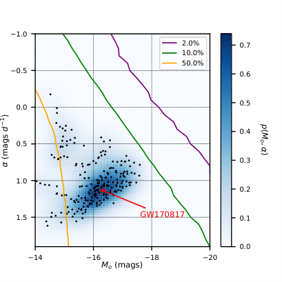
We assume a half opening angle and vary the other three parameters. Using the surrogate models, we predict BNS KN light curves for 10 viewing angles from a polar () to an equatorial () orientation, equally spaced in , and for the following ejecta masses: and in steps of 0.02 . In total, there are 240 BNS KN models. We then map from KN source properties (e.g., ejecta mass and inclination angle) to observables (peak magnitude and evolution rate) by performing lightcurve fits.
A typical simulated BNS KN rapidly rises to a maximum within a day or two and gradually decays. Since the decaying period dominates, we fit a linear model from the entire grid’s median phase of the peak magnitude up to three days since the merger for -, - and -band KN lightcurves. We omitted 20 models that had a mean squared error greater than 0.1 from this process. These omitted models specifically had low but high . For each combination of source parameters, we then combine -, - and -band peak magnitudes and evolution rates based on the number of simulated KNe in simsurvey that fall in the ZTF observed region of any specific filter. For GW190425, we have about 2614, 2930, and 168 out of 100,000 simulated KNe that fall in the region observed with -, - and -band ZTF filters respectively. Gathering the grid-based values for peak absolute magnitudes and decay rates of KNe, we use kernel density estimation to construct a smooth probability density function and approximate the true distribution for the models considered. The left panel of Fig. 5 shows this grid-based prior model overlaid with simsurvey non-detection probabilities.
Effectively, the astrophysical prior reduces a large portion of the parameter space previously considered by the uniform prior choice. The 2%, 10%, and 50% non-detection percentiles estimated using simsurvey are plotted over the astrophysical priors. Though the probable prior region is mostly encompassed by the 50% curve, it lies entirely to the left of the 2% and 10% curves, indicating that our GW190425 ZTF observations are not deep enough to place stringent constraints over the astrophysical priors. This is reflected in the inference results from nimbus (right panel of Fig. 5) based on the astrophysical prior assumptions. Specifically, the posterior and prior contour lines overlap considerably, showing that almost all of the KN models supported by the astrophysical prior survive the upper limits. In general, this implementation demonstrates the ability to use theory and simulation-based astrophysical models within the nimbus framework and constrain them.
| Prior Choice | |
|---|---|
| (mag) | |
| Uniform-mlim | -16.63 |
| Uniform-distance | -15.01 |
| Astrophysical | -17.08 |
IV Discussion and Future Outlook
In this paper, we have presented a hierarchical Bayesian framework nimbus that leverages data from non-detections of probable KNe. This Python package utilizes GW and EM follow-up information from each candidate event to provide posterior distributions for KN model parameters. The framework also accounts for the probability of an event being astrophysical. Although the analysis presented here focuses on a single BNS event, GW190425, the framework has the capability to include multiple events. It is also straightforward to extend the framework to model the inference based on sub-populations of KN candidates such as BNS and NSBH mergers. We hope the multi-messenger astrophysics community finds use for and benefits from this package.
A current limitation of this study is that the framework does not account for events that have been detected in EM follow-up. In order to place stringent constraints on KN parameters, it would be ideal to include potential candidates for which there exists data from detected light curves. However, including information from detected events into the framework would involve non-trivial changes to the model likelihood and would necessitate an accurate understanding of survey selection effects. So far, GW170817 (Abbott et al. 2017b) is the only GW event to have been associated with a KN counterpart (Abbott et al. 2017). Numerous studies in the literature (Cowperthwaite et al. 2017; Drout et al. 2017; Arcavi 2018; Andreoni et al. 2020, e.g.,) have extrapolated follow-up data to arrive at an estimate of its initial absolute magnitude and decay rate. In particular, Kasliwal et al. 2020 compared their results to an extrapolated initial magnitude of mag with a decay rate of mag per day. Our results do indicate non-negligible posterior support for such a model. Nevertheless, this represents a single point in model parameter space and we would instead require a number of detected events to inform the population of KNe. Further, restricting the study to non-detections is motivated by the fact that O3 did not yield any obvious EM counterparts. We defer the development of including detected events to a future study.
We presented results of our inference on GW190425 using two different prior choices for our model parameters (see Figs. 1 and 5). Our first choice, which is uniform in the parameters, is representative of an inference that is carried out with uninformative assumptions. Our second prior choice is based on surrogate models from Monte-Carlo radiative transfer simulations of KNe (Coughlin et al. 2018a; Bulla 2019) and takes into account the effect of variations in ejecta masses and inclination angle on the resulting KN morphology. The inference using such a prior represents the possibility of testing realistic, physical models of KNe against upper limits obtained from surveys. While our implementation with uniform priors constrained the prior parameter space to a considerable extent and shows consistency with previous efforts (Kasliwal et al. 2020), the posterior results based on surrogate KNe models are largely uninformative with respect to the prior. Overall, these results show how priors on model parameters can influence the constraints obtained and the need to examine results in light of the prior distribution.
One of the assumptions we have made in presenting our results above is that the KN counterpart to GW190425 is localized within the surveyed region of the skymap. GW190425, as mentioned previously in Sec. III, had an overall sky coverage by ZTF of . Given that a significant fraction of the skymap is not surveyed and therefore would result in uninformative constraints, we made this assumption to demonstrate the utility of the Bayesian framework. In LIGO-Virgo-KAGRA’s fourth observing run, we expect that for 8-10% of BNS and NSBH systems discovered, ZTF will be able to observe 90% of the localization (Petrov et al. 2021), and hence our above assumption would hold reasonably true in those particular cases.
Furthermore, throughout this study we have assumed a kilonova luminosity evolution model that is linear in time. A linear model only needs two parameters to define it and our goal in this paper has been to demonstrate framework functionality at the cost of model accuracy. Such a simplistic choice might not be representative of realistic evolution models (see Metzger 2019) that depend on more complex parameters related to the binary system. In principle, it should be feasible to include arbitrary models for luminosity evolution since the framework only expects a function that returns predictions for the absolute magnitude of the KN as a function of time. For all priors applied, we consider only the first three days of evolution of the KN (and therefore the first three days of observations after the merger time of GW190425). This choice is motivated by the fact that ZTF is unlikely to detect a KN at the distance of GW190425 in the - and -bands after three days post-merger. More specifically, at four days, all KN models in our set have an apparent magnitude in the - and -bands fainter than the median depth of ZTF in this study ( 21 mag).
In this work we also neglected color evolution in our studies of kilonova non-detections. In addition to differentiating observations in different filters, in the future we intend to account for the K-correction effect on kilonova color evolution which is especially relevant for cosmological sources. We will implement this feature in nimbus following the existing implementation in simsurvey.
We highlight here that due to the adaptability of nimbus to various lightcurve models and a hierarchical framework, it could even be used to jointly constrain the properties of a potential kilonova and short GRB optical afterglow associated with the GW event (as in Dietrich et al. 2020, Pang et al. in prep) based on the rapid optical follow-up performed by various facilities.
In order to establish consistency with existing results in the literature, we compared our results to those from the simulator software simsurvey. As shown in Fig. 4, the two formalisms are largely consistent although some qualitative differences exist. In the future, with observations and upper limits from more events, it will be possible to test for further consistency between frameworks investigating KN populations.
In our specific implementation with astrophysical priors in Sec. III.1, we used a prior on the KN luminosity parameters, i.e. the initial absolute magnitude and evolution rate that depends on intrinsic parameters such as the dynamical or wind ejecta masses. Our Bayesian approach makes it straightforward to convert our posteriors on the luminosity parameters into constraints on these intrinsic parameters. Alternatively, since the framework is agnostic to the KN model used, it should be possible to directly use priors on the physical parameters that govern the light-curve morphology. In such a case, the inference would directly constrain parameters such as the ejecta mass from the binary merger, although the computational feasibility of such an implementation needs to be investigated. The use of these astrophysical priors is based on including variations in the observer viewing (inclination) angle and its effect on each KN model. Non-trivial couplings between the observer angle and the signal-to-noise ratio of the GW signal can lead to some selection bias. To mitigate this effect in the future, we will select skymaps from a realistic distribution of GW signals detected by LIGO (Petrov et al. 2021) which will inform the distribution of observer angles for our kilonova models.
Looking forward to O4 and beyond, we expect that nimbus will be an important framework for analyzing joint EM-GW observations. Petrov et al. 2021 predict a median of 35 BNS yr-1 with O4 sensitivity and roughly double the number during O5. Thus, with several tens of EM follow-ups of BNS events from O4 and O5, we will use nimbus to place stringent population-level luminosity function constraints based on non-detections. For the well-localized ( deg2) and nearby ( Mpc) events (predicted to range from 0-13 BNS mergers; Petrov et al. 2021) detected by LIGO in O4 for which we have excellent optical sky coverage, nimbus is ideally placed to constrain the intrinsic kilonova properties which can translate to constraints on binary system parameters such as mass ratio and NS radius in the face of non-detection. A similar analysis of NSBH mergers is also feasible, though ejecta mass yield sensitively depends on the mass ratio of the system (e.g. Krüger & Foucart 2020). As a follow-up study, we hope to explore the scientific merit of conducting EM-GW follow-ups with the Vera C. Rubin Observatory, assuming the cadence and filter strategy for KN identification outlined in (Andreoni et al. 2021), using the nimbus framework.
Constraining the ejecta masses of the KN population could potentially provide us better insights into the amount of -process material contributed to the formation of KNe (Hotokezaka et al. 2018). It will also help in understanding the relationship and breaking the degeneracy that exists between binary parameters (equation of state, spin and mass ratio) (Foucart et al. 2018; Hinderer et al. 2019; Radice & Dai 2019; Zhu et al. 2020), ejecta mass and KN light curve morphology. (Coughlin et al. 2019a; Hotokezaka & Nakar 2020; Breschi et al. 2021; Raaijmakers et al. 2021). The future GW and EM multi-messenger landscape will provide the opportunity to explore this further.
References
- Aasi et al. (2015) Aasi, J., Abbott, B. P., Abbott, R., et al. 2015, Classical and Quantum Gravity, 32, 074001
- Abbott et al. (2017a) Abbott, B. P., Abbott, R., Abbott, T. D., et al. 2017a, The Astrophysical Journal, 850, L39
- Abbott et al. (2017b) —. 2017b, Phys. Rev. Lett., 119, 161101
- Abbott et al. (2017) Abbott, B. P., Abbott, R., Abbott, T. D., et al. 2017, ApJ, 848, L12
- Abbott et al. (2019) —. 2019, Physical Review X, 9, 031040
- Abbott et al. (2020) Abbott, B. P., et al. 2020, arXiv:2001.01761
- Abbott et al. (2020) Abbott, R., Abbott, T. D., Abraham, S., et al. 2020, arXiv e-prints, arXiv:2010.14527
- Acernese et al. (2015) Acernese, F., et al. 2015, Class. Quant. Grav., 32, 024001
- Anand et al. (2020) Anand, S., Coughlin, M. W., Kasliwal, M. M., et al. 2020, Nature Astronomy, doi:10.1038/s41550-020-1183-3
- Andreoni et al. (2020) Andreoni, I., Goldstein, D., et al. 2020, Astrophys. J., 890, 131
- Andreoni et al. (2017) Andreoni, I., Ackley, K., Cooke, J., et al. 2017, PASA, 34, e069
- Andreoni et al. (2021) Andreoni, I., Coughlin, M. W., Kool, E. C., et al. 2021, Fast-transient Searches in Real Time with ZTFReST: Identification of Three Optically-discovered Gamma-ray Burst Afterglows and New Constraints on the Kilonova Rate, , , arXiv:2104.06352
- Andreoni et al. (2021) Andreoni, I., Margutti, R., Sharan Salafia, O., et al. 2021, arXiv e-prints, arXiv:2111.01945
- Antier et al. (2020) Antier, S., Agayeva, S., AlMualla, M., et al. 2020, arXiv:2004.04277
- Arcavi (2018) Arcavi, I. 2018, The Astrophysical Journal, 855, L23
- Barbieri et al. (2020) Barbieri, C., Salafia, O. S., Colpi, M., Ghirlanda, G., & Perego, A. 2020, arXiv:2002.09395
- Barnes et al. (2016) Barnes, J., Kasen, D., Wu, M.-R., & Martínez-Pinedo, G. 2016, ApJ, 829, 110
- Barnes et al. (2020) Barnes, J., Zhu, Y. L., Lund, K. A., et al. 2020, arXiv e-prints, arXiv:2010.11182
- Bauswein et al. (2013) Bauswein, A., Baumgarte, T. W., & Janka, H.-T. 2013, Phys. Rev. Lett., 111, 131101
- Bellm et al. (2019) Bellm, E. C., Kulkarni, S. R., Graham, M. J., et al. 2019, Publications of the Astronomical Society of the Pacific, 131, 018002
- Blazek et al. (2019) Blazek, M., Christensen, N., Howell, E., et al. 2019, GRB Coordinates Network, 24227, 1
- Breschi et al. (2021) Breschi, M., Perego, A., Bernuzzi, S., et al. 2021, arXiv e-prints, arXiv:2101.01201
- Bulla (2019) Bulla, M. 2019, Monthly Notices of the Royal Astronomical Society, 489, 5037–5045
- Chambers et al. (2016) Chambers, K. C., Magnier, E. A., Metcalfe, N., et al. 2016, arXiv e-prints, arXiv:1612.05560
- Chornock et al. (2017) Chornock, R., Berger, E., Kasen, D., et al. 2017, The Astrophysical Journal, 848, L19
- Côté et al. (2018) Côté, B., Fryer, C. L., Belczynski, K., et al. 2018, ApJ, 855, 99
- Coughlin et al. (2019a) Coughlin, M. W., Dietrich, T., Margalit, B., & Metzger, B. D. 2019a, Monthly Notices of the Royal Astronomical Society: Letters, 489, L91
- Coughlin et al. (2018a) Coughlin, M. W., Dietrich, T., Doctor, Z., et al. 2018a, Monthly Notices of the Royal Astronomical Society, 480, 3871–3878
- Coughlin et al. (2018b) Coughlin, M. W., Tao, D., Chan, M. L., et al. 2018b, Monthly Notices of the Royal Astronomical Society, 478, 692–702
- Coughlin et al. (2019b) Coughlin, M. W., Ahumada, T., Cenko, S. B., et al. 2019b, Publications of the Astronomical Society of the Pacific, 131, 048001
- Coughlin et al. (2019c) Coughlin, M. W., Ahumada, T., Anand, S., et al. 2019c, The Astrophysical Journal, 885, L19
- Coughlin et al. (2019d) Coughlin, M. W., Dietrich, T., Antier, S., et al. 2019d, Mon. Not. Roy. Astron. Soc., 492, 863
- Coulter et al. (2017) Coulter, D. A., Foley, R. J., Kilpatrick, C. D., et al. 2017, Science, 358, 1556
- Cowperthwaite et al. (2017) Cowperthwaite, P. S., Berger, E., Villar, V. A., et al. 2017, ApJ, 848, L17
- De et al. (2019) De, K., Adams, S. M., Coughlin, M., et al. 2019, GRB Coordinates Network, 24187, 1
- Dekany et al. (2020) Dekany, R., Smith, R. M., Riddle, R., et al. 2020, PASP, 132, 038001
- Dhawan et al. (2020) Dhawan, S., Bulla, M., Goobar, A., Sagués Carracedo, A., & Setzer, C. N. 2020, ApJ, 888, 67
- Dietrich et al. (2020) Dietrich, T., Coughlin, M. W., Pang, P. T. H., et al. 2020, Science, 370, 1450
- Drout et al. (2017) Drout, M. R., Piro, A. L., Shappee, B. J., et al. 2017, Science, 358, 1570
- Dudi et al. (2021) Dudi, R., Adhikari, A., Brügmann, B., et al. 2021, arXiv e-prints, arXiv:2109.04063
- Etienne et al. (2009) Etienne, Z. B., Liu, Y. T., Shapiro, S. L., & Baumgarte, T. W. 2009, Phys. Rev. D, 79, 044024
- Evans et al. (2017) Evans, P. A., Cenko, S. B., Kennea, J. A., et al. 2017, Science, 358, 1565
- Farr et al. (2015) Farr, W. M., Gair, J. R., Mandel, I., & Cutler, C. 2015, Phys. Rev. D, 91, 023005
- Feindt et al. (2019) Feindt, U., Nordin, J., Rigault, M., et al. 2019, Journal of Cosmology and Astroparticle Physics, 2019, 005–005
- Foley et al. (2020) Foley, R. J., Coulter, D. A., Kilpatrick, C. D., et al. 2020, Monthly Notices of the Royal Astronomical Society, 494, 190
- Foucart et al. (2018) Foucart, F., Hinderer, T., & Nissanke, S. 2018, Phys. Rev. D, 98, 081501
- Foucart et al. (2021) Foucart, F., Moesta, P., Ramirez, T., et al. 2021, arXiv e-prints, arXiv:2109.00565
- Gaebel et al. (2019) Gaebel, S. M., Veitch, J., Dent, T., & Farr, W. M. 2019, Monthly Notices of the Royal Astronomical Society, 484, 4008
- Ghosh et al. (2017) Ghosh, S., Chatterjee, D., Kaplan, D. L., Brady, P. R., & Sistine, A. V. 2017, Publications of the Astronomical Society of the Pacific, 129, 114503
- Gompertz et al. (2020) Gompertz, B., et al. 2020, arXiv:2004.00025
- Górski et al. (2005) Górski, K. M., Hivon, E., Banday, A. J., et al. 2005, ApJ, 622, 759
- Graham et al. (2019) Graham, M. J., Kulkarni, S. R., Bellm, E. C., et al. 2019, Publications of the Astronomical Society of the Pacific, 131, 078001
- Green (2018) Green, G. 2018, The Journal of Open Source Software, 3, 695
- Harris et al. (2020) Harris, C. R., Millman, K. J., van der Walt, S. J., et al. 2020, Nature, 585, 357–362
- Heinzel et al. (2021) Heinzel, J., Coughlin, M. W., Dietrich, T., et al. 2021, MNRAS, arXiv:2010.10746
- Hinderer et al. (2019) Hinderer, T., Nissanke, S., Foucart, F., et al. 2019, Phys. Rev. D, 100, 063021
- Hosseinzadeh et al. (2019) Hosseinzadeh, G., Cowperthwaite, P. S., Gomez, S., et al. 2019, ApJ, 880, L4
- Hotokezaka et al. (2018) Hotokezaka, K., Beniamini, P., & Piran, T. 2018, International Journal of Modern Physics D, 27, 1842005
- Hotokezaka et al. (2013) Hotokezaka, K., Kiuchi, K., Kyutoku, K., et al. 2013, Phys. Rev. D, 87, 024001
- Hotokezaka & Nakar (2020) Hotokezaka, K., & Nakar, E. 2020, ApJ, 891, 152
- Hotokezaka et al. (2019) Hotokezaka, K., Nakar, E., Gottlieb, O., et al. 2019, Nature Astronomy, 3, 940
- Hunter (2007) Hunter, J. D. 2007, Computing in Science Engineering, 9, 90
- Just et al. (2021) Just, O., Kullmann, I., Goriely, S., et al. 2021, arXiv e-prints, arXiv:2109.14617
- Kasen et al. (2015) Kasen, D., Fernández, R., & Metzger, B. D. 2015, MNRAS, 450, 1777
- Kasen et al. (2017) Kasen, D., Metzger, B., Barnes, J., Quataert, E., & Ramirez-Ruiz, E. 2017, Nature, 551, 80
- Kasliwal (2011) Kasliwal, M. M. 2011, PhD thesis, California Institute of Technology
- Kasliwal et al. (2017) Kasliwal, M. M., Nakar, E., Singer, L. P., et al. 2017, Science, 358, 1559
- Kasliwal et al. (2019a) Kasliwal, M. M., Coughlin, M. W., Bellm, E. C., et al. 2019a, GRB Coordinates Network, 24191, 1
- Kasliwal et al. (2019b) Kasliwal, M. M., Kasen, D., Lau, R. M., et al. 2019b, MNRAS, arXiv:1812.08708
- Kasliwal et al. (2020) Kasliwal, M. M., Anand, S., Ahumada, T., et al. 2020, Kilonova Luminosity Function Constraints based on Zwicky Transient Facility Searches for 13 Neutron Star Mergers, , , arXiv:2006.11306
- Kawaguchi et al. (2016) Kawaguchi, K., Kyutoku, K., Shibata, M., & Tanaka, M. 2016, The Astrophysical Journal, 825, 52
- Kawaguchi et al. (2020) Kawaguchi, K., Shibata, M., & Tanaka, M. 2020, ApJ, 889, 171
- Kilpatrick et al. (2017) Kilpatrick, C. D., Foley, R. J., Kasen, D., et al. 2017, Science, 358, 1583
- Kiuchi et al. (2019) Kiuchi, K., Kyutoku, K., Shibata, M., & Taniguchi, K. 2019, The Astrophysical Journal, 876, L31
- Kluyver et al. (2016) Kluyver, T., Ragan-Kelley, B., Pérez, F., et al. 2016, in Positioning and Power in Academic Publishing: Players, Agents and Agendas, ed. F. Loizides & B. Scmidt (Netherlands: IOS Press), 87–90
- Korobkin et al. (2020) Korobkin, O., Wollaeger, R., Fryer, C., et al. 2020, arXiv e-prints, arXiv:2004.00102
- Krüger & Foucart (2020) Krüger, C. J., & Foucart, F. 2020, Phys. Rev. D, 101, 103002
- Kullmann et al. (2021) Kullmann, I., Goriely, S., Just, O., et al. 2021, arXiv e-prints, arXiv:2109.02509
- Kyutoku et al. (2020) Kyutoku, K., Fujibayashi, S., Hayashi, K., et al. 2020, ApJ, 890, L4
- Kyutoku et al. (2015) Kyutoku, K., Ioka, K., Okawa, H., Shibata, M., & Taniguchi, K. 2015, Phys. Rev. D, 92, 044028
- Köppel et al. (2019) Köppel, S., Bovard, L., & Rezzolla, L. 2019, The Astrophysical Journal, 872, L16
- Levan (2020) Levan, A. 2020, PoS, Asterics2019, 044
- Li et al. (2019) Li, B., Xu, D., Zhou, X., & Lu, H. 2019, GRB Coordinates Network, 24285, 1
- Li & Paczyński (1998) Li, L.-X., & Paczyński, B. 1998, The Astrophysical Journal, 507, L59–L62
- Lipunov et al. (2019) Lipunov, V., Gorbovskoy, E., Kornilov, V., et al. 2019, GRB Coordinates Network, 24167, 1
- Lipunov et al. (2017) Lipunov, V. M., Gorbovskoy, E., Kornilov, V. G., et al. 2017, ApJ, 850, L1
- Lundquist et al. (2019a) Lundquist, M. J., Paterson, K., Sand, D. J., et al. 2019a, GRB Coordinates Network, 24172, 1
- Lundquist et al. (2019b) Lundquist, M. J., Paterson, K., Fong, W., et al. 2019b, ApJ, 881, L26
- Mandel et al. (2019) Mandel, I., Farr, W. M., & Gair, J. R. 2019, Monthly Notices of the Royal Astronomical Society, 486, 1086
- Masci et al. (2019) Masci, F. J., Laher, R. R., Rusholme, B., et al. 2019, Publications of the Astronomical Society of the Pacific, 131, 018003
- McBrien et al. (2019) McBrien, O., Smartt, S., Smith, K. W., et al. 2019, GRB Coordinates Network, 24197, 1
- McCully et al. (2017) McCully, C., Hiramatsu, D., Howell, D. A., et al. 2017, ApJ, 848, L32
- Metzger (2019) Metzger, B. D. 2019, Living Reviews in Relativity, 23, arXiv:1910.01617
- Metzger et al. (2010) Metzger, B. D., Martínez-Pinedo, G., Darbha, S., et al. 2010, Monthly Notices of the Royal Astronomical Society, 406, 2650
- Mohite (2021) Mohite, S. R. 2021, nimbus : A Bayesian inference framework to constrain kilonova models., v.v1.0.0, Zenodo, doi:10.5281/zenodo.5648468
- Morgan et al. (2020) Morgan, R., Soares-Santos, M., Annis, J., et al. 2020, ApJ, 901, 83
- Nakar (2019) Nakar, E. 2019, arXiv:1912.05659
- Nicholl et al. (2021) Nicholl, M., Margalit, B., Schmidt, P., et al. 2021, Monthly Notices of the Royal Astronomical Society, 505, 3016
- Nicholl et al. (2017) Nicholl, M., Berger, E., Kasen, D., et al. 2017, ApJ, 848, L18
- Pedregosa et al. (2011) Pedregosa, F., Varoquaux, G., Gramfort, A., et al. 2011, Journal of Machine Learning Research, 12, 2825
- Perego et al. (2017) Perego, A., Radice, D., & Bernuzzi, S. 2017, ApJ, 850, L37
- Pérez & Granger (2007) Pérez, F., & Granger, B. E. 2007, Computing in Science and Engineering, 9, 21
- Petrov et al. (2021) Petrov, P., Singer, L. P., Coughlin, M. W., et al. 2021, arXiv e-prints, arXiv:2108.07277
- Pian et al. (2017) Pian, E., D’Avanzo, P., Benetti, S., et al. 2017, Nature, 551, 67
- Raaijmakers et al. (2021) Raaijmakers, G., Nissanke, S., Foucart, F., et al. 2021, arXiv:2102.11569
- Radice & Dai (2019) Radice, D., & Dai, L. 2019, European Physical Journal A, 55, 50
- Radice et al. (2018) Radice, D., Perego, A., Hotokezaka, K., et al. 2018, ApJ, 869, 130
- Roberts et al. (2011) Roberts, L. F., Kasen, D., Lee, W. H., & Ramirez-Ruiz, E. 2011, ApJ, 736, L21
- Rosswog (2005) Rosswog, S. 2005, The Astrophysical Journal, 634, 1202
- Rosswog et al. (2017) Rosswog, S., Feindt, U., Korobkin, O., et al. 2017, Classical and Quantum Gravity, 34, 104001
- Sagués Carracedo et al. (2021) Sagués Carracedo, A., Bulla, M., Feindt, U., & Goobar, A. 2021, MNRAS, 504, 1294
- Sasada et al. (2021) Sasada, M., Utsumi, Y., Itoh, R., et al. 2021, Progress of Theoretical and Experimental Physics, 2021, 05A104
- Schlafly & Finkbeiner (2011) Schlafly, E. F., & Finkbeiner, D. P. 2011, The Astrophysical Journal, 737, 103
- Shappee et al. (2017) Shappee, B. J., Simon, J. D., Drout, M. R., et al. 2017, Science, 358, 1574
- Siegel (2019) Siegel, D. M. 2019, European Physical Journal A, 55, 203
- Singer & Price (2016) Singer, L. P., & Price, L. R. 2016, Phys. Rev. D, 93, 024013
- Singer et al. (2016a) Singer, L. P., Chen, H.-Y., Holz, D. E., et al. 2016a, The Astrophysical Journal, 829, L15
- Singer et al. (2016b) —. 2016b, The Astrophysical Journal Supplement Series, 226, 10
- Smartt et al. (2017) Smartt, S. J., Chen, T. W., Jerkstrand, A., et al. 2017, Nature, 551, 75
- Smith et al. (2019) Smith, K., Young, D., McBrien, O., et al. 2019, GRB Coordinates Network, 24210, 1
- Soares-Santos et al. (2017) Soares-Santos, M., Holz, D., Annis, J., Chornock, R., & Herner, K. 2017, Astrophys. J. Lett., 848, L16
- Steeghs et al. (2019) Steeghs, D., Dyer, M., Galloway, D., et al. 2019, GRB Coordinates Network, 24224, 1
- Tanaka (2016) Tanaka, M. 2016, Advances in Astronomy, 2016, 634197
- Tanaka & Hotokezaka (2013) Tanaka, M., & Hotokezaka, K. 2013, The Astrophysical Journal, 775, 113
- Tanaka et al. (2017) Tanaka, M., Utsumi, Y., Mazzali, P. A., et al. 2017, PASJ, 69, 102
- Tanaka et al. (2018) Tanaka, M., Kato, D., Gaigalas, G., et al. 2018, The Astrophysical Journal, 852, 109
- Tanvir et al. (2017) Tanvir, N. R., Levan, A. J., González-Fernández, C., et al. 2017, ApJ, 848, L27
- Tonry et al. (2018) Tonry, J. L., Denneau, L., Heinze, A. N., et al. 2018, Publications of the Astronomical Society of the Pacific, 130, 064505
- Utsumi et al. (2017) Utsumi, Y., Tanaka, M., Tominaga, N., et al. 2017, PASJ, 69, 101
- Van Rossum & Drake (2009) Van Rossum, G., & Drake, F. L. 2009, Python 3 Reference Manual (Scotts Valley, CA: CreateSpace)
- Veitch et al. (2015) Veitch, J., Raymond, V., Farr, B., et al. 2015, Phys. Rev. D, 91, 042003
- Virtanen et al. (2020) Virtanen, P., Gommers, R., Oliphant, T. E., et al. 2020, Nature Methods, 17, 261
- Waxman et al. (2018) Waxman, E., Ofek, E. O., Kushnir, D., & Gal-Yam, A. 2018, MNRAS, 481, 3423
- Wollaeger et al. (2018) Wollaeger, R. T., Korobkin, O., Fontes, C. J., et al. 2018, MNRAS, 478, 3298
- Wu et al. (2019) Wu, M.-R., Barnes, J., Martínez-Pinedo, G., & Metzger, B. D. 2019, Phys. Rev. Lett., 122, 062701
- Xu et al. (2019) Xu, D., Zhu, Z. P., Yu, B. Y., et al. 2019, GRB Coordinates Network, 24190, 1
- Zhu et al. (2021) Zhu, J.-P., Yang, Y.-P., Zhang, B., Gao, H., & Yu, Y.-W. 2021, arXiv e-prints, arXiv:2110.10468
- Zhu et al. (2020) Zhu, J.-P., Wu, S., Yang, Y.-P., et al. 2020, arXiv e-prints, arXiv:2011.02717
- Zhu et al. (2018) Zhu, Y., Wollaeger, R. T., Vassh, N., et al. 2018, The Astrophysical Journal, 863, L23