Uncertainty-Aware Reliable Text ClassificationConference: Proceedings of the 27th ACM SIGKDD Conference on Knowledge Discovery and Data Mining; August 14–18, 2021; Virtual Event, SingaporeProceedings of the 27th ACM SIGKDD Conference on Knowledge Discovery and Data Mining (KDD ’21), August 14–18, 2021, Virtual Event, SingaporeDOI: 10.1145/3447548.3467382ISBN: 978-1-4503-8332-5/21/08rst2800CCS: Computing methodologies Natural language processingCCS: Computing methodologies Neural networks
Abstract.
Deep neural networks have significantly contributed to the success in predictive accuracy for classification tasks. However, they tend to make over-confident predictions in real-world settings, where domain shifting and out-of-distribution (OOD) examples exist. Most research on uncertainty estimation focuses on computer vision because it provides visual validation on uncertainty quality. However, few have been presented in the natural language process domain. Unlike Bayesian methods that indirectly infer uncertainty through weight uncertainties, current evidential uncertainty-based methods explicitly model the uncertainty of class probabilities through subjective opinions. They further consider inherent uncertainty in data with different root causes, vacuity (i.e., uncertainty due to a lack of evidence) and dissonance (i.e., uncertainty due to conflicting evidence). In our paper, we firstly apply evidential uncertainty in OOD detection for text classification tasks. We propose an inexpensive framework that adopts both auxiliary outliers and pseudo off-manifold samples to train the model with prior knowledge of a certain class, which has high vacuity for OOD samples. Extensive empirical experiments demonstrate that our model based on evidential uncertainty outperforms other counterparts for detecting OOD examples. Our approach can be easily deployed to traditional recurrent neural networks and fine-tuned pre-trained transformers.
Keywords:
out-of-distribution detection; uncertainty qualification; text classification1. Introduction
Deep neural networks have significantly contributed to the success of predictive accuracy for classification tasks in multiple domains. However, many applications require confidence in reliability. In real-world settings that contain out-of-distribution (OOD) samples, the model should know when it can not make a confident judgment rather than making an incorrect one. Studies show that traditional neural networks easily lead to over-confidence, i.e., a high-class probability in an incorrect class prediction (Guo et al. 2017; Hein et al. 2019; Ovadia et al. 2019). Therefore, calibrated predictive uncertainty is crucial to avoid those risks.
In this paper, we are interested in qualifying uncertainty to solve OOD detection in text classification as it contains a wide range of Natural Language Processing (NLP) applications (Chang et al. 2020; Li and Ye 2018). Although fine-tuning pre-trained transformers (Devlin et al. 2018) have achieved state-of-the-art accuracy on text classification tasks, they still suffer from the same over-confidence problem of traditional neural networks, making the prediction untrustful (Hendrycks et al. 2020). One partial explanation is over-parameterization (Guo et al. 2017). Although transformers are pre-trained on a large corpus and get rich semantic information, it leads to over-confidence easily given limited labeled data during the fine-tuning stage (Kong et al. 2020). Overall, compared to the Computer Vision (CV) domain, there is less work in qualifying uncertainty in the NLP domain. Among them, there are Bayesian and non-Bayesian methods.
Bayesian models qualify the model uncertainty by Bayesian neural networks (BNNs) (Blundell et al. 2015; Louizos and Welling 2017). BNNs explicitly qualify model uncertainty by considering model parameters as distributions. Specifically, BNNs consider probabilistic uncertainty, i.e., aleatoric uncertainty and epistemic uncertainty (Kendall and Gal 2017). Aleatoric only considers data uncertainty caused by statistical randomness. At the same time, epistemic refers to model uncertainty introduced by limited knowledge or ignorance in collected data. Monte Carlo Dropout (Gal and Ghahramani 2016) is a crucial technique to approximate variational Bayesian inference. It trains and evaluates a neural network with dropout (Srivastava et al. 2014) before each layer. BNNs have been explored for classification prediction or regression in CV applications. However, there has been less study in the NLP domain. Few work (Xiao and Wang 2019; Van Landeghem et al. 2020; Ovadia et al. 2019) empirically evaluate uncertainty estimation in text classification. Other attempts adopt MC Dropout in deep active learning (Shen et al. 2017; Siddhant and Lipton 2018), sentiment analysis (Andersen et al. 2020), or machine translation (Zhou et al. 2020).
Non-Bayesian approaches use entropy (Shannon 1948) or softmax scores as a measure of uncertainty, which only considers aleatoric uncertainty (Kendall and Gal 2017). OOD detection in text classification using GRU (Chung et al. 2014) or LSTM (Hochreiter and Schmidhuber 1997) has been studied in (Hendrycks and Gimpel 2016; Hendrycks et al. 2018). Hendrycks et al. 2020 empirically study pre-trained transformers’ performance on OOD detection. They point out transformers cannot clearly separate in-distribution (ID) and OOD examples. In addition, OOD detection has also been studied in dialogue systems (Zheng et al. 2020) and document classification (Zhang et al. 2019; He et al. 2020). Another line of non-Bayesian methods involves the calibration of probabilities. Temperature scaling (Guo et al. 2017) calibrates softmax probabilities by adding a scalar parameter to each class in a post-processing step. Thulasidasan et al. 2019 explore the improvement of calibration and predictive uncertainty of models trained with mix-up (Zhang et al. 2017) in the NLP domain. Kong et al. 2020 use pseudo samples on and off the data manifold for calibration.
| Calibrated? | Test Sentence | Probability | Dirichlet | Uncertainty | |
|---|---|---|---|---|---|
| No | 3. ’Deep learning is data hungry.’ | = [0.99, 0.1] | doesn’t apply | Over-confidence | |
| Yes |
|
= [0.01, 0.99] | = [1,99] | Low uncertainty | |
|
= [0.5, 0.5] | = [50, 50] |
| ||
| 3. ’Deep learning is data hungry.’ | = [0.5, 0.5] | = [1, 1] |
|
Besides probabilistic uncertainty and BNNs, evidential uncertainty is proposed based on belief/evidence theory and Subjective Logic (SL) (Jøsang 2016; Jøsang et al. 2018). It considers different dimensions of uncertainty, such as vacuity (i.e., lack of evidence) or dissonance (i.e., uncertainty due to conflicting evidence). In the CV domain, Sensoy et al. 2020 propose evidential neural networks (ENNs) to model the uncertainty of class probabilities based on SL explicitly. An ENN uses the predictions as subjective opinions and learns a function that collects evidence to form the opinions by a deterministic neural network from data. Several works (Sensoy et al. 2020; Zhao et al. 2019; Hu et al. 2020) improve ENNs using regularization or generative models to ensure correct uncertainty estimation towards unseen examples in image classification. However, those methods for continuous feature space are not applicable to the discrete text.
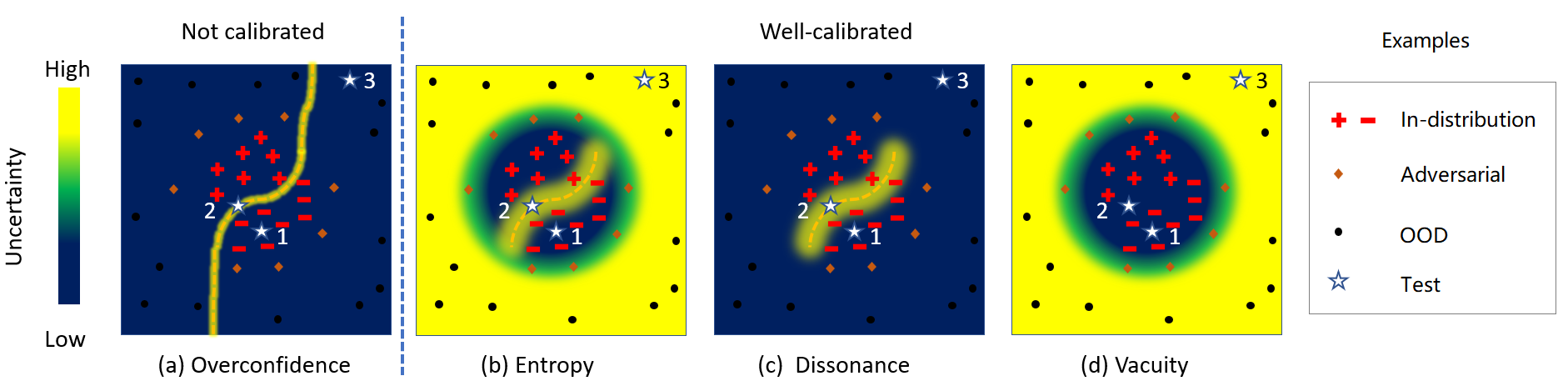
To briefly demonstrate the motivation of our paper, we use a simple binary classification example in Table 1 and Figure 1 to answer the following questions:
- •
Why is it necessary to calibrate predictive uncertainty?
- •
What is the advantage of evidential uncertainty in OOD detection?
- •
How to design a regularization method to calibrate the predictive uncertainty?
In Table 1, we assume that a classifier is only trained on the restaurant reviews dataset and has never seen examples from other domains. The probability denotes the prediction softmax probability. The evidence represents historical observations, denoted by Dirichlet distributions (no evidence when ). Before calibration, the classifier predicts Sentence 3, an obvious OOD example, as positive with high confidence. Thus it is necessary to calibrate predictive uncertainty is to reduce over-confidence.
For a well-calibrated model, there are three common cases in predictions. Sentence 1 refers to correct confident classification, where we have enough evidence with no conflicts. Sentence 2 is vague and contains conflicting information like ’bad’ and ’acceptable’. The prediction will result in equal probability because each category supports equal evidence, i.e., conflicting evidence or high dissonance. Finally, we lack the evidence to support our prediction for an OOD sample, Sentence 3. It results in high vacuity with Dirichlet distribution being a uniform distribution. The model outputs the same predictive probability for Sentence 2 and 3, which have pretty different evidence. In this case, probabilistic uncertainty cannot distinguish the conflicting case and the out-of-distribution case. Evidential uncertainty decomposes the uncertainty base on different root causes. This explains the advantage of evidential uncertainty over probabilistic uncertainty.
Figure 1 illustrates the prediction uncertainty of neural networks in Table 1. Assume we project the examples in a 2D space. Sentence 1 lies in the region with many negative examples. Sentence 2 lies in the boundary region. Sentence 3 is far away from the ID region. Figure 1 (a) represents the prediction by traditional neural networks with softmax and demonstrates over-confidence. It only assigns high uncertainty (entropy) near the classification boundary. Hein et al. 2019 prove that ReLU type neural networks produce arbitrary high confidence predictions far away from the training data. Figure 1 (b) represents the predictive entropy of a well-calibrated model. Figure 1 (c) and (d) shows the evidential uncertainty decomposes the uncertainty in (b) based on different root causes. We observe high vacuity in OOD regions and high dissonance in ID boundary regions. Vacuity can effectively detect OOD samples from boundary ID examples because the cause of uncertainty is due to a lack of evidence. We can distinguish sentence 3 from sentence 2 in Figure 1 (c) but not in Figure 1 (b).
Finally, in Figure 1 we also observe OOD examples and adversarial examples. Adversarial examples (Szegedy et al. 2013; Carlini and Wagner 2017; Madry et al. 2017) refer to instances with small feature perturbations. A lot of studies (Jia and Liang 2017; Wallace et al. 2019; Jia et al. 2019) use adversarial examples to evaluate and improve neural networks’ robustness. We can use diverse outliers to calibrate the model to output high uncertainty in the OOD region (Hendrycks et al. 2018). Additionally, adversarial examples can be helpful to detect OOD examples close to ID regions. Thus, our approach adopts a mixture of an auxiliary dataset of outliers and close adversarial examples to calibrate the predictive uncertainty. We can easily get diverse text data as auxiliary outliers. However, generating adversarial examples via common gradient-based approaches is impossible in the NLP domain. Thus, we apply methods (Stutz et al. 2019; Gilmer et al. 2018; Kong et al. 2020) to generate off-manifold adversarial examples from the embedding layer.
Our work provides the following key contributions : (i) We firstly apply evidential uncertainty to solve OOD detection tasks in the text classification. (ii) We propose an inexpensive framework that adopts both an auxiliary dataset of outliers and generated pseudo off-manifold samples to train a model with prior knowledge of a certain class, which has high vacuity for OOD samples. (iii) We validate our proposed method’s performance via extensive experiments of OOD detection and uncertainty estimation in text classification. Our approach significantly outperforms all the counterparts.
2. Preliminaries
We briefly provide the background knowledge of evidential uncertainty and the advantage over probabilistic uncertainty.
2.1. Subjective Opinions in SL
A multinomial opinion in a given proposition is represented by where a domain is , a random variable takes value in , and is given as . denotes belief mass function over . denotes uncertainty mass representing vacuity of evidence. represents base rate distribution over , with . Then the projected probability distribution of a multinomial opinion is given by:
| (1) |
Multinomial probability density over a domain of cardinality is represented by the -dimensional Dirichlet PDF where the special case with is the Beta PDF as a binomial opinion. It denotes a domain of mutually disjoint elements in and the strength vector over and the probability distribution over .
| (2) |
where is a multivariate beta function as the normalizing constant, , and if .
We term evidence as a measure of the amount of supporting observations collected from data in favor of a sample to be classified into a certain class. Let be the evidence derived for the singleton . The total strength for the belief of each singleton is given by:
| (3) |
where is a non-informative weight representing the amount of uncertain evidence and is the base rate distribution. Given the Dirichlet PDF, the expected probability distribution over is:
| (4) |
The observed evidence in the Dirichlet PDF can be mapped to the multinomial opinions by:
| (5) |
where . We set the base rate and the non-informative prior weight , and hence for each , as these are default values considered in subjective logic.
2.2. Uncertainty Dimensions
Jøsang et al. 2018 define multiple dimensions of a subjective opinion based on the formalism of SL. Vacuity refers to uncertainty caused by insufficient information to understand a given opinion. It corresponds to uncertainty mass, , of an opinion in SL as:
| (6) |
Dissonance denotes when there is an insufficient amount of evidence that can clearly support a particular belief. We observe high dissonance when the same amount of evidence is supporting multiple extremes of beliefs. Given a multinomial opinion with non-zero belief masses, the measure of dissonance can be obtained by:
| (7) |
where the relative mass balance between a pair of belief masses and is expressed by:
| (8) |
The above two uncertainty measures (i.e., vacuity and dissonance) can be interpreted using class-level evidence measures of subjective opinions. As in Table 1, given two classes (positive, and negative), we have three subjective opinions , represented by the two-class evidence measures as: representing low uncertainty (entropy, dissonance and vacuity) which implies high confidence in a decision making context. indicating high inconclusiveness due to high conflicting evidence which gives high entropy and high dissonance, showing the case of high vacuity which is commonly observed in OOD samples. Therefore, vacuity can effectively distinguish OOD samples from boundary samples because it represents a lack of evidence.
3. Approach
3.1. Calibrating Evidential Neural Networks
ENNs (Sensoy et al. 2018) predict the evidence vector for the predicted Dirichlet distribution instead of softmax probability. Given a sample with the input feature and the ground-truth label , let represents the predicted evidence vector predicted by the classifier with parameters . Then the corresponding Dirichlet distribution has parameters . The Dirichlet density is the prior on the Multinomial distribution . Then we optimize the following sum of squared loss for classfication:
| (9) |
Since Eq. (3.1) only relies on class labels of training samples, it does not directly measure the quality of the predicted Dirichlet distributions. The uncertainty estimates may not be accurate. Thus, we propose a regularization method that combines ENNs and language models to quantify evidential uncertainty in text classification tasks. Formally, given a set of samples , where refers to input embedding of sentences or documents and is its label. Let and be the distributions of the OOD and ID samples respectively. Let denote the function of the pre-trained feature extraction layers. Let denote the task-specific layers. We use to represent the parameters of and . Then we fine-tune our model by optimizing the following loss function over the parameters :
| (10) | |||
The first item refers to the vanilla classification loss of ENN Eq. (3.1), which ensures a reasonable estimation of the ID samples’ class probabilities. The second item is to reduce the vacuity estimation on ID samples. The third item is to increase the vacuity estimation on OOD samples. and are the trade-off parameters. The goal of minimizing Eq. (10) is to achieve high classification accuracy, low vacuity output for ID samples, and high vacuity output for OOD samples. To ensure the model’s generalization to the whole data space, the choice of effective is crucial. Although generative models have achieved success in the CV domain (Sensoy et al. 2020; Hu et al. 2020), they do not apply to discrete text data. We adopt two methods that have achieved success in the NLP domain to get effective OOD regularization: (i) Using auxiliary OOD datasets; (ii) Generating off-manifold adversarial examples.
3.2. Utilizing Auxiliary Datasets
The auxiliary datasets disjointed from the test datasets can be used to calibrate the neural networks’ over-confidence for unseen samples. A critical finding in (Hendrycks et al. 2018) is that the diversity of the auxiliary dataset is important. Hu et al. 2020 report that the methods using diverse examples beat the methods that only use close adversarial examples (Hein et al. 2019; Sensoy et al. 2020) in OOD detection in image classification. Our empirical observations also find that randomly generated sentences (we randomly sample words and concatenate them into fake sentences) do not improve the performance. One partial explanation is that these "sentences" do not contain useful semantic information. This is similar to the CV domain, where CNN models do not extract valuable features from random pixel image samples. Since it is easy to get a large corpus of diverse text data, utilizing a real dataset is inexpensive and straightforward. Let be the distribution of the OOD auxiliary dataset, the regularization can be written as:
| (11) |
3.3. Utilizing Off-manifold samples
Kong et al. 2020 encourage the model to output uniform distributions on pseudo off-manifold samples to alleviate the over-confidence in OOD regions. On the contrary, we apply off-manifold samples by enforcing the model to predict high vacuity:
| (12) |
where denotes the distributions of the adversarial examples. The off-manifold samples are generated from adding relatively large perturbations towards the outside of the data manifold. In our NLP tasks, the data manifold refers to the embedding space because the original text is not continuous. Formally, given a training ID sample (embedding) , we generate the off-manifold sample by:
| (13) |
where denotes an sphere centered at with a radius . The is relatively large to ensure that the sphere lies outside of the data manifold (Gilmer et al. 2018; Stutz et al. 2019). Then we can get pseudo off-manifold samples from along the adversarial direction, which is calculated from the gradient of the classification loss.
Off-manifold samples can improve the uncertainty estimation in close OOD regions. However, the generalization of adversarial samples relies on the diversity of the features of the training data. Hu et al. 2020 report that models trained on CIFAR-10 can generate better adversarial examples for regularization than models trained on SVHN (Netzer et al. 2011). Because CIFAR-10 contains more diverse features than SVHN, a dataset of only street numbers. Our empirical observations find that off-manifold samples can help when combined with pre-trained transformers. However, it does not provide significant improvement in vanilla GRUs/ LSTMs. This is consistent with the empirical study (Hendrycks et al. 2020) where pre-trained transformers outperform vanilla models in generalization towards OOD regions. The embeddings of pre-trained transformers contain rich features that benefit the generated adversarial examples. Thus following (Kong et al. 2020), we evaluate off-manifold regularization on BERT (Devlin et al. 2018).

3.4. Mixture Regularization
Auxiliary datasets regularization provides an overall calibration improvement, while off-manifold regularization focuses more in the close OOD region. We replace the last item in Eq. (10), which represents the uncertainty regularization for OOD data to the mixture of Eqs. (11) and (13) to get the final objective function:
| (14) | |||
where , , denote the weight parameters of each regularization item. The overall framework and the detailed algorithm can be seen in Figure 2 and Algorithm 1. In each iteration, we firstly minimize the classification loss and estimated vacuity on ID samples. Then we maximize the vacuity on auxiliary outliers. Finally, we generate off-manifold samples and maximize the vacuity estimation on them.
4. Experiments
We conduct OOD detection experiments on a wide range of datasets. In each scenario, we train the model on the ID training set . Later we evaluate the model on the ID testing set and an OOD testing set to see if the model can distinguish between ID and OOD examples. Our experiments consist of three parts: (i) We follow the work in (Hendrycks et al. 2018) to fine-tune a simple two-layer GRU classifier (Cho et al. 2014) using different methods. (ii) Then we extend the evaluation to pre-trained language models (BERT) like (Kong et al. 2020). We report the OOD detection performance and illustrate the advantage of evidential uncertainty in (iii) the predictive uncertainty distribution.
4.1. Datasets
We follow the same benchmark in (Hendrycks et al. 2018). We use the same three datasets for training and evaluating: (i) 20News refers to the 20 Newsgroups dataset that contains news articles with 20 categories. (ii) SST denotes Stanford Sentiment Treebank (Socher et al. 2013), a collection of movie reviews for sentimental analysis. (iii) TREC consists of 5, 952 individual questions with 50 classes. Finally, WikiText-2 is a corpus of Wikipedia articles used for language modeling. To fairly compare with (Hendrycks et al. 2018), we also use its sentences as the auxiliary OOD examples during the training.
We use the following datasets as OOD testing set : (i) SNLI refers to the hypotheses portion of the SNLI dataset (Bowman et al. 2015) used for natural language inference. (ii) IMDB (Maas et al. 2011) consists of highly polar movie reviews used for sentiment classification. (iii) M30K refers to the English portion of Multi-30K (Elliott et al. 2016), a dataset of image descriptions. (iv) WMT16 denotes the English portion of the test set from WMT16. (v) Yelp is a dataset of restaurant reviews.
| FPR90 | AUROC | AUPR | ||||||||||||||
|---|---|---|---|---|---|---|---|---|---|---|---|---|---|---|---|---|
| MSP | DP | ENN | OE | Ours | MSP | DP | ENN | OE | Ours | MSP | DP | ENN | OE | Ours | ||
| 20News | SNLI | 38.2 | 27.4 | 21.6 | 12.5 | 13.2 | 87.6 | 91.4 | 92.7 | 95.1 | 93.7 | 71.3 | 78.0 | 81.4 | 86.3 | 71.9 |
| IMDB | 45 | 36.0 | 27.8 | 19.2 | 9.2 | 79.9 | 85.1 | 88.0 | 93.6 | 96.0 | 42.4 | 50.8 | 54.5 | 74.4 | 76.3 | |
| M30K | 54.5 | 42.8 | 46.0 | 3.4 | 3.8 | 78.3 | 84.8 | 82.7 | 97.3 | 98.3 | 46 | 60.3 | 46.3 | 93.6 | 94.9 | |
| WMT16 | 38.7 | 29.3 | 26.7 | 1.6 | 0.8 | 85.2 | 89.8 | 88.8 | 99.0 | 99.5 | 57.3 | 69.2 | 56.8 | 96.6 | 98.1 | |
| Yelp | 45.8 | 41.2 | 39.4 | 4.0 | 8.5 | 78.8 | 82 | 82.5 | 97.7 | 96.5 | 37.9 | 45.3 | 41.6 | 87.8 | 83.0 | |
| Mean | 44.44 | 35.34 | 32.3 | 8.14 | 7.1 | 81.96 | 86.62 | 86.94 | 96.54 | 96.8 | 50.98 | 60.72 | 56.12 | 87.74 | 84.84 | |
| TREC | SNLI | 18.2 | 23.5 | 39.4 | 4.2 | 3.2 | 94.0 | 89.7 | 81.7 | 98.1 | 97.6 | 81.9 | 62.0 | 47.4 | 91.6 | 90.0 |
| IMDB | 49.6 | 34.4 | 90.0 | 0.6 | 0.2 | 78.0 | 82.4 | 45.7 | 99.3 | 99.9 | 44.2 | 46.8 | 18.1 | 97.7 | 99.5 | |
| M30K | 44.2 | 33.7 | 93.6 | 0.2 | 0.4 | 81.6 | 83.4 | 48.8 | 99.9 | 99.6 | 44.9 | 48.1 | 19.2 | 99.3 | 99.0 | |
| WMT16 | 50.7 | 37.9 | 93.6 | 0.6 | 0.0 | 78.2 | 83.7 | 48.8 | 99.7 | 100 | 42.2 | 52.4 | 19.2 | 98.9 | 99.9 | |
| Yelp | 50.9 | 40.1 | 83.2 | 0.2 | 0.0 | 75.1 | 82.1 | 59.7 | 99.7 | 100 | 37.7 | 46.8 | 24.3 | 96.3 | 100 | |
| Mean | 42.72 | 33.92 | 79.96 | 1.16 | 0.76 | 81.38 | 84.26 | 56.94 | 99.34 | 99.42 | 50.18 | 51.22 | 25.64 | 96.76 | 97.68 | |
| SST | SNLI | 57.3 | 48.5 | 42.4 | 33.4 | 21.1 | 75.7 | 76.8 | 86.0 | 86.8 | 91.4 | 36.2 | 35.0 | 47.0 | 52.0 | 61.7 |
| IMDB | 83.0 | 85.8 | 93.6 | 32.6 | 25.5 | 54.4 | 56.2 | 43.7 | 85.8 | 91.8 | 19.0 | 21.3 | 15.7 | 51.3 | 76.8 | |
| M30K | 79.6 | 82.1 | 99.6 | 31.6 | 34.3 | 59.5 | 58.1 | 32.5 | 88.3 | 89.2 | 21.7 | 21.1 | 14.7 | 58.7 | 80.2 | |
| WMT16 | 68.8 | 67.9 | 97.5 | 21.2 | 7.2 | 66.5 | 69.1 | 50.6 | 91.7 | 96.8 | 25.9 | 28.9 | 24.5 | 66.5 | 93.6 | |
| Yelp | 82.4 | 85.9 | 96.4 | 10.9 | 13.6 | 53.1 | 55.1 | 35.3 | 93.4 | 95.9 | 18.0 | 19.8 | 14.1 | 61.4 | 88.8 | |
| Mean | 74.22 | 74.04 | 85.9 | 25.94 | 20.34 | 61.84 | 63.06 | 49.62 | 89.2 | 93.02 | 24.16 | 25.22 | 23.2 | 57.98 | 80.22 | |
4.2. Comparing Schemes
We compare several recent methods for qualifying uncertainty or OOD detection in text categorization. (i) MSP refers to maximum softmax probability, a baseline work of OOD detection (Hendrycks and Gimpel 2016). (ii) DP refers to Monte Carlo Dropout (Gal and Ghahramani 2016), which applies dropout at train and test time. We run ten it times and use the average MSP as the uncertainty score. (iii) TS is a post-hoc calibration method by temperature scaling (Guo et al. 2017). We fine-tune the temperature parameter via the validation set. (iv) MRC denotes Manifold Regularization Calibration (Guo et al. 2017), which adopts on- and off-manifold regularization to improve the calibration of BERT. (v) OE refers to Outlier Exposure (Hendrycks et al. 2018) that enforces uniform confidence on an auxiliary OOD dataset. (vi) ENN (Sensoy et al. 2018) is our base classifier, which uses deep learning models to explicitly model SL uncertainty. Most of the baselines with softmax function use the negative of maximum softmax scores () as the uncertainty score, which is similar to predictive entropy. ENN uses predictive entropy. Our proposed model uses vacuity as the detection score.
4.3. Metrics
We consider the following metrics in (Hendrycks and Gimpel 2016; Hendrycks et al. 2018): The area under the receiver operating characteristic curve (AUROC), the area under the precision-recall curve (AUPR) and the False Alarm Rate at 90% Recall (FAR90). Higher AUROC indicates a higher probability that a positive example has a higher score than a false example, which means better accuracy. AUPR is similar to AUROC, but it also considers the positive class’s base rate. Higher AUPR is better. FAR90 measures the probability that a false example raises a false alarm, assuming that 90% of all positive examples are detected. Lower FAR90 is better.
For the GRU experiments, we use the source code of MSP and OE in (Hendrycks et al. 2018). We follow the same pre-processing steps and the base rate of to is 1:5 in each scenario. We implement ENN, DP, and our model based on the same two-layer GRUs. We pre-train the base classifier for five epochs and fine-tune five more epochs for OE and our model using WikiText-2. Except for DP, we pre-train it for ten epochs to ensure the same accuracy as others. We evaluate our model with auxiliary datasets regularization (+OE).
For the experiments on BERT, we follow the same setting in (Kong et al. 2020), which also contains the implementation of multiple baselines. We still set the base rate of to 1:5 to be consistent with the previous experiments. We construct sequence classifiers with one linear layer on top of the pooled output of a pre-trained uncased BERT base model. Then we fine-tune it with different models for ten epochs. We evaluate auxiliary datasets regularization (+OE), adversarial regularization (+AD), and the mixture method (MIX).
We fairly train all the baselines with their default parameters and report the average results. In the GRU experiments, we set , , , in Adam optimizer of our model in all the experiments, which were fine-tuned considering the performance of both the OOD detection and ID classification accuracy. For the experiments on BERT, we set in all +OE and MIX, in all +AD, in Adam optimizer in all experiments. But we use slightly different for each , which is fine-tuned considering the accuracy and vacuity from the validation ID set. For more details, refer to Section 4.7 and our source code 11 1 https://github.com/snowood1/BERT-ENN.
| FPR90 | AUROC | AUPR | |||||||||||||||||
|---|---|---|---|---|---|---|---|---|---|---|---|---|---|---|---|---|---|---|---|
| MSP | DP | TS | MRC | OE | Ours | MSP | DP | TS | MRC | OE | Ours | MSP | DP | TS | MRC | OE | Ours | ||
| 20News | SNLI | 16.6 | 22.1 | 14.5 | 0.8 | 0.0 | 0.0 | 94.4 | 92.7 | 95.2 | 99.3 | 100.0 | 100.0 | 85.1 | 80.0 | 87.8 | 97.6 | 100.0 | 100.0 |
| IMDB | 16.3 | 19.0 | 14.9 | 15.4 | 6.3 | 0.0 | 92.4 | 91.0 | 93.5 | 94.5 | 97.8 | 99.7 | 70.6 | 65.0 | 76.6 | 81.8 | 93.5 | 99.6 | |
| M30K | 16.7 | 21.1 | 14.9 | 2.5 | 0.0 | 0.0 | 94.0 | 91.7 | 94.9 | 99.0 | 100.0 | 100.0 | 82.9 | 75.8 | 86.4 | 96.5 | 100.0 | 100.0 | |
| WMT16 | 21.1 | 23.6 | 19.4 | 10.9 | 0.0 | 0.0 | 91.3 | 90.4 | 92.2 | 97.0 | 100.0 | 100.0 | 73.9 | 71.2 | 77.8 | 90.4 | 100.0 | 99.9 | |
| Yelp | 26.9 | 29.5 | 26.0 | 23.4 | 14.3 | 0.0 | 86.7 | 84.5 | 87.6 | 89.0 | 95.3 | 98.7 | 50.6 | 43.2 | 53.9 | 58.8 | 86.0 | 98.2 | |
| Mean | 19.52 | 23.05 | 17.93 | 10.60 | 4.13 | 0.00 | 91.75 | 90.10 | 92.68 | 95.74 | 98.62 | 99.69 | 72.61 | 67.05 | 76.51 | 85.01 | 95.90 | 99.53 | |
| TREC | SNLI | 89.8 | 89.8 | 90.0 | 79.6 | 6.2 | 0.0 | 42.7 | 45.5 | 42.6 | 62.6 | 95.6 | 99.3 | 18.0 | 18.5 | 18.2 | 27.4 | 93.9 | 99.4 |
| IMDB | 43.6 | 45.0 | 44.6 | 37.0 | 0.0 | 0.0 | 74.6 | 73.9 | 75.0 | 83.4 | 99.3 | 99.7 | 31.3 | 30.5 | 32.6 | 54.0 | 98.7 | 99.5 | |
| M30K | 89.8 | 90.0 | 90.4 | 88.2 | 89.2 | 0.0 | 32.3 | 34.6 | 32.9 | 53.9 | 84.8 | 100.0 | 14.6 | 15.0 | 14.8 | 21.1 | 83.8 | 100.0 | |
| WMT16 | 35.4 | 29.6 | 30.0 | 23.8 | 0.0 | 0.0 | 84.0 | 84.5 | 84.5 | 92.7 | 99.3 | 99.3 | 45.9 | 45.7 | 48.5 | 78.0 | 98.5 | 98.8 | |
| Yelp | 29.0 | 28.4 | 29.8 | 20.6 | 0.0 | 0.0 | 83.7 | 83.9 | 83.8 | 91.4 | 97.7 | 98.9 | 45.8 | 45.0 | 46.8 | 73.0 | 96.6 | 98.6 | |
| Mean | 57.52 | 56.56 | 56.96 | 49.84 | 19.08 | 0.00 | 63.46 | 64.50 | 63.78 | 76.79 | 95.34 | 99.44 | 31.14 | 30.95 | 32.19 | 50.69 | 94.31 | 99.27 | |
| SST | SNLI | 57.6 | 58.4 | 57.6 | 48.1 | 31.5 | 22.1 | 75.3 | 73.2 | 75.3 | 75.7 | 90.2 | 93.4 | 35.8 | 32.0 | 35.8 | 31.9 | 67.9 | 78.7 |
| IMDB | 67.0 | 63.0 | 67.0 | 15.8 | 49.9 | 0.4 | 70.8 | 69.4 | 70.8 | 93.9 | 83.5 | 97.7 | 30.8 | 28.0 | 30.8 | 75.4 | 61.0 | 96.1 | |
| M30K | 42.4 | 45.9 | 42.4 | 41.6 | 26.6 | 20.3 | 80.8 | 78.8 | 80.8 | 79.2 | 91.5 | 94.2 | 41.5 | 38.1 | 41.5 | 35.6 | 70.2 | 79.1 | |
| WMT16 | 56.6 | 57.6 | 56.6 | 58.3 | 52.1 | 70.4 | 79.2 | 77.5 | 79.2 | 74.2 | 81.2 | 77.2 | 41.3 | 37.9 | 41.3 | 31.2 | 55.1 | 56.0 | |
| Yelp | 62.3 | 60.8 | 62.3 | 44.4 | 39.3 | 3.5 | 71.9 | 70.1 | 71.9 | 86.0 | 86.9 | 97.0 | 30.3 | 28.5 | 30.3 | 59.0 | 60.9 | 94.4 | |
| Mean | 57.18 | 57.14 | 57.18 | 41.66 | 39.89 | 23.34 | 75.59 | 73.79 | 75.59 | 81.80 | 86.65 | 91.92 | 35.92 | 32.90 | 35.92 | 46.62 | 63.01 | 80.88 | |
| FPR90 | AUROC | AUPR | ||||||||||||||
|---|---|---|---|---|---|---|---|---|---|---|---|---|---|---|---|---|
| OE | ENN | +OE | +AD | MIX | OE | ENN | +OE | +AD | MIX | OE | ENN | +OE | +AD | MIX | ||
| 20News | SNLI | 0.0 | 61.2 | 0.0 | 6.0 | 0.0 | 100.0 | 80.6 | 100.0 | 96.8 | 100.0 | 100.0 | 64.2 | 100.0 | 87.6 | 100.0 |
| IMDB | 6.3 | 94.6 | 0.7 | 7.8 | 0.0 | 97.8 | 53.3 | 98.2 | 94.6 | 99.7 | 93.5 | 32.9 | 96.9 | 90.2 | 99.6 | |
| M30K | 0.0 | 59.1 | 0.0 | 5.3 | 0.0 | 100.0 | 79.3 | 100.0 | 96.7 | 100.0 | 100.0 | 58.2 | 100.0 | 85.3 | 100.0 | |
| WMT16 | 0.0 | 85.9 | 0.0 | 11.5 | 0.0 | 100.0 | 68.4 | 100.0 | 93.6 | 100.0 | 100.0 | 49.1 | 100.0 | 84.6 | 99.9 | |
| Yelp | 14.3 | 74.7 | 0.6 | 10.3 | 0.0 | 95.3 | 62.6 | 97.3 | 94.7 | 98.7 | 86.0 | 25.0 | 96.1 | 81.8 | 98.2 | |
| Mean | 4.13 | 75.10 | 0.25 | 8.20 | 0.00 | 98.62 | 68.85 | 99.10 | 95.30 | 99.69 | 95.90 | 45.87 | 98.59 | 85.89 | 99.53 | |
| TREC | SNLI | 6.2 | 42.6 | 0.0 | 67.4 | 0.0 | 95.6 | 86.0 | 100.0 | 68.6 | 99.3 | 93.9 | 75.3 | 100.0 | 42.0 | 99.4 |
| IMDB | 0.0 | 74.0 | 0.0 | 0.0 | 0.0 | 99.3 | 53.5 | 100.0 | 99.3 | 99.7 | 98.7 | 21.2 | 100.0 | 98.2 | 99.5 | |
| M30K | 89.2 | 36.4 | 0.0 | 67.2 | 0.0 | 84.8 | 91.0 | 98.6 | 59.2 | 100.0 | 83.8 | 81.6 | 98.8 | 27.5 | 100.0 | |
| WMT16 | 0.0 | 81.0 | 0.0 | 29.8 | 0.0 | 99.3 | 47.5 | 99.6 | 91.3 | 99.3 | 98.5 | 19.5 | 99.1 | 78.4 | 98.8 | |
| Yelp | 0.0 | 70.0 | 0.0 | 19.4 | 0.0 | 97.7 | 63.7 | 99.4 | 94.9 | 98.9 | 96.6 | 27.2 | 99.4 | 92.2 | 98.6 | |
| Mean | 19.08 | 60.80 | 0.00 | 36.76 | 0.00 | 95.34 | 68.34 | 99.52 | 82.66 | 99.44 | 94.31 | 44.98 | 99.47 | 67.66 | 99.27 | |
| SST | SNLI | 31.5 | 64.6 | 14.6 | 38.3 | 22.1 | 90.2 | 74.7 | 95.2 | 85.9 | 93.4 | 67.9 | 37.0 | 82.4 | 59.3 | 78.7 |
| IMDB | 49.9 | 68.0 | 76.5 | 13.3 | 0.4 | 83.5 | 63.1 | 79.5 | 95.9 | 97.7 | 61.0 | 23.8 | 66.5 | 91.8 | 96.1 | |
| M30K | 26.6 | 55.5 | 7.4 | 25.7 | 20.3 | 91.5 | 84.3 | 95.9 | 90.7 | 94.2 | 70.2 | 46.9 | 81.8 | 69.6 | 79.1 | |
| WMT16 | 52.1 | 79.8 | 62.6 | 51.1 | 70.4 | 81.2 | 59.1 | 77.5 | 82.1 | 77.2 | 55.1 | 24.5 | 52.4 | 56.8 | 56.0 | |
| Yelp | 39.3 | 68.3 | 29.6 | 26.1 | 3.5 | 86.9 | 63.8 | 90.7 | 92.7 | 97.0 | 60.9 | 24.9 | 72.7 | 85.6 | 94.4 | |
| Mean | 39.89 | 67.23 | 38.13 | 30.92 | 23.34 | 86.65 | 69.00 | 87.76 | 89.47 | 91.92 | 63.01 | 31.41 | 71.16 | 72.61 | 80.88 | |
4.4. Out-of-Distribution Detection
In Table 2, our model on GRU significantly outperforms other approaches on SST and achieves the overall best results on TREC. Except on 20News, OE slightly outperforms ours. One partial explanation is that simple GRUs can not handle accuracy and uncertainty estimation simultaneously when handling longer texts. The average accuracy of all the models is only 73%, which indicates that the models have not learned the correct evidence.
Table 3 shows that pre-trained models still suffer from over-confidence. DP does not outperform MSP, which is consistent with (Vernekar et al. 2019) that MC Dropout only measures uncertainty in ID settings. TS still replies on softmax probability and tune its temperature parameter on the validation (ID) set. Thus TS does not generalize well in unseen data. Therefore, effective OOD detection models require regularization from OOD examples. OE using a diverse real auxiliary dataset beats MRC that adopts adversarial examples, except in the close OOD setting SST vs. IMDB. Our model (MIX) applies both regularizations and beats both of them.
Table 4 further analyzes the contribution of each regularization. Both +OE and +AD improve the performance of vanilla ENN. +OE outperforms the baseline OE. This indicates the effectiveness of evidential uncertainty when using the same regularization. While +OE provides an overall improvement, +AD is especially effective in distinguishing close OOD examples. For example, in SST vs. IMDB and SST vs. Yelp, both cases involve movies or reviews. In sum, applying the mixture of both regularizations achieves the overall stable best performance.


4.5. Predictive Uncertainty Distribution
We use boxplots to show the uncertainty distribution of different models deployed on BERT in Fig.3. Baselines use entropy as a measure of uncertainty. Our proposed model use vacuity (Vac) and the square root of dissonance (Dis) ranged from [0, 1]. We also show the output of our entropy (Ent). The top row shows the predictive uncertainty in and compares them to those for all the OOD datasets. We concatenate all the five OOD datasets as OOD examples in these experiments. The bottom row shows different models’ predictive uncertainty for correct and mis-classified examples in . OE is the best counterpart in OOD detection. However, OE fails to give a distinct separation between ID and OOD data on SST. Besides, all the counterparts predict high uncertainty for misclassified ID samples the same as OOD samples. Thus they will misclassify some of the boundary ID samples as OOD samples. On the contrary, our model decomposes the uncertainty into vacuity and dissonance. High vacuity is observed only in the OOD region. The boundary ID samples will have higher dissonance but low vacuity. This explains the advantage of adopting vacuity in distinguish between boundary ID and OOD examples.
4.6. Parameter Study
The most important parameters are and . influences the performance of adversarial regularization greatly. We find that achieves the best performance across all of our experiments. Figure 4 shows the FPR90 of our model using off-manifold regularization (+AD) in the scenario SST () vs. IMDB (). We observe the same performance in all the other scenarios. When is too small, the generated samples might be too close to the manifold and may harm the confidence of the ID region. Too much perturbation leads to ineffective samples for regularization.
We also compare the effect of the weights of different regularization terms in the mixture formula. We find that +OE provides an overall improvement in calibration, and we simply set . We try different or 0.1 to better distinguish close OOD examples. is tuned via the validation ID set within three possible values 0, 0.01 and 0.1. Since the first item in Eq. (10) already assigns considerable confidence in training samples during the classification process, it also reduces ID samples’ vacuity. Large may also affect the accuracy. Therefore we only use a small to scale the vacuity of ID examples slightly. The summary of different weights can be seen in Table 5.
| 20News | +OE | 0.1 | 1 | - |
| +AD | 0 | - | 1 | |
| MIX | 0 | 1 | 0.1 | |
| TREC | +OE | 0 | 1 | - |
| +AD | 0 | - | 1 | |
| MIX | 0 | 1 | 0.1 | |
| SST | +OE | 0.01 | 1 | - |
| +AD | 0.01 | - | 1 | |
| MIX | 0.01 | 1 | 1 |
5. Related work
Our study is related to uncertainty qualification (Blundell et al. 2015; Gal and Ghahramani 2016; Sensoy et al. 2018), OOD detection (Hendrycks and Gimpel 2016; Hendrycks et al. 2018) and confidence calibration (Guo et al. 2017; Thulasidasan et al. 2019; Kong et al. 2020). We have discussed the NLP applications of these fields in the Introduction.
Other baselines not included in our experiments include Deep Ensemble (Lakshminarayanan et al. 2017), which average the softmax outputs of five models with different initialization. A recent empirical study (Ovadia et al. 2019) proves that Deep Ensemble performs better than Dropout and Temperature Scaling under dataset shift of NLP tasks using LSTM (Hochreiter and Schmidhuber 1997). However, fine-tuning multiple pre-trained transformer models is computationally expensive. Besides, the advantage of our considered baseline OE over this method has been reported in (Meinke and Hein 2019). Therefore we do not consider this method as a baseline in our paper. Another line of work, Stochastic Variational Bayesian Inference (Blundell et al. 2015; Louizos and Welling 2017; Wen et al. 2018) can be applied to CNN models but hard to be applied in other architectures such as LSTMs (Ovadia et al. 2019). Sensoy et al. 2018; Hu et al. 2020 also prove the advantage of ENNs over multiple Stochastic Variational Bayesian Inference methods.
6. Conclusion
Qualifying uncertainty is essential for reliable classification, but less work has been studied in the NLP domain. We firstly apply evidential uncertainty based on SL to solve OOD detection in the text classification. We combine ENNs and language models to measure vacuity and dissonance. Our proposed model uses auxiliary datasets of outliers and off-manifold samples to train a model with prior knowledge of a certain class, which has high vacuity for OOD samples. Extensive experiments show that our approach significantly outperforms all the counterparts.
Acknowledgements.
The research reported herein was supported in part by NSF awards DMS-1737978, DGE-2039542, OAC-1828467, OAC-1931541, and DGE-1906630, ONR awards N00014-17-1-2995 and N00014-20-1-2738, Army Research Office Contract No. W911NF2110032 and IBM faculty award (Research).References
- (1)
- Andersen et al. (2020) Jakob Smedegaard Andersen, Tom Schöner, and Walid Maalej. 2020. Word-Level Uncertainty Estimation for Black-Box Text Classifiers using RNNs. In Proceedings of the 28th International Conference on Computational Linguistics. 5541–5546.
- Blundell et al. (2015) Charles Blundell, Julien Cornebise, Koray Kavukcuoglu, and Daan Wierstra. 2015. Weight uncertainty in neural network. In ICML. PMLR, 1613–1622.
- Bowman et al. (2015) Samuel R Bowman, Gabor Angeli, Christopher Potts, and Christopher D Manning. 2015. A large annotated corpus for learning natural language inference. arXiv preprint arXiv:1508.05326 (2015).
- Carlini and Wagner (2017) Nicholas Carlini and David Wagner. 2017. Towards evaluating the robustness of neural networks. In 2017 ieee symposium on security and privacy (sp). IEEE, 39–57.
- Chang et al. (2020) Wei-Cheng Chang, Hsiang-Fu Yu, Kai Zhong, Yiming Yang, and Inderjit S Dhillon. 2020. Taming pretrained transformers for extreme multi-label text classification. In KDD. 3163–3171.
- Cho et al. (2014) Kyunghyun Cho, Bart Van Merriënboer, Caglar Gulcehre, Dzmitry Bahdanau, Fethi Bougares, Holger Schwenk, and Yoshua Bengio. 2014. Learning phrase representations using RNN encoder-decoder for statistical machine translation. arXiv preprint arXiv:1406.1078 (2014).
- Chung et al. (2014) Junyoung Chung, Caglar Gulcehre, KyungHyun Cho, and Yoshua Bengio. 2014. Empirical evaluation of gated recurrent neural networks on sequence modeling. arXiv preprint arXiv:1412.3555 (2014).
- Devlin et al. (2018) Jacob Devlin, Ming-Wei Chang, Kenton Lee, and Kristina Toutanova. 2018. Bert: Pre-training of deep bidirectional transformers for language understanding. arXiv preprint arXiv:1810.04805 (2018).
- Elliott et al. (2016) Desmond Elliott, Stella Frank, Khalil Sima’an, and Lucia Specia. 2016. Multi30K: Multilingual English-German Image Descriptions. In Proceedings of the 5th Workshop on Vision and Language (Berlin, Germany). ACL, 70–74.
- Gal and Ghahramani (2016) Yarin Gal and Zoubin Ghahramani. 2016. Dropout as a Bayesian approximation: Representing model uncertainty in deep learning. In ICML. 1050–1059.
- Gilmer et al. (2018) Justin Gilmer, Luke Metz, Fartash Faghri, Samuel S Schoenholz, Maithra Raghu, Martin Wattenberg, and Ian Goodfellow. 2018. Adversarial spheres. arXiv preprint arXiv:1801.02774 (2018).
- Guo et al. (2017) Chuan Guo, Geoff Pleiss, Yu Sun, and Kilian Q Weinberger. 2017. On calibration of modern neural networks. arXiv preprint arXiv:1706.04599 (2017).
- He et al. (2020) Jianfeng He, Xuchao Zhang, Shuo Lei, Zhiqian Chen, Fanglan Chen, Abdulaziz Alhamadani, Bei Xiao, and ChangTien Lu. 2020. Towards More Accurate Uncertainty Estimation In Text Classification. In EMNLP. 8362–8372.
- Hein et al. (2019) Matthias Hein, Maksym Andriushchenko, and Julian Bitterwolf. 2019. Why ReLU networks yield high-confidence predictions far away from the training data and how to mitigate the problem. In CVPR. 41–50.
- Hendrycks and Gimpel (2016) Dan Hendrycks and Kevin Gimpel. 2016. A baseline for detecting misclassified and out-of-distribution examples in neural networks. arXiv preprint arXiv:1610.02136 (2016).
- Hendrycks et al. (2020) Dan Hendrycks, Xiaoyuan Liu, Eric Wallace, Adam Dziedzic, Rishabh Krishnan, and Dawn Song. 2020. Pretrained transformers improve out-of-distribution robustness. arXiv preprint arXiv:2004.06100 (2020).
- Hendrycks et al. (2018) Dan Hendrycks, Mantas Mazeika, and Thomas Dietterich. 2018. Deep anomaly detection with outlier exposure. arXiv preprint arXiv:1812.04606 (2018).
- Hochreiter and Schmidhuber (1997) Sepp Hochreiter and Jürgen Schmidhuber. 1997. Long short-term memory. Neural computation 9, 8 (1997), 1735–1780.
- Hu et al. (2020) Yibo Hu, Yuzhe Ou, Xujiang Zhao, Jin-Hee Cho, and Feng Chen. 2020. Multidimensional Uncertainty-Aware Evidential Neural Networks. arXiv preprint arXiv:2012.13676 (2020).
- Jia and Liang (2017) Robin Jia and Percy Liang. 2017. Adversarial examples for evaluating reading comprehension systems. arXiv preprint arXiv:1707.07328 (2017).
- Jia et al. (2019) Xiaowei Jia, Sheng Li, Handong Zhao, Sungchul Kim, and Vipin Kumar. 2019. Towards robust and discriminative sequential data learning: When and how to perform adversarial training?. In KDD. 1665–1673.
- Jøsang (2016) Audun Jøsang. 2016. Subjective logic. Springer.
- Jøsang et al. (2018) Audun Jøsang, Jin-Hee Cho, and Feng Chen. 2018. Uncertainty Characteristics of Subjective Opinions. In Fusion. IEEE, 1998–2005.
- Kendall and Gal (2017) Alex Kendall and Yarin Gal. 2017. What uncertainties do we need in Bayesian deep learning for computer vision?. In NeurIPS. 5574–5584.
- Kong et al. (2020) Lingkai Kong, Haoming Jiang, Yuchen Zhuang, Jie Lyu, Tuo Zhao, and Chao Zhang. 2020. Calibrated Language Model Fine-Tuning for In-and Out-of-Distribution Data. arXiv preprint arXiv:2010.11506 (2020).
- Lakshminarayanan et al. (2017) Balaji Lakshminarayanan, Alexander Pritzel, and Charles Blundell. 2017. Simple and scalable predictive uncertainty estimation using deep ensembles. In NeurIPS. 6402–6413.
- Li and Ye (2018) Yan Li and Jieping Ye. 2018. Learning adversarial networks for semi-supervised text classification via policy gradient. In KDD. 1715–1723.
- Louizos and Welling (2017) Christos Louizos and Max Welling. 2017. Multiplicative normalizing flows for variational bayesian neural networks. In ICML, Vol. 70. JMLR. org, 2218–2227.
- Maas et al. (2011) Andrew Maas, Raymond E Daly, Peter T Pham, Dan Huang, Andrew Y Ng, and Christopher Potts. 2011. Learning word vectors for sentiment analysis. In Proceedings of the 49th annual meeting of the association for computational linguistics: Human language technologies. 142–150.
- Madry et al. (2017) Aleksander Madry, Aleksandar Makelov, Ludwig Schmidt, Dimitris Tsipras, and Adrian Vladu. 2017. Towards deep learning models resistant to adversarial attacks. arXiv preprint arXiv:1706.06083 (2017).
- Meinke and Hein (2019) Alexander Meinke and Matthias Hein. 2019. Towards neural networks that provably know when they don’t know. arXiv preprint arXiv:1909.12180 (2019).
- Netzer et al. (2011) Yuval Netzer, Tao Wang, Adam Coates, Alessandro Bissacco, Bo Wu, and Andrew Y Ng. 2011. Reading digits in natural images with unsupervised feature learning. (2011).
- Ovadia et al. (2019) Yaniv Ovadia, Emily Fertig, Jie Ren, Zachary Nado, David Sculley, Sebastian Nowozin, Joshua Dillon, Balaji Lakshminarayanan, and Jasper Snoek. 2019. Can you trust your model’s uncertainty? Evaluating predictive uncertainty under dataset shift. In NeurIPS. 13991–14002.
- Sensoy et al. (2020) Murat Sensoy, Lance Kaplan, Federico Cerutti, and Maryam Saleki. 2020. Uncertainty-Aware Deep Classifiers using Generative Models. arXiv preprint arXiv:2006.04183 (2020).
- Sensoy et al. (2018) Murat Sensoy, Lance Kaplan, and Melih Kandemir. 2018. Evidential deep learning to quantify classification uncertainty. In NeurIPS. 3183–3193.
- Shannon (1948) Claude E Shannon. 1948. A mathematical theory of communication. The Bell system technical journal 27, 3 (1948), 379–423.
- Shen et al. (2017) Yanyao Shen, Hyokun Yun, Zachary C Lipton, Yakov Kronrod, and Animashree Anandkumar. 2017. Deep active learning for named entity recognition. arXiv preprint arXiv:1707.05928 (2017).
- Siddhant and Lipton (2018) Aditya Siddhant and Zachary C Lipton. 2018. Deep bayesian active learning for natural language processing: Results of a large-scale empirical study. arXiv preprint arXiv:1808.05697 (2018).
- Socher et al. (2013) Richard Socher, Alex Perelygin, Jean Wu, Jason Chuang, Christopher D Manning, Andrew Y Ng, and Christopher Potts. 2013. Recursive deep models for semantic compositionality over a sentiment treebank. In EMNLP. 1631–1642.
- Srivastava et al. (2014) Nitish Srivastava, Geoffrey Hinton, Alex Krizhevsky, Ilya Sutskever, and Ruslan Salakhutdinov. 2014. Dropout: a simple way to prevent neural networks from overfitting. The journal of machine learning research 15, 1 (2014), 1929–1958.
- Stutz et al. (2019) David Stutz, Matthias Hein, and Bernt Schiele. 2019. Disentangling adversarial robustness and generalization. In CVPR. 6976–6987.
- Szegedy et al. (2013) Christian Szegedy, Wojciech Zaremba, Ilya Sutskever, Joan Bruna, Dumitru Erhan, Ian Goodfellow, and Rob Fergus. 2013. Intriguing properties of neural networks. arXiv preprint arXiv:1312.6199 (2013).
- Thulasidasan et al. (2019) Sunil Thulasidasan, Gopinath Chennupati, Jeff A Bilmes, Tanmoy Bhattacharya, and Sarah Michalak. 2019. On mixup training: Improved calibration and predictive uncertainty for deep neural networks. In NeurIPS. 13888–13899.
- Van Landeghem et al. (2020) Jordy Van Landeghem, Matthew Blaschko, Bertrand Anckaert, and Marie-Francine Moens. 2020. Predictive uncertainty for probabilistic novelty detection in text classification. In Proceedings ICML 2020 Workshop on Uncertainty and Robustness in Deep Learning. ICML.
- Vernekar et al. (2019) Sachin Vernekar, Ashish Gaurav, Vahdat Abdelzad, Taylor Denouden, Rick Salay, and Krzysztof Czarnecki. 2019. Out-of-distribution detection in classifiers via generation. arXiv preprint arXiv:1910.04241 (2019).
- Wallace et al. (2019) Eric Wallace, Shi Feng, Nikhil Kandpal, Matt Gardner, and Sameer Singh. 2019. Universal adversarial triggers for attacking and analyzing NLP. arXiv preprint arXiv:1908.07125 (2019).
- Wen et al. (2018) Yeming Wen, Paul Vicol, Jimmy Ba, Dustin Tran, and Roger Grosse. 2018. Flipout: Efficient pseudo-independent weight perturbations on mini-batches. arXiv preprint arXiv:1803.04386 (2018).
- Xiao and Wang (2019) Yijun Xiao and William Yang Wang. 2019. Quantifying uncertainties in natural language processing tasks. In AAAI, Vol. 33. 7322–7329.
- Zhang et al. (2017) Hongyi Zhang, Moustapha Cisse, Yann N Dauphin, and David Lopez-Paz. 2017. mixup: Beyond empirical risk minimization. arXiv preprint arXiv:1710.09412 (2017).
- Zhang et al. (2019) Xuchao Zhang, Fanglan Chen, Chang-Tien Lu, and Naren Ramakrishnan. 2019. Mitigating uncertainty in document classification. arXiv preprint arXiv:1907.07590 (2019).
- Zhao et al. (2019) Xujiang Zhao, Yuzhe Ou, Lance Kaplan, Feng Chen, and Jin-Hee Cho. 2019. Quantifying Classification Uncertainty using Regularized Evidential Neural Networks. arXiv preprint arXiv:1910.06864 (2019).
- Zheng et al. (2020) Yinhe Zheng, Guanyi Chen, and Minlie Huang. 2020. Out-of-domain detection for natural language understanding in dialog systems. IEEE/ACM Transactions on Audio, Speech, and Language Processing 28 (2020), 1198–1209.
- Zhou et al. (2020) Yikai Zhou, Baosong Yang, Derek F Wong, Yu Wan, and Lidia S Chao. 2020. Uncertainty-aware curriculum learning for neural machine translation. In ACL. 6934–6944.