1Introduction and Statement of Results

THE NUMBER OF OPTIMAL STRATEGIES IN THE PENNEY-ANTE GAME

Reed Phillips
Department of Mathematics, Rose-Hulman Institute of Technology, Terre Haute, Indiana, USA
phillirc@rose-hulman.edu

A.J. Hildebrand
Department of Mathematics, University of Illinois, Urbana, Illinois, USA
ajh@illinois.edu

Received: , Revised: , Accepted: , Published:

Abstract

In the Penney-Ante game, Player I chooses a head/tail string of a predetermined length $n\geq 3$ . Player II, upon seeing Player I’s choice, chooses another head/tail string of the same length. A coin is then tossed repeatedly and the player whose string appears first in the resulting head/tail sequence wins the game. The Penney-Ante game has gained notoriety as a source of counterintuitive probabilities and nontransitivity phenomena. For example, Player II can always choose a string that beats the choice of Player I in the sense of being more likely to appear first in a random head/tail sequence.

It is known that Player II has a unique optimal strategy that maximizes her winning chances in this game. On the other hand, for Player I there exist multiple equivalent optimal strategies. In this paper we investigate the number, $c_{n}$ , of optimal strategies for Player I, i.e., the number of head/tail strings of length $n$ that maximize the winning probability for Player I assuming optimal play by Player II. We derive a recurrence relation for $c_{n}$ and use this to obtain a sharp asymptotic estimate for $c_{n}$ . In particular, we show that, as $n\to\infty$ , a fixed proportion $\alpha\approx 0.04062\dots$ of the $2^{n}$ head/tail strings of length $n$ are optimal from Player I’s perspective.

1 Introduction and Statement of Results

The Penney-Ante Game.

Penney-Ante is a coin-flipping game created some fifty years by Walter Penney [11] and popularized by Martin Gardner [6], who called it “one of the most incredible of all nontransitive betting situations.” The game involves two players, I and II, and in its usual formulation proceeds as follows:

Player I begins by choosing a head/tail string of a predetermined length $n\geq 3$ . Player II, upon seeing Player I’s choice, chooses another head/tail string of the same length $n$ . A coin is then tossed repeatedly until one of the two strings chosen by the players appears. The player whose string appears first wins the game.

The Penney-Ante game is a source of many counterintuitive probabilities and examples of nontransitivity. Perhaps the most striking feature of this game is that, given any string of length at least $3$ , there always exists another string of the same length that beats the given string in the sense of being more likely to appear first in an infinite sequence of coin tosses. As a consequence, Player II always has the advantage in the Penney-Ante game as she can choose a string that beats the string selected by Player I.

Table 1, taken from Gardner [6], shows the pairwise winning probabilities in the Penney-Ante game with strings of length $n=3$ . The entry indexed by row string $B$ and column string $A$ represents the probability that $B$ appears before $A$ in a random head/tail sequence, i.e., the probability that a player with string $B$ wins over a player with string $A$ .

B $\backslash$ A	HHH	HHT	HTH	HTT	THH	THT	TTH	TTT
HHH		1/2	2/5	2/5	1/8	5/12	3/10	1/2
HHT	1/2		2/3	2/3	1/4	5/8	1/2	7/10
HTH	3/5	1/3		1/2	1/2	1/2	3/8	7/12
HTT	3/5	1/3	1/2		1/2	1/2	3/4	7/8
THH	7/8	3/4	1/2	1/2		1/2	1/3	3/5
THT	7/12	3/8	1/2	1/2	1/2		1/3	3/5
TTH	7/10	1/2	5/8	1/4	2/3	2/3		1/2
TTT	1/2	3/10	5/12	1/8	2/5	2/5	1/2

Table 1: Pairwise winning probabilities in the Penney-Ante game with strings of length

3

The probabilities in Table 1 can be computed by elementary probabilistic arguments. For example, the fact that the string $THH$ “beats” the string $HHH$ with probability $7/8$ can be seen by observing that the only way for the string $HHH$ to appear before the string $THH$ in an infinite head/tail sequence (and thus win the Penney-Ante game) is when the sequence starts out with the string $HHH$ , an event that occurs with probability $1/8$ .

For strings of general length $n$ , John Conway (see Gardner [6]) gave an ingenious algorithm for computing the pairwise winning probabilities. The algorithm involves the so-called Conway numbers, which are positive integers associated to any pair of finite head/tail strings and which measure the amount of overlap between these two strings. We will describe Conway’s algorithm in Section 2.

The Penney-Ante game and related questions have been studied in the literature using a variety of methods including combinatorial approaches and generating functions [4, 5, 7, 9], martingales [8], Markov chains [1, 3], renewal theory [2], and gambling models [12]. Some of the deepest work on the Penney-Ante game is due to Guibas and Odlyzko [7]. Motivated by applications to string search algorithms, these authors framed the Penney-Ante game as a problem in the theory of combinatorics of words. Using a generating function approach, they considered the general problem of counting strings of a given length over a finite alphabet that end in a specified string and that do not contain any string from a given set of “forbidden” strings as substring. The Penney-Ante game can be viewed as a special case of this problem corresponding to sequences over the two letter alphabet $\{H,T\}$ that end in a specified string $A$ and do not contain another specified string $B$ of the same length as $A$ .

Optimal strategy for Player II.

Perhaps the most natural question in the Penney-Ante game is the following:

Given a string selected by Player I, how should Player II choose her string to maximize the probability of winning the Penney-Ante game? In other words, given a string $A$ , what is the “best response string” $B$ to this string?

For small values of $n$ , such best response strings can be determined directly by inspecting pairwise probability tables such as Table 1. For example, from the first column in Table 1 we see that the maximal winning probability against the string $HHH$ is $7/8$ , and that $THH$ is the only string achieving this probability. Thus, $THH$ is the unique best response string against the string $HHH$ . Tables 2 and 3 below show the best response strings for all strings of length $3$ and $4$ . In each case, the string $B$ listed in the second column is the unique string that maximizes the winning probability for Player II against the string $A$ in the first column, and the probability in the third column is the corresponding maximal winning probability.

A	B	Probability
HHH	THH	$7/8$
HHT	THH	$3/4$
HTH	HHT	$2/3$
HTT	HHT	$2/3$

A	B	Probability
THH	TTH	$2/3$
THT	TTH	$2/3$
TTH	HTT	$3/4$
TTT	HTT	$7/8$

Table 2: Best response strings for strings of length

3

A	B	Probability
HHHH	THHH	$15/16$
HHHT	THHH	$7/8$
HHTH	HHHT	$2/3$
HHTT	HHHT	$2/3$
HTHH	THTH	$9/14$
HTHT	HHTH	$5/7$
HTTH	HHTT	$2/3$
HTTT	HHTT	$2/3$

A	B	Probability
THHH	TTHH	$2/3$
THHT	TTHH	$2/3$
THTH	TTHT	$5/7$
THTT	HTHT	$9/14$
TTHH	TTTH	$2/3$
TTHT	TTTH	$2/3$
TTTH	HTTT	$7/8$
TTTT	HTTT	$15/16$

Table 3: Best response strings for strings of length

4

For strings of general length $n\geq 3$ , Guibas and Odlyzko [7] gave a simple algorithm to determine the best response string up to the choice of a single initial letter: Namely, given a string $A$ of length $n$ , they showed that the best response string is of the form $HA^{\prime}$ or $TA^{\prime}$ , where $A^{\prime}$ is the string consisting of the first $n-1$ letters of $A$ . Thus, for example, the best response string to $HHTHT$ $\,T$ is of the form $H\,$ $HHTHT$ or $T$ $HHTHT$ . Guibas and Odlyzko went on to conjecture that, among the two possible forms of the best response string, there is always one that performs strictly better than the other in the Penney-Ante game. This conjecture was proved by Csirik [4]. Felix [5] gave another proof of this result and also provided an algorithm to determine which of the two candidates for the best response string identified by Guibas and Odlyzko is the true best response.

It follows from these results that Player II always has a unique optimal response strategy in the Penney-Ante game.

Optimal strategies for Player I.

We can ask similarly for optimal strategies from Player I’s perspective:

Which string should Player I choose to maximize his chances of winning the Penney-Ante game assuming optimal play by Player II? Equivalently, which string $A$ minimizes the probability that the best response string $B$ to $A$ wins the game?

As it turns out, the answer to this question is markedly different from that about Player II’s optimal strategy. While Player II always has a unique optimal strategy, Player I has many optimal strategies that are all equivalent in the sense of securing the same winning odds for Player I. Indeed, Table 2 shows that, when $n=3$ , the smallest winning probability for Player II under optimal play is $2/3$ , and that this probability is achieved when Player I chooses one the four strings $HTH$ , $HTT$ , $THH$ , and $THT$ . Thus, these four strings all tie as optimal strategies for Player I. Similarly, from Table 3 we see that, when $n=4$ , Player I has exactly two optimal strategies, given by the strings $HTHH$ and $THTT$ .

For strings of length $n\geq 5$ , Csirik [4] characterized all optimal strings for Player I in terms of Conway numbers; see Proposition 3.1 below.

The number of optimal strategies for Player I.

As mentioned, Player I has in general many optimal strategies, each yielding the same maximal winning probability. This raises the following question:

How many optimal strategies are there for Player I? That is, given $n\geq 3$ , how many strings of length $n$ are there that maximize the winning probability for Player I in the Penney-Ante game assuming optimal play by Player II?

This question will be the main focus of this paper. Letting $c_{n}$ denote the number of “optimal” strings for Player I described in this question, we are interested in determining the behavior and properties of the sequence $\{c_{n}\}$ .

As mentioned above, for $n=3$ there are four strings that tie as optimal strategies, while for $n=4$ there are two such strings. Thus we have $c_{3}=4$ and $c_{4}=2$ . Table 4 provides further values of $c_{n}$ .

$n$	3	4	5	6	7	8	9	10	11	12	13	14	15
$c_{n}$	4	2	2	2	6	10	22	42	86	166	338	666	1342

Table 4: Values of

c_{n}

, the number of optimal strategies for Player I in the Penney-Ante game with strings of length

n

The sequence $\{c_{n}\}$ shown in Table 4 does not seem to have a closed form, and the sequence is also not listed in the On-Line Encyclopedia of Integer Sequences [10]. Thus, it is likely that this sequence has not occurred before in some other context. Our main goal in this paper is to gain a more complete understanding of this sequence, its properties, and its asymptotic behavior.

We first use Csirik’s characterization of the optimal strings for Player I to derive a recurrence relation satisfied by $c_{n}$ .

Theorem 1.

The number $c_{n}$ of optimal strings for Player I satisfies

\displaystyle c_{n}=2c_{n-1}-(-1)^{n}c_{\lfloor n/2\rfloor+1}\quad(n\geq 6).

(1.1)

We next use this relation to determine the asymptotic behavior of $c_{n}$ .

Theorem 2.

As $n\to\infty$ , we have

c_{n}=\begin{cases}\alpha 2^{n}+O\left(2^{n/4}\right)&\text{if $n$ is even,}\\ \alpha\left(2^{n}+2^{\lfloor n/2\rfloor+1}\right)+O(2^{n/4})&\text{if $n$ is odd,}\end{cases}

(1.2)

where $\alpha$ is a positive constant with approximate numerical value

\alpha=0.040602\dots

(1.3)

In particular, as $n\to\infty$ , a fixed proportion $\alpha$ of all $2^{n}$ head/tail strings of length $n$ represent optimal strategies for Player I.

The asymptotic estimate (1.2) has an interesting interpretation in terms of the binary representations of $c_{n}$ and $\alpha$ : Letting $\alpha=0.\alpha_{1}\alpha_{2}\dots$ denote the binary expansion of $\alpha$ , we have $\alpha 2^{n}=\alpha_{1}\alpha_{2}\dots\alpha_{n}.\alpha_{n+1}\dots$ Thus the integer part of $\alpha 2^{n}$ , the main term in the estimate (1.2), consists of the first $n$ binary digits of the constant $\alpha$ . The other terms on the right of (1.2) are of order at most $O(2^{n/2})$ and thus affect only the last $n/2$ or so binary bits of $c_{n}$ . Consequently, approximately the first half of the binary digits of $c_{n}$ coincide with the binary digits of $\alpha$ . This behavior is illustrated in Table 5, which shows the binary expansions of the values $c_{n}$ for $5\leq n\leq 25$ .

$n$	$c_{n}$	$c_{n}$ in Binary
5	2	10
6	2	10
7	6	110
8	10	1010
9	22	10110
10	42	101010
11	86	1010110
12	166	10100110
13	338	101010010
14	666	1010011010
15	1342	10100111110
16	2662	101001100110
17	5346	1010011100010
18	10650	10100110011010
19	21342	101001101011110
20	42598	1010011001100110
21	85282	10100110100100010
22	170398	101001100110011110
23	340962	1010011001111100010
24	681586	10100110011001110010
25	1363510	101001100111000110110

Table 5: Decimal and binary values of

c_{n}

In fact, we have the following exact formula for $\alpha$ in terms of an infinite series involving the numbers $c_{n}$ .

Theorem 3.

The constant $\alpha$ defined by (1.2) satisfies

\alpha=\frac{1}{16}-2\sum_{n=4}^{\infty}\frac{c_{n}}{4^{n}}.

(1.4)

This series allows for an efficient computation of the constant $\alpha$ . Indeed, since, by Theorem 2, $c_{n}$ is of order $O(2^{n})$ , the terms in the series (1.4) decay at rate $2^{-n}$ and truncating this series after $n$ terms gives $\alpha$ within an accuracy of order $O(2^{-n})$ .

Optimal strategies in the “flipped” Penney-Ante game.

A natural question that does not seem to have received attention in the literature is whether analogous results hold in a “flipped” Penney-Ante game where the player whose string appears last wins the game.

Clearly, the odds of one string of length $n$ winning over another such string in the flipped Penney-Ante game are the reciprocals of the odds for the standard Penney-Ante game. Similarly, the matrix of pairwise winning probabilities for the flipped game is the transpose of the corresponding matrix for the standard game. Because of this symmetry, one might expect that the properties of the flipped game are largely analogous to those of the standard game. Surprisingly, this is not the case. We will show:

Theorem 4.

Let $n\geq 3$ , and consider the flipped Penney-Ante game on strings of length $n$ . Then there are exactly two optimal strategies for Player I, namely the strings $HH\dots H$ and $TT\dots T$ consisting of $n$ heads or $n$ tails. Under these strategies, Player I wins with probability $1/2$ .

Outline of the paper.

In Section 2 we describe Conway’s algorithm for computing pairwise winning probabilities in the Penney-Ante game, and we prove some basic properties of the Conway numbers on which this algorithm is based. In Sections 3–6, we prove our main results, Theorems 1–4. We conclude in Section 7 by presenting some open problems and conjectures related to these results. In particular, we consider the question of how much of a penalty each player incurs by playing randomly (i.e., choosing one of the $2^{n}$ strings at random) instead of optimally.

2 Conway Numbers and Conway’s Algorithm

In this section we describe Conway’s algorithm for computing pairwise winning probabilities in the Penney-Ante game and prove some auxiliary results.

In what follows all strings are assumed to be finite binary strings over the symbols $H$ and $T$ . We use uppercase letters to denote such strings and lowercase letters to denote the individual bits in these strings; for example, $A=a_{1}a_{2}\dots a_{n}$ denotes a generic string of length $n$ over the alphabet $\{H,T\}$ .

Conway’s algorithm is based on the concept of Conway numbers, which are defined as follows (see, e.g., Gardner [6], or Guibas and Odlyzko [7]).

Definition 2.1 (Conway numbers).

Let $A=a_{1}\dots a_{n}$ and $B=b_{1}\dots b_{n}$ be strings of length $n$ .

(i)

The Conway number, or correlation, of $A$ and $B$ is the nonnegative integer defined by

$C(A,B)=\sum_{i=1}^{n}\delta_{i}2^{n-i},$ (2.1)

where

$\delta_{i}=\begin{cases}1&\text{if $a_{i+j}=b_{1+j}$ for $j=0,\dots n-i$,}\\ 0&\text{otherwise.}\end{cases}$ (2.2)

In other words, $C(A,B)$ is the number with binary expansion given by $\delta_{1}\delta_{2}\dots\delta_{n}$ , where $\delta_{i}=1$ if the last $n-i+1$ bits of the string $A$ coincide with the first $n-i+1$ bits of $B$ , and $\delta_{i}=0$ otherwise.
(ii)

The autocorrelation of $A$ is defined as the correlation of $A$ with itself, i.e., as the Conway number $C(A,A)$ .

Note that, by (2.2), the leading bit, $\delta_{1}$ , in the Conway number $C(A,B)$ is equal to $1$ if and only if the two strings $A$ and $B$ are equal. It follows that the Conway number of two different strings of length $n$ is at most $\sum_{i=2}^{n}2^{n-i}=2^{n-1}-1$ , while the Conway number of two identical strings of length $n$ (i.e., the autocorrelation of this string) is at least $2^{n-1}$ and at most $\sum_{i=1}^{n}2^{n-i}=2^{n}-1$ .

Conway numbers can be interpreted as either binary strings over $\{0,1\}$ (padded with leading $0$ s if necessary so that the string has length $n$ ), or as the integers represented by these strings. In what follows we will use these two interpretations interchangeably.

We illustrate the calculation of Conway numbers with an example.

Example 2.2.

Let $A=HHTHT$ and $B=HTHTT$ . To calculate the bits $\delta_{i}$ of the Conway number $C(A,B)$ first line up the two strings. If they are equal, write a $1$ under the leading bits of the two strings; otherwise write a $0$ :

H	H	T	H	T	A
H	T	H	T	T	B
0					C(A,B)

Then repeatedly shift $A$ to the left, make the same comparison on the overlapping parts of the two strings and write the result (i.e., $1$ if these parts match, and $0$ otherwise) under the leading bits of the overlapping parts:

H	H	T	H	T		A
	H	T	H	T	T	B
0	1					C(A,B)

H	H	T	H	T			A
		H	T	H	T	T	B
0	1	0					C(A,B)

H	H	T	H	T				A
			H	T	H	T	T	B
0	1	0	1					C(A,B)

H	H	T	H	T					A
				H	T	H	T	T	B
0	1	0	1	0					C(A,B)

At this point another shift would leave no overlap, and the algorithm terminates. The binary string obtained in the last step is the binary expansion of the Conway number of $A$ and $B$ . In the above example the final result is the binary string $01010$ , so the Conway number $C(A,B)$ is $2^{3}+2^{1}=10$ .

Using the concept of Conway numbers, Conway gave a remarkably simple formula for computing the pairwise winning odds in the Penney-Ante game. His result is as follows (see, e.g., Gardner [6]).

Proposition 2.3 (Conway’s Algorithm).

Let $A=a_{1}a_{2}...a_{n}$ and $B=b_{1}b_{2}...b_{n}$ be two distinct head/tail strings of length $n$ . Then the odds in favor of string $A$ over string $B$ in the Penney-Ante game are given by

\frac{P(\text{$A$ appears before $B$})}{P(\text{$B$ appears before $A$})}=\frac{C(B,B)-C(B,A)}{C(A,A)-C(A,B)}.

(2.3)

The following lemma establishes a connection between counts of strings with a given autocorrelation and counts of pairs of strings with a given Conway number.

Lemma 2.4.

Let $m$ and $k$ be positive integers with $0\leq k\leq 2^{m}-1$ . The number of pairs $(A_{1},A_{2})$ of strings of length $m$ with Conway number $k$ is equal to the number of strings $A$ of length $2m$ whose autocorrelation is congruent to $k$ mod $2^{m}$ , i.e., has a binary representation that ends in the binary bits of $k$ (padded out to a string of length $m$ if necessary).

Moreover, if $X$ and $Y$ are strings of length less than $m$ , the same conclusion holds under the restrictions that $X$ is a prefix of both $A$ and $A_{1}$ and $Y$ is a suffix of both $A$ and $A_{2}$ .

Proof.

By letting $X$ and $Y$ be the empty strings, the first part of the lemma is seen to be a special case of the second part, so it suffices to prove the latter part.

Let $X$ and $Y$ be strings of length less than $m$ and consider a string $A$ of length $2m$ with $Y$ as a suffix and $X$ as a prefix. Write $A=A_{1}A_{2}$ , where $A_{1}$ (resp. $A_{2}$ ) is the string consisting of the first $m$ (resp. last $m$ ) bits of $A$ . Then $A_{1}$ has prefix $X$ and $A_{2}$ has suffix $Y$ .

At the $m$ th step of computing the autocorrelation of $A$ , the top copy of $A$ will have been shifted by exactly $m$ bits to the left so that the overlapping parts of the two copies of $A$ consist of the substrings $A_{2}$ and $A_{1}$ . From then on, the calculation is the same as that of the Conway number $C(A_{2},A_{1})$ . Therefore the last $m$ bits of the autocorrelation of $A$ are the same as the $m$ bits of the Conway number $C(A_{2},A_{1})$ . It is easy to check that the mapping $A\to(A_{1},A_{2})$ defined in this way yields a bijection between the following sets:

(I)

Strings $A$ of length $2m$ beginning with $X$ and ending in $Y$ whose autocorrelation ends in a given binary string of length $m$ .
(II)

Pairs $(A_{1},A_{2})$ of strings of length $m$ such that $A_{1}$ begins with $X$ , $A_{2}$ ends with $Y$ , and the Conway number $C(A_{2},A_{1})$ is exactly equal to the given binary string.

The claim now follows. ∎

The next lemma establishes some properties of autocorrelations that we will need for the proof of Theorem 1.

Lemma 2.5.

Let $m\geq 2$ .

(i)

The only possible autocorrelation of length $2m$ whose last $m$ bits are $00\dots 01$ is the $(2m)$ -bit string $100\dots 01$ . In other words, if the autocorrelation of a string of length $2m$ is congruent to $1$ modulo $2^{m}$ , then it must be equal to $2^{2m}+1$ .
(ii)

The only possible autocorrelations of length $2m+1$ whose last $m$ bits are $00\dots 01$ are the $(2m+1)$ -bit strings $100\dots 01$ and $1\underbrace{00\dots 0}_{m-1}1\underbrace{0\dots 0}_{m-1}1$ .
(iii)

The only possible autocorrelations of length $2m+2$ whose last $m$ bits are $00\dots 01$ are the $(2m+2)$ -bit strings $100\dots 01$ and $1\underbrace{00\dots 0}_{m}1\underbrace{0\dots 0}_{m-1}1$ .

Proof.

Let $A=a_{1}a_{2}\dots a_{n}$ be a string of length $n=2m$ or $n=2m+1$ with autocorrelation ending in the $m$ bit string $00\dots 01$ . The conclusions of parts (i) and (ii) will follow if we can show that the first $m$ bits of the autocorrelation of $A$ are $100\dots 0$ .

Since the leading bit $\delta_{1}$ of any autocorrelation must equal $1$ , it suffices to show that the bits $\delta_{i}$ , $i=2,3,\dots,m$ , must all be $0$ . We argue by contradiction. Suppose $\delta_{k}=1$ for some $k$ with $2\leq k\leq m$ . Then $a_{i}=a_{i+k-1}$ for $1\leq i\leq n-k+1$ . Iterating this identity yields $a_{i}=a_{i+q(k-1)}$ for any positive integer $q$ satisfying $q<n/(k-1)$ and any $i$ with $1\leq i\leq n-q(k-1)$ . But this implies $\delta_{q(k-1)+1}=1$ for any $q<n/(k-1)$ . It follows that among any $k-1$ consecutive indices $i$ there is at least one such that $\delta_{i}=1$ . Applying this observation to the set of indices $\{n-k+1,n-k+2,\dots,n-1\}$ we conclude that $\delta_{n-j}=1$ for some $j$ with $1\leq j\leq k-1$ . Since $k\leq m$ , this contradicts the assumption that the last $m$ bits of the autocorrelation of $A$ are $0\dots 01$ . This completes the proof of parts (i) and (ii).

For the proof of part (iii), assume $A$ is a string of length $n=2m+2$ with autocorrelation ending in the $m$ bits $00\dots 01$ . The same argument as for parts (i) and (ii) yields that the first $m$ bits of the autocorrelation of $A$ are of the desired form, namely $100\dots 0$ . Hence, the only bits of the autocorrelation other than the first and last bit that can possibly be equal to $1$ are $\delta_{m+1}$ and $\delta_{m+2}$ . To obtain the desired conclusion we must rule out the case $\delta_{m+1}=1$ .

Suppose $\delta_{m+1}=1$ . Then the above argument yields $\delta_{1+qm}=1$ for any $q<n/m$ . In particular, it follows that $\delta_{2m+1}=1$ . But then the autocorrelation of $A$ ends in the two bits $11$ , contradicting the assumptions of the lemma. This completes the proof. ∎

We remark that the reasoning employed in this proof can be viewed as a special case of the forward propagation rule of Guibas and Odlyzko [7, Theorem 5.1].

3 Proof of Theorem 1

Theorem 1 asserts that the number $c_{n}$ of optimal strategies for Player I satisfies the recurrence (1.1), i.e.,

c_{n}=2c_{n-1}-(-1)^{n}c_{\lfloor n/2\rfloor+1}\quad(n\geq 6).

(3.1)

Our argument is based on Csirik’s characterization of optimal strategies for Player I, which we state in the following proposition.

Proposition 3.1 (Csirik [4, Corollary 4]).

Let $n\geq 5$ . The optimal strategies for Player I in the Penney-Ante game with strings of length $n$ are exactly the strings of the form $A=HTa_{3}\dots a_{n-3}THH$ or $A=THa_{3}\dots a_{n-3}HTT$ such that the $(n-1)$ -bit prefix of $A$ has autocorrelation $2^{n-2}+1$ . Under these strategies, the probability that Player I wins the game assuming optimal play by Player II is given by

P(\text{Player I wins})=\frac{2^{n-2}+1}{3\cdot 2^{n-2}+2}.

(3.2)

Corollary 3.2.

Let $n\geq 5$ . The number $c_{n}$ of optimal strategies for Player I in the Penney-Ante game with strings of length $n$ is given by $c_{n}=2c_{n-1}^{*}$ , where $c_{m}^{*}$ denotes the number of strings of length $m$ beginning with $HT$ and ending in $TH$ that have autocorrelation $2^{m-1}+1$ .

Proof.

By symmetry there are an equal number of optimal strings of each of the two forms described in Proposition 3.1. Therefore the number $c_{n}$ of optimal strings is twice the number of such strings of the first form, i.e., $HTa_{3}\dots a_{n-3}THH$ , and those strings are in one-to-one correspondence with the strings of length $n-1$ counted by $c_{n-1}^{*}$ . Hence $c_{n}=2c_{n-1}^{*}$ . ∎

In light of Corollary 3.2, the desired recurrence (3.1) for $c_{n}$ can be restated as a recurrence for the numbers $c_{n}^{*}$ :

c_{n}^{*}=2c_{n-1}^{*}+(-1)^{n}c_{\lfloor(n+1)/2\rfloor}^{*}\quad(n\geq 5).

(3.3)

Considering separately the case of even and odd values of $n$ , we can rewrite (3.3) as the pair of recurrences

	$\displaystyle c_{2m+1}^{*}$	$\displaystyle=2c_{2m}^{}-c_{m+1}^{}\quad(m\geq 2),$		(3.4)
	$\displaystyle c_{2m}^{*}$	$\displaystyle=2c_{2m-1}^{}+c_{m}^{}\quad(m\geq 3).$		(3.5)

To prove Theorem 1, it suffices to establish the relations (3.4) and (3.5).

Proof of (3.4).

We will prove (3.4) by showing that, for $m\geq 2$ ,

2c_{2m}^{*}=c_{2m+1}^{*}+c_{m+1}^{*}.

(3.6)

Consider a string $A$ counted by $c_{2m}^{*}$ , i.e., a string of length $2m$ of the form

A=HTa_{3}\dots a_{2m-2}TH

(3.7)

with autocorrelation $100\dots 01$ . Write $A=A_{1}A_{2}$ , where $A_{1}$ is the string consisting of the first $m$ bits of $A$ , and $A_{2}$ is the string consisting of the second $m$ bits of $A$ , i.e.,

A_{1}=HTa_{3}\dots a_{m},\quad A_{2}=a_{m+1}\dots a_{2m-2}TH.

(3.8)

Given $X\in\{H,T\}$ , define a string $A^{X}$ of length $2m+1$ by

\displaystyle A^{X}=A_{1}XA_{2}=HTa_{3}\dots a_{m}Xa_{m+1}\dots a_{2m-2}TH.

(3.9)

Now note that when calculating the autocorrelation of each of the three strings $A$ and $A^{X}$ , $X\in\{H,T\}$ , the last $m$ bits are based on comparing $A_{2}$ with $A_{1}$ and thus are the same for each of these three strings (cf. the proof of Lemma 2.4). Since, by assumption, the string $A$ has autocorrelation $100\dots 01$ , and hence ends in the $m$ -bit string $00\dots 01$ , the autocorrelations of the strings $A^{X}$ must end in the same $m$ -bit string $00\dots 01$ . By Lemma 2.5(ii) this is only possible if $A^{X}$ has an autocorrelation of one of the following two forms:

\mbox{(I)}\quad 1\underbrace{00\dots 0}_{2m-1}1\quad\text{ or }\quad\mbox{(II)}\quad 1\underbrace{00\dots 0}_{m-1}1\underbrace{0\dots 0}_{m-1}1.

(3.10)

Conversely, any string $A^{X}$ of the form (3.9) with autocorrelation (3.10) corresponds to a string $A$ of the form (3.7) with autocorrelation ending in the $m$ -bit string $00\dots 01$ . By Lemma 2.5(i) each such string $A$ has autocorrelation $100\dots 01$ and thus is counted by $c_{2m}^{*}$ . Since each string $A$ counted by $c_{2m}^{*}$ gives rise to two strings $A^{X}$ with autocorrelation (3.10) (one for each choice of $X$ ), the total number of strings $A^{X}$ with autocorrelation (3.10) must be $2c_{2m}^{*}$ .

On the other hand, we can also count the number of such strings $A^{X}$ by counting separately those whose autocorrelation is given by (I) in (3.10) and those whose autocorrelation is given by (II) in (3.10). The strings $A^{X}$ with autocorrelation (I) are exactly those counted by $c_{2m+1}^{*}$ , so the number of such strings is $c_{2m+1}^{*}$ .

The strings $A^{X}$ with autocorrelation (II) can be counted as follows: Observe that the last $m+1$ bits of the autocorrelation of $A=A_{1}XA_{2}$ are based on the comparison of the strings $XA_{2}=Xa_{m+1}\dots a_{2m-2}TH$ and $A_{1}X=HTa_{3}\dots a_{m}X$ , and thus can only be of the form $100\dots 01$ if these two strings are equal to a common string $B=HTb_{3}\dots b_{m-1}TH$ of length $m+1$ with autocorrelation $100\dots 01$ , i.e., a string counted by $c_{m+1}^{*}$ . Conversely, any such string $B$ corresponds to a string $A^{X}$ with autocorrelation (II). Thus, the number of strings $A^{X}$ with autocorrelation (II) is exactly $c_{m+1}^{*}$ .

It follows that $2c_{2m}^{*}=c_{2m+1}^{*}+c_{m+1}^{*}$ , which proves the desired relation (3.6). ∎

Proof of (3.5).

We will show that

4c_{2m}^{*}=c_{2m+2}^{*}+c_{m+1}^{*}.

(3.11)

Substituting the relation (3.6) into (3.11), we obtain $2c_{2m+1}^{*}=c_{2m+2}^{*}-c_{m+1}^{*}$ , which yields the desired relation (3.5) after shifting the index.

To prove (3.11), we begin as before by letting $A$ be a string counted by $c_{2m}^{*}$ , i.e., a string of length $2m$ of the form (3.7), with autocorrelation $100\dots 01$ . We define $A_{1}$ and $A_{2}$ by (3.8), and consider the four strings $A^{XY}$ of length $2m+2$ obtained by inserting a two-bit string $XY$ (with $X,Y\in\{H,T\}$ ) between $A_{1}$ and $A_{2}$ ; that is,

A^{XY}=A_{1}XYA_{2}.

(3.12)

Arguing as before, we see that the last $m$ bits of the autocorrelation of each such string $A^{XY}$ are equal to the last $m$ bits of the autocorrelation of the string $A$ and hence must be $00\dots 01$ . By Lemma 2.5(iii) it follows that $A^{XY}$ must have autocorrelation of the form

\mbox{(I)'}\quad 1\underbrace{00\dots 0}_{2m}1\quad\text{ or }\quad\mbox{(II)'}\quad 1\underbrace{00\dots 0}_{m}1\underbrace{0\dots 0}_{m-1}1.

(3.13)

The number of strings $A^{XY}$ with autocorrelation (I)’ is exactly $c_{2m+2}^{*}$ . As before, we see that the case of autocorrelation (II)’ occurs if and only if the strings $XA_{1}$ and $A_{2}Y$ are equal to a common string of length $m+1$ of the form $B=HTb_{3}\dots b_{m-1}TH$ with autocorrelation $100\dots 01$ . Since there are exactly $c_{m+1}^{*}$ such strings $B$ , the number of strings $A^{XY}$ with autocorrelation (II)’ is also $c_{m+1}^{*}$ .

Since there are $c_{2m}^{*}$ strings $A$ , and each of these strings corresponds to exactly four strings $A^{XY}$ , we obtain $4c_{2m}^{*}=c_{2m+2}^{*}+c_{m+1}^{*}$ . This is the desired relation (3.11). ∎

4 Proof of Theorem 2

Theorem 2 states that the number $c_{n}$ satisfies the asymptotic relation (1.2), i.e.,

c_{n}=\begin{cases}\alpha 2^{n}+O\left(2^{n/4}\right)&\text{if $n$ is even,}\\ \alpha\left(2^{n}+2^{\lfloor n/2\rfloor+1}\right)+O(2^{n/4})&\text{if $n$ is odd,}\end{cases}

(4.1)

where $\alpha=0.040602\dots$ is a numerical constant.

To prove (4.1), we will employ an iterative procedure based on the recurrence (1.1) of Theorem 1.

We first rewrite (1.1) as the pair of recurrences

	$\displaystyle c_{2m+1}$	$\displaystyle=2c_{2m}+c_{m+1}\quad(m\geq 3),$		(4.2)
	$\displaystyle c_{2m}$	$\displaystyle=2c_{2m-1}-c_{m+1}\quad(m\geq 3).$		(4.3)

Iterating (4.2) and (4.3) once yields

	$\displaystyle c_{2m+1}$	$\displaystyle=2(2c_{2m-1}-c_{m+1})+c_{m+1}=4c_{2m-1}-c_{m+1}\quad(m\geq 4),$		(4.4)
	$\displaystyle c_{2m}$	$\displaystyle=2(2c_{2m-2}+c_{m})-c_{m+1}=4c_{2m-2}+2c_{m}-c_{m+1}\quad(m\geq 4).$		(4.5)

To bootstrap our iterative argument, we need a relatively crude initial bound for $c_{n}$ . The following lemma provides such a bound.

Lemma 4.1.

We have

2^{n-6}\leq c_{n}\leq 2^{n-4}\quad(n\geq 5).

(4.6)

Proof.

For $5\leq n\leq 8$ the bounds (4.6) can be verified directly using Table 4. Thus it suffices to prove these bounds for $n\geq 9$ .

For the upper bound in (4.6), note that (4.4) implies $c_{2m+1}\leq 4c_{2m-1}$ for all $m\geq 4$ . Iterating this inequality $m-3$ times yields

c_{2m+1}\leq 4^{m-3}c_{7}=2^{2m-6}\cdot 6<2^{2m+1-4}\quad(m\geq 4),

which is the desired upper bound for odd values $n\geq 9$ . The bound for even values $n$ then follows on noting that, by (4.3), $c_{2m}\leq 2c_{2m-1}\leq 2\cdot 2^{2m-1-4}=2^{2m-4}$ for $m\geq 3$ .

We now turn to the lower bound in (4.6). Using (4.4) along with the upper bound $c_{m+1}\leq 2^{m+1-4}$ we obtain

c_{2m+1}=4c_{2m-1}-c_{m+1}\geq 4c_{2m-1}-2^{m-3}\quad(m\geq 4).

Iterating this inequality $m-3$ times gives

\displaystyle c_{2m+1}

\displaystyle\geq 4^{m-3}c_{7}-S=2^{2m-6}\cdot 6-S,

where

\displaystyle S

\displaystyle=\sum_{i=0}^{m-4}2^{m-3-i}4^{i}=2^{m-3}\sum_{i=0}^{m-4}2^{i}=2^{m-3}(2^{m-3}-1)<2^{2m-6}.

Hence

c_{2m+1}\geq 2^{2m-6}\cdot 6-2^{2m-6}>2^{2m+1-6}\quad(m\geq 4).

(4.7)

An analogous argument, based on (4.5), yields

$\displaystyle c_{2m}$	$\displaystyle\geq 4c_{2m-2}-c_{m+1}$	(4.8)
	$\displaystyle\geq 4c_{2m-2}-2^{m-3}$
	$\displaystyle\geq 4^{m-4}c_{8}-2^{2m-6}$
	$\displaystyle=2^{2m-8}\cdot 10-2^{2m-6}>2^{2m-6}\quad(m\geq 4).$

The desired lower bound, $c_{n}\geq 2^{n-6}$ , follows (for $n\geq 9$ ) from (4.7) and (4.8). This completes the proof of Lemma 4.1. ∎

Next, we rescale $c_{n}$ by setting

d_{n}=2^{-n}c_{n}.

(4.9)

The inequalities (4.6) of Lemma 4.1 imply

\frac{1}{64}\leq d_{n}\leq\frac{1}{16}\quad(n\geq 5),

(4.10)

so the sequence $\{d_{n}\}$ is bounded above and below by positive constants. In the following lemma, we show that this sequence converges.

Lemma 4.2.

The limit

\alpha=\lim_{n\to\infty}d_{n}

(4.11)

exists and is strictly positive. Moreover, as $n\to\infty$ , we have

d_{n}=\alpha+O\left(2^{-n/2}\right).

(4.12)

Proof.

Substituting $c_{n}=2^{n}d_{n}$ into the recurrences (4.2) and (4.3), we obtain

	$\displaystyle d_{2m+1}$	$\displaystyle=d_{2m}+2^{-m}d_{m+1}\quad(m\geq 3),$		(4.13)
	$\displaystyle d_{2m}$	$\displaystyle=d_{2m-1}-2^{-m+1}d_{m+1}\quad(m\geq 3).$		(4.14)

Since, by (4.10), $d_{n}$ is bounded, the second term on the right of (4.13) and (4.14) is of order $O(2^{-m})$ , so we have

d_{n}=d_{n-1}+O\left(2^{-n/2}\right)\quad(n\geq 6).

Iterating this relation gives, for any integer $k\geq 1$ ,

d_{n}=d_{n+k}+O\left(\sum_{i=1}^{k}2^{-(n+i)/2}\right)=d_{n+k}+O\left(2^{-n/2}\right)\quad(n\geq 5),

(4.15)

where the constant implied by the $O$ -notation is independent of $k$ and $n$ . Hence the sequence $\{d_{n}\}$ is a Cauchy sequence and therefore has a limit, $\alpha=\lim_{n\to\infty}d_{n}$ .

It follows from (4.10) that $\alpha$ is strictly positive. Moreover, letting $k\to\infty$ in (4.15), we obtain $d_{n}=\alpha+O(2^{-n/2})$ , which is the desired estimate (4.12). This completes the proof of Lemma 4.2. ∎

Lemma 4.3.

We have

	$\displaystyle d_{2m}$	$\displaystyle=\alpha+O\left(2^{-(3/2)m}\right)\quad(m\geq 4),$		(4.16)
	$\displaystyle d_{2m+1}$	$\displaystyle=\alpha\left(1+2^{-m}\right)+O\left(2^{-(3/2)m}\right)\quad(m\geq 4).$		(4.17)

Proof.

Iterating (4.13) and (4.14) yields

\displaystyle d_{2m}

\displaystyle=d_{2m-2}+2^{-m+1}\left(d_{m}-d_{m+1}\right)\quad(m\geq 4).

(4.18)

Since, by Lemma 4.2, $d_{m}=\alpha+O(2^{-m/2})$ and $d_{m+1}=\alpha+O(2^{-m/2})$ , the last term in (4.18) is of order $O(2^{-m+1}\cdot 2^{-m/2})=O(2^{-(3/2)m})$ , so we have

d_{2m}=d_{2m-2}+O\left(2^{-(3/2)m}\right)\quad(m\geq 4).

It follows that, for any $k\geq 1$ ,

\displaystyle d_{2m}

\displaystyle=d_{2m+2k}+O\left(\sum_{i=1}^{k}2^{-(3/2)(m+i)}\right)=d_{2m+2k}+O\left(2^{-(3/2)m}\right).

Letting $k\to\infty$ , we obtain the first estimate of the lemma, (4.16).

The second estimate, (4.17), follows on noting that, by (4.13) and (4.12),

	$\displaystyle d_{2m+1}$	$\displaystyle=d_{2m}+2^{-m}d_{m+1}$
		$\displaystyle=\alpha+O\left(2^{-(3/2)m}\right)+2^{-m}\left(\alpha+O\left(2^{-(m+1)/2}\right)\right)$
		$\displaystyle=\alpha\left(1+2^{-m}\right)+O\left(2^{-(3/2)m}\right)$

This completes the proof of Lemma 4.3. ∎

Proof of Theorem 2.

The desired asymptotic estimate (4.1) follows from the estimate (4.16) of Lemma 4.3 when $n=2m$ is even, and from (4.17) when $n=2m+1$ is odd. ∎

It is clear that the iterative procedure we have used in this proof could, in principle, be continued to extract further main terms from the error term $O(2^{n/4})$ in (1.2). For example, one additional iteration would yield an additional main term of size $2^{n/4}$ , with a coefficient depending on the remainder of $n$ modulo $4$ , along with an error term of the form $O(2^{n/8})$ .

5 Proof of Theorem 3

Thereom 3 states that the constant $\alpha$ in Theorem 2 satisfies (1.4), i.e.,

\alpha=\frac{1}{16}-2\sum_{n=4}^{\infty}\frac{c_{n}}{4^{n}}.

(5.1)

Our proof of (5.1) is based on the following lemma.

Lemma 5.1.

We have

\displaystyle c_{2m+1}=4^{m-2}c_{5}-\sum_{i=4}^{m+1}c_{i}4^{m+1-i}\quad(m\geq 3).

(5.2)

Proof.

We proceed by induction. For $m=3$ , (5.2) reduces to $c_{7}=4\cdot c_{5}-c_{4}$ , which can be verified directly using the values $c_{7}=6$ and $c_{5}=c_{4}=2$ from Table 4.

Now let $m\geq 3$ and assume (5.2) holds for $m$ . Then, using the recurrence (4.4), we have

	$\displaystyle c_{2(m+1)+1}$	$\displaystyle=4c_{2m+1}-c_{(m+1)+1}$
		$\displaystyle=4\left(4^{m-2}c_{5}-\sum_{i=4}^{m+1}c_{i}4^{m+1-i}\right)-c_{m+2}$
		$\displaystyle=4^{(m+1)-2}c_{5}-\sum_{i=4}^{(m+1)+1}c_{i}4^{(m+1)+1-i}.$

Hence (5.2) holds with $m+1$ in place of $m$ , completing the induction. ∎

Proof of Theorem 3.

Dividing both sides of (5.2) by $2^{2m+1}$ we obtain

\displaystyle\frac{c_{2m+1}}{2^{2m+1}}

\displaystyle=\frac{c_{5}}{2^{5}}-2\sum_{i=4}^{m+1}\frac{c_{i}}{4^{i}}=\frac{1}{16}-2\sum_{i=1}^{m+1}\frac{c_{i}}{4^{i}},

(5.3)

upon substituting the value $c_{5}=2$ . Letting $m\to\infty$ in (5.3) and noting that, by Theorem 2, $\lim_{n\to\infty}c_{n}2^{-n}=\alpha$ , yields the desired formula (5.1) for $\alpha$ . ∎

6 Proof of Theorem 4

Theorem 4 asserts that $HH\dots H$ and $TT\dots T$ are the unique optimal strings for Player I in the flipped Penney-Ante game, and that with these strings Player I has even odds, i.e., a winning probability of $1/2$ , under optimal play by Player II.

Recall that in the flipped game the player whose string appears last in a random head/tail sequence wins the game. Thus, if $A$ and $B$ are the strings chosen by Players I and II, respectively, then the odds in favor of Player I are

q(A,B)=\frac{P(\text{$B$ appears before $A$})}{P(\text{$A$ appears before $B$})},

(6.1)

which, by Conway’s formula (2.3), can be expressed in terms of Conway numbers:

q(A,B)=\frac{C(A,A)-C(A,B)}{C(B,B)-C(B,A)}.

(6.2)

To prove Theorem 4, we need to show that the strings $A=HH\dots H$ and $A=TT\dots T$ are the unique strings for which $q(A,B)\geq 1$ for all choices of $B\not=A$ , and that equality holds for at least one such choice. This will follow from Lemma 6.1 below. Here, and in the remainder of this section, all strings are assumed to be of a fixed length $n\geq 3$ .

Lemma 6.1.

(i)

If $A=HH\dots H$ , then for any string $B\not=A$ we have $q(A,B)\geq 1$ , with equality holding if and only if $B$ is one of the following two $n$ -bit strings:

$TT\dots T,\quad HH\dots HT.$ (6.3)
(ii)

If $A=TT\dots T$ , then for any string $B\not=A$ we have $q(A,B)\geq 1$ , with equality holding if and only if $B$ is one of the following two $n$ -bit strings:

$HH\dots H,\quad TT\dots TH.$ (6.4)
(iii)

If $A$ is not of the form $A=HH\dots H$ or $A=TT\dots T$ , then there exists a string $B\not=A$ such that $q(A,B)<1$ .

Proof.

(i) Assume that $A$ is the $n$ -bit string $HH\dots H$ and $B=b_{1}\dots b_{n}$ is a string of length $n$ different from $A$ .

Let $s$ be the number of leading bits $H$ in $B$ , and let $t$ be the number of trailing bits $H$ in $B$ . Since the string $B$ is different from the string $A=HH\dots H$ , it must contain at least one $T$ , so we have $0\leq s,t\leq n-1$ and $s+t<n$ .

Since for each $i\in\{1,\dots,n\}$ , the prefix and suffix of length $i$ of $A=HH\dots H$ match, all bits in the Conway number $C(A,A)$ are $1$ and we thus have

C(A,A)=\sum_{i=0}^{n-1}2^{i}=2^{n}-1.

(6.5)

Next, note that at each step in the computation of the Conway number $C(A,B)=C(HH\dots H,B)$ , a prefix of $B$ is compared with a suffix of the string $HH\dots H$ of the same length, so a match occurs if and only if the prefix consists of all $H$ ’s. This happens for the last $s$ comparisons, so the final $s$ bits in the Conway number $C(A,B)$ are equal to $1$ , while all other bits are $0$ . Hence we have

C(A,B)=\sum_{i=0}^{s-1}2^{i}=2^{s}-1.

(6.6)

An analogous argument yields

C(B,A)=\sum_{i=0}^{t-1}2^{i}=2^{t}-1.

(6.7)

Finally consider the Conway number $C(B,B)$ . Since $B$ matches itself, the first bit in this number must be $1$ . If the second bit of $C(B,B)$ is also $1$ , then we must have $b_{i}=b_{i+1}$ for $i=1,2,\dots,n-1$ and hence $b_{1}=b_{2}=\dots=b_{n}$ . Since we assumed that $B$ is different from the string $A=HH\dots H$ , $B$ must be equal to the string $TT\dots T$ . It follows that $s=t=0$ and therefore, by (6.6) and (6.7), $C(A,B)=C(B,A)=0$ . Moreover, using the same argument as for (6.5) we see that $C(B,B)=C(TT\dots T,TT\dots T)=2^{n}-1$ . Hence we have

q(A,TT\dots T)=\frac{(2^{n}-1)-0}{(2^{n}-1)-0}=1.

(6.8)

If the second bit of $C(B,B)$ is $0$ , then

C(B,B)\leq 2^{n-1}+2^{n-3}+\dots+2^{0}=2^{n}-1-2^{n-2}.

(6.9)

Substituting (6.5), (6.6), (6.7), and (6.9) into (6.2), we obtain the bound

\displaystyle q(A,B)\geq\frac{(2^{n}-1)-(2^{s}-1)}{(2^{n}-1-2^{n-2})-(2^{t}-1)}\geq\frac{2^{n}-2^{s}}{2^{n}-1-2^{n-2}}.

(6.10)

It follows that $q(A,B)>1$ unless $2^{s}\geq 2^{n-2}+1$ . The latter case can only occur if $s=n-1$ and $t=0$ , i.e., if $B$ is the string $B=HH\dots HT$ . By (6.6) and (6.7) we have in this case $C(A,B)=2^{s}-1=2^{n-1}-1$ and $C(B,A)=2^{t}-1=0$ . Moreover, in the computation of the autocorrelation of $B=HH\dots HT$ , a match occurs only at the first bit, so we have $C(B,B)=2^{n-1}$ . We thus obtain

\displaystyle q(A,HH\dots HT)=\frac{(2^{n}-1)-(2^{n-1}-1)}{2^{n-1}-0}=1.

(6.11)

Altogether we have shown that $q(A,B)>1$ if $B$ is not of the form $TT\dots T$ or $HH\dots HT$ , and $q(A,B)=1$ if $B$ is of this form. This proves part (i) of the lemma.

(ii) This part follows by interchanging the roles of $H$ and $T$ in the proof of part (i).

(iii) Suppose $A$ is not of the form $HH\dots H$ or $TT\dots T$ . Let $B_{1}=HH\dots H$ and $B_{2}=TT\dots T$ . We will show that $q(A,B)<1$ holds for at least one of the strings $B=B_{1}$ and $B=B_{2}$ .

Applying part (i) with $A$ replaced by $B_{1}$ , we obtain $q(B_{1},A)>1$ if $A$ is not of the form (I) $HH\dots HT$ (note that, by our assumption, $A$ is not of the form $HH\dots H$ or $TT\dots T$ ). Similarly, applying part (ii) we obtain $q(B_{2},A)>1$ if $A$ is not of the form (II) $TT\dots TH$ . But since a string cannot be equal to both of the strings (I) and (II), it follows that at least one of the inequalities $q(B_{1},A)>1$ and $q(B_{2},A)>1$ holds. Since $q(A,B)=1/q(B,A)$ , we conclude that at least one of the inequalities $q(A,B_{1})<1$ and $q(A,B_{2})<1$ holds. This proves part (iii) of the lemma and completes the proof of Theorem 4. ∎

7 Open Problems and Conjectures

In this section we discuss some open problems related to our results, present some numerical data, and formulate several conjectures suggested by the data.

Arithmetic nature of $\alpha$ .

Expanding the proportionality constant $\alpha$ in Theorem 2 in base $2$ gives

\alpha=0.001010011001100111010000101011000001011010010011010100101\dots

(7.1)

There is no obvious periodicity pattern in this expansion, so it seems likely that $\alpha$ is irrational. In fact, numerical data based on the first $160,000$ bits in this expansion suggests that $\alpha$ is a normal number with respect to base $2$ , i.e., that each binary string of length $n$ occurs with the expected frequency, $1/2^{n}$ , in the sequence of digits of $\alpha$ . Our computations indicate that this is indeed the case for strings of length $n\leq 8$ .

The integer sequence that encodes the positions of the $1$ -bits in the expansion (7.1) is $3$ , $5$ , $8$ , $9$ , $12$ , $13$ , $16$ , $17$ , $18$ , $20$ , $\dots$ . This sequence does not seem to have a closed form, and it is not listed in the On-Line Encyclopedia of Integer Sequences [10].

Winning probabilities under random instead of optimal strategies.

Our basic assumption in this paper—as in prior work such as Guibas-Odlyzko [7], Csirik [4], and Felix [5]—was that both players were skilled players, with each employing a strategy that maximizes their respective winning probabilities.

It is natural to ask how much of a penalty a player incurs by using instead a random strategy, i.e., by choosing a string at random from all $2^{n}$ strings of length $n$ . Such a random strategy could model an unskilled player who is not familiar with the theory of the Penney-Ante game.

To investigate this question, let $p_{n}^{s_{I},s_{II}}$ be the probability that Player II wins in the Penney-Ante game on strings of length $n$ assuming Player I employs strategy $s_{I}$ and Player II employs strategy $s_{II}$ . We restrict to the case when $s_{I},s_{II}\in\{opt,rand\}$ , where $opt$ denotes a strategy that is optimal (in the sense of maximizing the player’s winning probability assuming optimal play by the opponent), while $rand$ denotes the strategy in which the player chooses one of the $2^{n}$ strings at random.

In particular, $p_{n}^{opt,opt}$ is the probability that Player II wins assuming both players play optimally; by Csirik’s result (Proposition 3.1), this probability is equal to

p_{n}^{opt,opt}=\frac{2^{n-1}+1}{3\cdot 2^{n-2}+2}=\frac{2}{3}-\frac{1}{3(3\cdot 2^{n-2}+2)}.

(7.2)

We are interested in comparing this probability to the probabilities $p_{n}^{rand,opt}$ and $p_{n}^{opt,rand}$ , the winning probabilities for Player II assuming Player I (resp. Player II) plays randomly while Player II (resp. Player I) maintains an optimal strategy. How much of a reduction in the winning probability does a player incur by using a random strategy instead of an optimal strategy?

We first consider the case when Player I plays randomly, while Player II maintains an optimal strategy. Table 6 shows the winning probabilities for Player II assuming either optimal play by Player I (column $p_{n}^{opt,opt}$ ) or random play by Player I (column $p_{n}^{rand,opt}$ ). The probabilities $p_{n}^{opt,opt}$ here are those given by the exact formula (7.2), while the probabilities $p_{n}^{rand,opt}$ were determined experimentally, using computer simulations. As expected, under random play by Player I, Player II has an increased winning probability, but the difference appears to be exponentially small: For example, for $n=15$ the two probabilities agree in their first three digits, while for $n=19$ they agree in their first four digits and for $n=22$ they agree in their first five digits.

$n$	$p_{n}^{opt,opt}$	$p_{n}^{rand,opt}$	$2^{n}(p_{n}^{rand,opt}-2/3)/n$
5	0.65384615	0.71868171	0.33289627
6	0.66000000	0.69865016	0.34115722
7	0.66326531	0.68739336	0.37900236
8	0.66494845	0.67913922	0.39912157
9	0.66580311	0.67411092	0.42349539
10	0.66623377	0.67094023	0.43761240
11	0.66644993	0.66910562	0.45408969
12	0.66655823	0.66803837	0.46820972
13	0.66661243	0.66743344	0.48318813
14	0.66663954	0.66708843	0.49358630
15	0.66665310	0.66689731	0.50385310
16	0.66665989	0.66679196	0.51318555
17	0.66666328	0.66673437	0.52202351
18	0.66666497	0.66670302	0.52947573
19	0.66666582	0.66668611	0.53649966
20	0.66666624	0.66667702	0.54277612
21	0.66666645	0.66667216	0.54859471
22	0.66666656	0.66666957	0.55383968
23	0.66666661	0.66666820	0.55868718
24	0.66666664	0.66666747	0.56313417

Table 6: Optimal versus random play by Player I.

The last column of Table 6 suggests the following more precise conjecture for the behavior of $p_{n}^{rand,opt}$ as $n\to\infty$ .

Conjecture 7.1.

The probability $p_{n}^{rand,opt}$ that Player II wins assuming random play by Player I and optimal play by Player II satisfies

p_{n}^{rand,opt}=\frac{2}{3}+O\left(\frac{n}{2^{n}}\right)\quad(n\to\infty).

(7.3)

In fact, Figure 1 below suggests that $2^{n}(p_{n}^{rand,opt}-2/3)$ is asymptotically linear. If so, the asymptotic estimate (7.3) could be strengthened to

p_{n}^{rand,opt}-\frac{2}{3}\sim\frac{cn}{2^{n}}\quad(n\to\infty),

(7.4)

where $c$ is a positive constant.

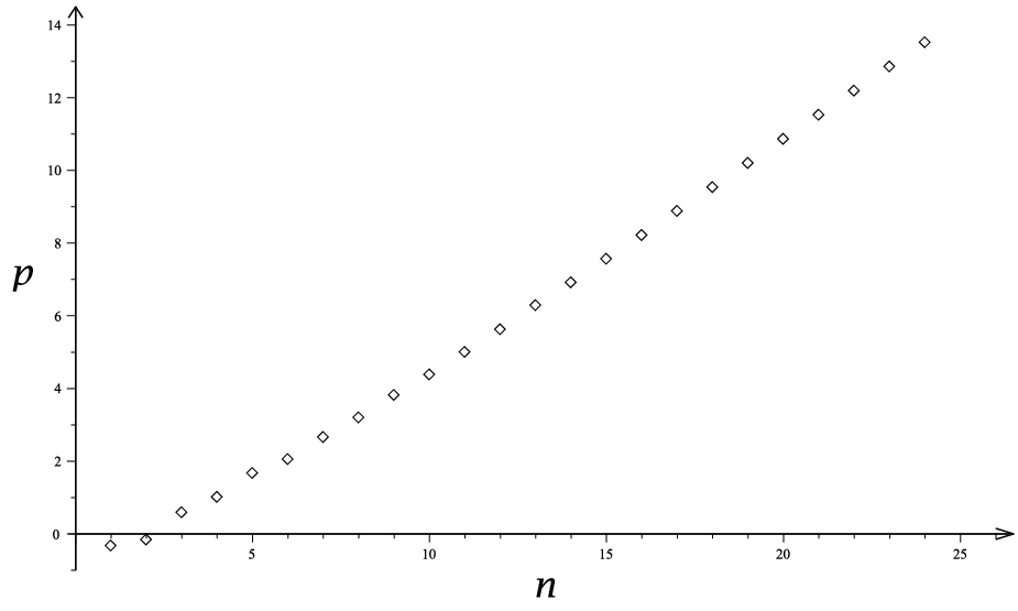
Refer to caption — Figure 1: Plot of $2^{n}(p_{n}^{rand,opt}-2/3)$ .

We can similarly ask how much of a reduction in winning probabilities Player II incurs when employing a random strategy instead of playing optimally. Table 7 shows the winning probabilities for Player II assuming optimal play by Player I and either optimal or random play by Player II. As can be seen from this table, the difference between an optimal strategy and a random strategy is far more dramatic for Player II than it is for Player I: Under random play, Player II’s winning probabilities decrease from just below $2/3$ to just below $1/2$ .

$n$	$p_{n}^{opt,opt}$	$p_{n}^{opt,rand}$	$2^{n}(1/2-p_{n}^{opt,rand})/n$
5	0.65384615	0.46497915	0.22413343
6	0.66000000	0.47844501	0.22991993
7	0.66326531	0.48728813	0.23244566
8	0.66494845	0.49267595	0.23436966
9	0.66580311	0.49585625	0.23573334
10	0.66623377	0.49768613	0.23694059
11	0.66644993	0.49872187	0.23796489
12	0.66655823	0.49930014	0.23888612
13	0.66661243	0.49961965	0.23967636
14	0.66663954	0.49979460	0.24038122
15	0.66665310	0.49988968	0.24100430
16	0.66665989	0.49994103	0.24155677
17	0.66666328	0.49996861	0.24204743
18	0.66666497	0.49998335	0.24248627
19	0.66666582	0.49999120	0.24287996
20	0.66666624	0.49999536	0.24323508
21	0.66666645	0.49999756	0.24355672
22	0.66666656	0.49999872	0.24384934
23	0.66666661	0.49999933	0.24411662
24	0.66666664	0.49999965	0.24436169

Table 7: Optimal versus random play by Player II.

The last column of Table 7 suggests a more precise asymptotic formula for $p_{n}^{opt,rand}$ , stated in the following conjecture.

Conjecture 7.2.

The probability $p_{n}^{opt,rand}$ that Player II wins assuming optimal play by Player I and random play by Player II satisfies

\frac{1}{2}-p_{n}^{opt,rand}\sim\frac{1}{4}\frac{n}{2^{n}}\quad(n\to\infty).

(7.5)

Optimal strategy for Player II in the flipped game.

For the flipped Penney-Ante game in which the player whose string appears last wins we determined in Theorem 4 all optimal strategies for Player I. It is natural to ask what the optimal strategies for Player II are in such a flipped game. In analogy to the standard Penney-Ante game, a reasonable guess might be that, given a string selected by Player I, Player II has a unique optimal response string consisting of the suffix of length $n-1$ of the string chosen by Player I followed by either an $H$ or a $T$ . However, Table 8 shows that, while such strings generally do perform well in the flipped game, they are not always optimal, and that the optimal response string is not always unique.

String	Best Response String(s)	Probability
HHHHH	HHHHH, HHHHT, TTTTT	$1/2$
HHHHT	TTTTT	$31/46$
HHHTH	HHTHH, HHTHT	$2/3$
HHHTT	TTTTT	$31/44$
HHTHH	HHHHH	$7/11$
HHTHT	HTHTH	$10/13$
HHTTH	HTTHT	$9/13$
HHTTT	TTTTT	$31/40$
HTHHH	HHHHH	$3/4$
HTHHT	THHTT	$17/26$
HTHTH	HHHHH	$3/5$
HTHTT	THTTH, THTTT	$17/24$
HTTHH	HHHHH	$15/22$
HTTHT	TTTTT	$31/48$
HTTTH	HHHHH	$15/23$
HTTTT	TTTTT	$31/32$

Table 8: Best response strings, and the corresponding win probabilities, in the flipped Penney-Ante game for strings of length

5

Note that in each case in Table 8, the optimal response strings are either of the form $HH\dots H$ , $TT\dots T$ , or consist of the last $n-1$ bits of the string chosen by Player I followed by an $H$ or $T$ . Computer calculations show that this pattern persists at least up to $n=10$ , thus suggesting the following conjecture.

Conjecture 7.3.

Assume Player I chooses a string $A=a_{1}\dots a_{n}$ . Then the best response strings for Player II in the flipped Penney-Ante game are one or more of the following four strings:

HH\dots H,\quad TT\dots T,\quad a_{2}\dots a_{n}H,\quad a_{2}\dots a_{n}T.

(7.6)

References

[1] G. Blom and D. Thorburn, How many random digits are required until given sequences are obtained?, J. Appl. Probab. 19 (1982), 518–531.
[2] S. Breen, M. S. Waterman, and N. Zhang, Renewal theory for several patterns, J. Appl. Probab. 22 (1985), 228–234.
[3] R. Chen and A. Zame, On fair coin-tossing games, J. Multivariate Anal. 9 (1979), 150–156.
[4] J. A. Csirik, Optimal strategy for the first player in the Penney Ante game, Combin. Probab. Comput. 1 (1992), 311–321.
[5] D. Felix, Optimal Penney Ante strategy via correlation polynomial identities, Electron. J. Combin. 13 (2006), R35.
[6] M. Gardner, On the paradoxical situations that arise from nontransitive relations, Scientific American 231 (1974), no. 4, 120–125.
[7] L. J. Guibas and A. M. Odlyzko, String overlaps, pattern matching, and nontransitive games, J. Combin. Theory Ser. A 30 (1981), 183–208.
[8] S.-Y. Li, A martingale approach to the study of occurrence of sequence patterns in repeated experiments, Ann. Probab. 8 (1980), 1171–1176.
[9] J. Noonan and D. Zeilberger, The Goulden-Jackson cluster method: extensions, applications and implementations, J. Differ. Equations Appl. 5 (1999), 355–377.
[10] OEIS Foundation Inc., The On-Line Encyclopedia of Integer Sequences, http://oeis.org, 2020.
[11] W. Penney, Problem 95: Penney-Ante, J. Recreat. Math. 7 (1974), 321.
[12] V. Pozdnyakov and M. Kulldorff, Waiting times for patterns and a method of gambling teams, Amer. Math. Monthly 113 (2006), 134–143.

1 Introduction and Statement of Results

The Penney-Ante Game.

Optimal strategy for Player II.

Optimal strategies for Player I.

The number of optimal strategies for Player I.

Theorem 1.

Theorem 2.

Theorem 3.

Optimal strategies in the “flipped” Penney-Ante game.

Theorem 4.

Outline of the paper.

2 Conway Numbers and Conway’s Algorithm

Definition 2.1 (Conway numbers).

Example 2.2.

Proposition 2.3 (Conway’s Algorithm).

Lemma 2.4.

Proof.

Lemma 2.5.

Proof.

3 Proof of Theorem 1

Proposition 3.1 (Csirik [4, Corollary 4]).

Corollary 3.2.

Proof.

Proof of (3.4).

Proof of (3.5).

4 Proof of Theorem 2

Lemma 4.1.

Proof.

Lemma 4.2.

Proof.

Lemma 4.3.

Proof.

Proof of Theorem 2.

5 Proof of Theorem 3

Lemma 5.1.

Proof.

Proof of Theorem 3.

6 Proof of Theorem 4

Lemma 6.1.

Proof.

7 Open Problems and Conjectures

Arithmetic nature of α\alpha.

Winning probabilities under random instead of optimal strategies.

Conjecture 7.1.

Conjecture 7.2.

Optimal strategy for Player II in the flipped game.

Conjecture 7.3.

References

Arithmetic nature of $\alpha$ .