Adaptive BEM for elliptic PDE systems,
part II: Isogeometric analysis
with hierarchical B-splines
for weakly-singular integral equations
Abstract.
We formulate and analyze an adaptive algorithm for isogeometric analysis with hierarchical B-splines for weakly-singular boundary integral equations. We prove that the employed weighted-residual error estimator is reliable and converges at optimal algebraic rate. Numerical experiments with isogeometric boundary elements for the 3D Poisson problem confirm the theoretical results, which also cover general elliptic systems like linear elasticity.
Key words and phrases:
boundary element method; isogeometric analysis; hierarchical splines; adaptivity; optimal convergence2010 Mathematics Subject Classification
65D07, 65N12, 65N15, 65N38, 65N501. Introduction
1.1. State of the art
The central idea of isogeometric analysis (IGA) is to use the same ansatz functions for the discretization of the partial differential equation (PDE) at hand, as are used for the representation of the problem geometry. Usually, the problem geometry is represented in computer aided design (CAD) by means of non-uniform rational B-splines (NURBS), T-splines, or hierarchical splines. This concept, originally invented in [HCB05] for finite element methods (IGAFEM) has proved very fruitful in applications; see also the monograph [CHB09].
Usually, CAD programs only provide a parametrization of the boundary instead of the domain itself. In particular, for isogeometric FEM, the parametrization needs to be extended to the whole domain , which is non-trivial and still an active research topic. The boundary element method (BEM) circumvents this difficulty by working only on the CAD provided boundary . However, compared to the IGAFEM literature, only little is found for isogeometric BEM (IGABEM). Based on a collocation approach, the latter was first considered in [PGK+09] for 2D and in [SSE+13] for 3D. We refer to the monograph [BMD20] for an introduction on IGABEM and to [DHK+18, DHK+20] for an efficient IGABEM implementation based on the fast multipole method. However, to the best of our knowledge, a posteriori error estimation and adaptive mesh-refinement for IGABEM, have only been considered for simple 2D model problems in the own works [FGP15, FGHP16, FGHP17, FGPS19, GPS20], which employ B-splines on the one-dimensional boundary, and the recent work [FGK+19], which employs hierarchical B-splines. In particular, [FGP15] also appears to be the first work that considers Galerkin IGABEM.
For standard BEM with (dis)continuous piecewise polynomials, a posteriori error estimation and adaptive mesh-refinement are well understood. We refer to [FFH+15] for an overview on available a posteriori error estimation strategies. Moreover, optimal convergence of mesh-refining adaptive algorithms has been proved for polyhedral boundaries [FFK+14, FFK+15, FKMP13] as well as smooth boundaries [Gan13]. The work [AFF+17] allows to transfer these results to piecewise smooth boundaries; see also the discussion in the review article [CFPP14].
In the frame of adaptive IGAFEM, a rigorous error and convergence analysis is first found in [BG16b], which proves linear convergence for some adaptive IGAFEM with hierarchical splines for the Poisson equation. Optimal algebraic rates have been proved independently from each other in [BG17, GHP17] for IGAFEM with (truncated) hierarchical B-splines. In particular, [GHP17] especially identified certain abstract properties on the mesh-refinement and the used ansatz spaces that automatically guarantee optimal convergence. In [GP20b], we have recently verified these properties for IGAFEM with T-splines as well.
Unlike adaptive IGAFEM, the rigorous error and convergence analysis of adaptive IGABEM is completely open beyond the 2D results mentioned above and thus the focus of the present work. In Part 1 of this work [GP20a], we followed the idea of [GHP17] and identified an abstract framework, which guarantees optimal convergence of adaptive BEM for weakly-singular integral equations. In the present work (Part 2), we now show that IGABEM with hierarchical splines is indeed covered by this abstract framework.
1.2. Outline
The remainder of this manuscript is roughly organized as follows: Section 2 recalls conforming BEM for weakly-singular integral equations; see (2.17) for the precise model problem. Section 3 defines hierarchical meshes and hierarchical splines on the boundary and introduces some local mesh-refinement rule (Algorithm 3.7) which preserves admissibility in the sense of a certain mesh-grading property. The main result of Section 3 is Theorem 3.10, which states reliability (3.48) of the weighted-residual error estimator (3.43) as well as linear convergence (3.49) with optimal algebraic rates (3.50) of a standard adaptive algorithm (Algorithm 3.9) applied to the model problem at hand. Remark 3.13 extends the result to rational hierarchical splines. The proof of Theorem 3.10 (and Remark 3.13) is given in Section 5, which recalls the abstract framework from [GP20a] and subsequently verifies the corresponding properties in the considered isogeometric setting. Two numerical experiments in Section 4 underpin the theoretical results, but also demonstrate the limitations of hierarchical splines in the frame of adaptive BEM when the solution exhibits edge singularities.
2. Preliminaries
In this section, we fix some general notation, recall Sobolev spaces on the boundary, and precisely state the considered problem. Throughout the work, let be a bounded Lipschitz domain as in [McL00, Definition 3.28] with boundary .
2.1. General notation
Throughout and without any ambiguity, denotes the absolute value of scalars, the Euclidean norm of vectors in , and the Hausdorff measure of any - or lower-dimensional set in . Let denote the open ball around with radius . For , let . Moreover, let and . We write to abbreviate with some generic constant , which is clear from the context. Moreover abbreviates . Throughout, mesh-related quantities have the same index, e.g., is the ansatz space corresponding to the mesh . The analogous notation is used for meshes , etc.
2.2. Sobolev spaces
For , we define the Hilbert spaces as in [McL00, page 99] by use of Bessel potentials on and liftings via bi-Lipschitz mappings11 1 For and , a mapping is bi-Lipschitz if it is bijective and as well as its inverse are Lipschitz continuous. that describe . For , it holds that with equivalent norms. We set .
For , any measurable subset , and all , we define the associated Sobolev–Slobodeckij norm
| (2.1) |
It is well-known that provides an equivalent norm on ; see, e.g., [Ste08, Lemma 2.19] and [McL00, Theorem 3.30 and page 99] for and [ME14, Theorem 2.28] for . Here, denotes the usual (weak) surface gradient which can be defined for almost all as follows: Since is a Lipschitz boundary, there exist an open cover in of such that each can be parametrized by a bi-Lipschitz mapping , where is an open set. By Rademacher’s theorem, is almost everywhere differentiable. With denoting the weak Jacobian matrix, the corresponding Gram determinant is almost everywhere positive. Moreover, by definition of the space , implies that . With the weak derivative , we can hence define
| (2.2) |
This definition does not depend on the particular choice of the open sets and the corresponding parametrizations ; see, e.g., [ME14, Theorem 2.28]. With (2.2), we immediately obtain the chain rule
| (2.3) |
For , is a realization of the dual space of according to [McL00, Theorem 3.30 and page 99]. With the dual bracket , we define an equivalent norm
| (2.4) |
Moreover, we abbreviate
| (2.5) |
[McL00, page 76] states that for , where the inclusion is continuous and dense. In particular, forms a Gelfand triple in the sense of [SS11, Section 2.1.2.4] for all , where is interpreted as function in via
| (2.6) |
So far, we have only dealt with scalar-valued functions. For , , , we define . If , and is an arbitrary measurable set, we define and similarly. With the definition
| (2.7) |
it holds that . Note that with can be identified with the dual space of , where we set
| (2.8) |
As before we abbreviate
| (2.9) |
and set
| (2.10) |
2.3. Model problem
We consider a general second-order linear system of PDEs on the -dimensional bounded Lipschitz domain with partial differential operator
| (2.11) | ||||
where the coefficients are constant for some fixed dimension . We suppose that . Moreover, we assume that is coercive on , i.e., the sesquilinear form
| (2.12) |
is elliptic up to some compact perturbation. This is equivalent to strong ellipticity of the matrices in the sense of [McL00, page 119].
Let be a corresponding (matrix-valued) fundamental solution in the sense of [McL00, page 198], i.e., a distributional solution of , where denotes the Dirac delta function. For , we define the single-layer operator as
| (2.13) |
According to [McL00, page 209 and 219–220] and [HMT09, Corollary 3.38], this operator can be extended for arbitrary ] to a bounded linear operator
| (2.14) |
For , [McL00, Theorem 7.6] states that is always elliptic up to some compact perturbation. We assume that it is elliptic even without perturbation, i.e.,
| (2.15) |
For instance, this is satisfied for the Laplace problem or for the Lamé problem, where the case requires an additional scaling of the geometry ; see, e.g., [Ste08, Chapter 6]. We stress that is not necessarily self-adjoint; see [McL00]. The sesquilinear form is continuous due to (2.14), i.e., it holds with that
| (2.16) |
Given a right-hand side , we consider the boundary integral equation
| (2.17) |
Such equations arise from the solution of Dirichlet problems of the form in with on for some ; see, e.g., [McL00, page 226–229] for more details. The Lax–Milgram lemma provides existence and uniqueness of the solution of the equivalent variational formulation of (2.17)
| (2.18) |
In particular, we see that is an isomorphism. In the Galerkin boundary element method, the test space is replaced by some discrete subspace . Again, the Lax–Milgram lemma guarantees existence and uniqueness of the solution of the discrete variational formulation
| (2.19) |
and can in fact be computed by solving a linear system of equations. We note the Galerkin orthogonality
| (2.20) |
along with the resulting Céa-type quasi-optimality
| (2.21) |
3. Boundary element method with hierarchical splines
In this section, we consider with . We introduce hierarchical splines on the boundary and propose a local mesh-refinement strategy. To this end, we assume the existence of a mesh of , i.e., with interfaces having -dimensional measure zero for , such that each surface can be parametrized over . We formulate an adaptive algorithm (Algorithm 3.9) for conforming BEM discretizations of our model problem (2.17), where adaptivity is driven by the residual a posteriori error estimator (see (3.43) below). The main result of this section is Theorem 3.10, which states that the employed estimator is reliable and converges linearly at optimal rate. The proof of Theorem 3.10 is given in Section 5.
3.1. Parametrization of the boundary
We assume that for all , the surface can be parametrized via a bi-Lipschitz mapping
| (3.1) |
where . In particular, is almost everywhere differentiable, and there exists a constant such that
| (3.2a) | |||
| and the Gram determinant satisfies that | |||
| (3.2b) | |||
see, e.g., [Gan17, Lemma 5.2.1]. We define the set of nodes
| (3.3) |
We suppose that there are no (initial) hanging nodes, i.e., the intersection with is either empty or a common (transformed) lower-dimensional hyperrectangle , where and with and the linear spans of at most of the unit vectors . Moreover, with the node patch for , we suppose the following compatibility assumption for the different parametrizations: For all nodes , there exists a polytope , i.e., an interval for , a polygon for , and a polyhedron for , and a bi-Lipschitz mapping
| (3.4) |
such that is an affine bijection for all with . Put into words, this means that each node patch can be flattened, where the corresponding bi-Lipschitz mapping restricted to any contained surface essentially coincides with the parametrization . In particular, this prohibits the case . The same assumption is also made in [SS11, Assumption 4.3.25] for curvilinear triangulations. It particularly implies that the parametrizations essentially coincide at the boundary of the surfaces, i.e., for all with non-empty intersection , it holds that
| (3.5) |
where is an affine bijection. By possibly enlarging from (3.2), we can assume that
| (3.6) |

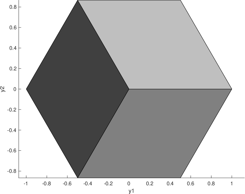

3.2. Uniformly refined tensor meshes and tensor-product splines
For , let be a vector of fixed polynomial degrees in , and set
| (3.7) |
Let
| (3.8) |
be a fixed initial -dimensional vector of -open knot vectors, i.e.,
| (3.9) |
for (in ) monotonously increasing knots such that and . Additionally, we suppose for the multiplicity (within the knot vector ) of all interior knots that
| (3.10) |
For each , this yields the corresponding mesh on
| (3.11) |
and the corresponding splines on
| (3.12) | ||||
The so-called B-splines form a basis of the latter space
| (3.13) |
see Figure 3.2 for an illustrative example. For convenience of the reader, we recall the following definition of B-splines via divided differences22 2 For any (sufficiently smooth) function and arbitrary points , divided differences are recursively defined via and if and else for .,
see also [dB01] for equivalent definitions and elementary properties. We only mention that each B-spline is positive on and vanishes outside of . Finally, we define the tensor mesh on
| (3.14) |
and the tensor-product splines
| (3.15) |
A corresponding basis is given by the set of tensor-product B-splines
| (3.16) | ||||

For , we set and recursively define for as the uniform -refinement of
| (3.17) |
i.e., it is obtained by inserting the midpoint of any non-empty knot span with multiplicity one to the knots . In particular, the old knots are not changed in . Replacing the index by , one can define the corresonding meshes, splines, and B-splines , , , , , as before. This yields a nested sequence of tensor-product spline spaces
| (3.18) |
where the last relation follows from the assumption for the multiplicity of the interior knots.
Remark 3.1.
We define the nested sequence of tensor-product spline spaces in the most simple way. Another natural approach is to use uniform -refinement with knots of some fixed multiplicities for as in [Gan17, Remark 3.4.1] instead of multiplicity one. The choice for all , that we consider, leads to the highest possible regularity of the splines at newly inserted mesh lines, whereas the maximal choice only leads to continuity at new mesh lines. In particular, if all interior knots of the initial knots already have multiplicity , the latter choice leads to the space of all continuous -piecewise tensor-product polynomials of degree .
3.3. Hierarchical meshes and splines on the parameter domains
Let . We say that a set
| (3.19) |
is a hierarchical mesh on the parameter domain if it is a partition of in the sense that , where the intersection of two different elements with has (-dimensional) measure zero. Since for with , we can define for an element ,
| (3.20) |
For an illustrative example of a hierarchical mesh, see Figure 3.3. In particular, any uniformly refined tensor mesh with is a hierarchical mesh.
For a hierarchical mesh , we define a corresponding nested sequence of closed subsets of by
| (3.21) |
It holds that
| (3.22) |
Indeed, in the literature, one usually assumes that one is given the sequence and defines the corresponding hierarchical mesh via (3.22). Note that, for , is the unique integer with and . With this, we can define the corresponding hierarchical B-splines on the parameter domain
| (3.23) |
The space of (-dimensional) hierarchical splines on the parameter domain is just defined as the product of the resulting span
| (3.24) |
It is easy to check that if is a tensor mesh and hence coincides with some , then the hierarchical basis and the standard tensor-product B-spline basis are the same. Thus, the notation is consistent with the notation from (3.16). One can prove that is linearly independent; see, e.g., [VGJS11, Lemma 2]. Since for , we can define for a basis function
| (3.25) |
Note that is the unique integer with and .

The hierarchical basis and the mesh are compatible in the sense that
| (3.26) |
see, e.g., [GHP17, Section 3.2] for the elementary argumentation.
Finally, we say that a hierarchical mesh is finer than if is obtained from via iterative dyadic bisection. Formally, this can be stated as for all . In this case, the corresponding hierarchical spline spaces are nested according to [VGJS11, Proposition 4], i.e.,
| (3.27) |
For a more detailed introduction to hierarchical meshes and splines, we refer to, e.g., [VGJS11, GJS12, BG16a, SM16].
3.4. Admissible hierarchical meshes on the parameter domains
We recall the definition and some properties of admissible meshes introduced in [GHP17, Section 3.5]. Let and be an arbitrary hierarchical mesh on . We define the set of all neighbors of an element as
| (3.28) |
The following lemma from [GHP17, Lemma 5.2] provides a relation between the set of neighbors and the patch of an element .
Lemma 3.2.
There holds that
| (3.29) |
where .
We call admissible if
| (3.30) |
Let be the set of all admissible hierarchical meshes on . Clearly, all tensor meshes , , belong to . Moreover, admissible meshes satisfy the following interesting properties, which are also important for an efficient implementation of finite or boundary element methods with hierarchical splines; see [GHP17, Proposition 3.2] for a proof.
Proposition 3.3.
For each , the support of any hierarchical B-spline is the union of at most elements . Moreover, for any , there are at most basis functions with support on , i.e., .
Remark 3.4.
(a) Since the support of any is connected, Proposition 3.3 particularly shows that for some element implies that , where is recursively defined via and for .
(b) [BG16b] studied related admissible hierarchical meshes. Whereas our admissibility is chosen such that Proposition 3.3 holds for hierarchical B-splines, their weaker definition of admissibility only guarantees Proposition 3.3 for truncated hierarchical B-splines; see [GHP17, Remark 3.2]. We also note that our admissibility guarantees Proposition 3.3 for both standard and truncated hierarchical B-splines. This follows immediately from (5.21) below. Moreover, the computation of the truncated hierarchical B-splines simplifies greatly on our admissible meshes; see [GHP17, Proposition 5.2].
Remark 3.5.
For , Lemma 3.2 immediately yields that
| (3.31) |
We note that in the proof of Lemma 3.2, one exploits that all interior knot multiplicities are smaller or equal than the corresponding polynomial degree . Actually, this is the only place, where we need this assumption, since we do not require continuous ansatz functions to discretize . However, this lemma is of course essential as it implies for example local quasi-uniformity (3.31) for admissible meshes. If one drops the additional assumption on the knot multiplicities and allows multiplicities up to as well as lowest-order polynomial degrees , one could define the neighbors of an element in an arbitrary hierarchical mesh differently as
| (3.32) |
and adapt the definition of admissibility. Then, Lemma 3.2 and Proposition 3.3 remain valid. Moreover, newly inserted knots can also have multiplicity , i.e., the choice in Remark 3.1 is possible.
3.5. (Admissible) hierarchical meshes and splines on the boundary
In order to transform the definitions from the parameter domain to the boundary part , we use the parametrizations from Section 3.1. All previous definitions can now also be made on each part , just by pulling them from the parameter domain via the bi-Lipschitz mapping . For these definitions, we drop the symbol . If is a hierarchical mesh in the parameter domain , we define the corresponding mesh on as . In particular, we have that . Moreover, let denote the set of all admissible meshes on , where is the set of all admissible hierarchical meshes on . For an arbitrary hierarchical mesh on , we introduce the corresponding hierarchical spline space
| (3.33) |
Finally, it remains to define hierarchical meshes and splines on itself. This can be done by gluing the previous definitions for the single surfaces together. For all , let be a hierarchical mesh on . We define the corresponding hierarchical mesh on by . For , we denote . We call admissible if the mesh satisfies the following two properties:
- •
All partial meshes are admissible, i.e., for all .
- •
There are no hanging nodes on the boundary of the surfaces , i.e., the intersection for with is either empty or a common (transformed) lower-dimensional hyperrectangle.
We define the set of all admissible hierarchical meshes on as , and suppose that the initial mesh on is admissible, i.e.,
| (3.34) |
For an arbitrary hierarchical mesh on , the corresponding hierarchical splines read
| (3.35) |
Remark 3.6.
(a) The property that there are no hanging nodes implies local quasi-uniformity at the boundaries , i.e., if with have non-empty intersection , then . Indeed, the intersection of is either empty or a common (transformed) lower-dimensional hyperrectangle. Thus, if , then . If , i.e., if is only a point, there exists a sequence of elements with and such that and for all . The previous argumentation yields that .
(b) Since, the ansatz space only needs to be a subset of , the property that there are no hanging nodes can actually be replaced by local quasi-uniformity at the boundaries as in (a), which is sufficient for the following analysis. However, for the hyper-singular integral equation which appears for the Neumann problem in with conormal derivative on for some given (see, e.g., [McL00, pages 229–231]), the ansatz functions must be in . In this case, the natural choice for the ansatz space is , which is even a subset of . If one supposes that there are no hanging nodes, one can define a local basis with the help of [GHP17, Proposition 3.1], which states that hierarchical B-splines on restricted onto any hyperface of are hierarchical B-splines on . The knowledge of such a basis is not only essential for an efficient implementation, but is also needed, e.g., for the definition of a quasi-interpolation operator.
3.6. Refinement of hierarchical meshes
In this section, we present a concrete refinement algorithm to specify the setting of Section 5.2. We start in the parameter domain. Recall that a hierarchical mesh is finer than another hierarchical mesh if for all . Then, is obtained from by iterative dyadic bisections of the elements in . To bisect an element , one just has to add it to the set ; see (3.42) below. In this case, the corresponding spaces are nested according to (3.27). To transfer this definition onto the surface for , we essentially just drop the symbol . We say that a hierarchical mesh on is finer than another hierarchical mesh on , if the corresponding meshes in the parameter domain satisfy this relation, i.e., if is finer than . In this case, it holds that
| (3.36) |
Finally, we call a hierarchical mesh on finer than another hierarchical mesh on , if the corresponding partial meshes satisfy this relation, i.e., if is finer than for all . In this case, it holds that
| (3.37) |
Let be a hierarchical mesh and , i.e., for some . Let be the corresponding element in the parameter domain. We define the sets of neighbors
| (3.38) |
where is the set from (3.28), and
| (3.39) |
Further, we define the sets of bad neighbors
| (3.40) |
where , and
| (3.41) | ||||
Algorithm 3.7.
Input: Hierarchical mesh , marked elements .
- (i)
Iterate the following steps (a)–(b) for until :
- (a)
Define .
- (b)
Define .
- (a)
- (ii)
Dyadically bisect all in the parameter domain by adding the corresponding to the set and obtain a finer hierarchical mesh , where for all and all
(3.42)
Output: Refined mesh .
Clearly, is finer than . For any hierarchical mesh on , we define as the set of all hierarchical meshes on such that there exist hierarchical meshes and marked elements with , and . Note that , which is why . The following proposition characterizes the set . In particular, it shows that . The proof works as for IGAFEM in [GHP17, Proposition 5.1], where the assertion is stated for ; see [Gan17, Proposition 5.4.3] for further details.
Proposition 3.8.
If , then coincides with the set of all admissible hierarchical meshes that are finer than .
3.7. Error estimator
Let . Due to the regularity assumption , the mapping property (2.14), and , the residual satisfies that for all . This allows to employ the weighted-residual a posteriori error estimator
| (3.43a) | |||
| where, for all , the local refinement indicators read | |||
| (3.43b) | |||
This estimator goes back to the works [CS96, Car97], where reliability (3.48) is proved for standard 2D BEM with piecewise polynomials on polygonal geometries, while the corresponding result for 3D BEM is first found in [CMS01].
3.8. Adaptive algorithm
We consider the following concrete realization of the abstract algorithm from, e.g., [CFPP14, Algorithm 2.2].
Algorithm 3.9.
Input:
Dörfler parameter and marking constant .
Loop: For each , iterate the following steps:
- (i)
Compute Galerkin approximation .
- (ii)
Compute refinement indicators for all elements .
- (iii)
Determine a set of marked elements which has up to the multiplicative constant minimal cardinality, such that the following Dörfler marking is satisfied
(3.44) - (iv)
Generate refined mesh .
Output: Refined meshes and corresponding Galerkin approximations with error estimators for all .
3.9. Optimal convergence
We set
| (3.45) |
and, for all ,
| (3.46) |
We say that the solution lies in the approximation class with respect to the estimator if
| (3.47) |
By definition, implies that the error estimator on the optimal meshes decays at least with rate . The following main theorem of our work states that each possible rate will indeed be realized by Algorithm 3.9. The proof is given in Section 5. There, we will verify certain abstract properties to employ our recent abstract counterpart [GP20a, Theorem 3.4] of Theorem 3.10, which itself builds on the so-called axioms of adaptivity from [CFPP14]. Such an optimality result was first proved in [FKMP13] for the Laplace operator on a polyhedral domain . As ansatz space, [FKMP13] considered piecewise constants on shape-regular triangulations. [FFK+14] in combination with [AFF+17] extends the assertion to piecewise polynomials on shape-regular curvilinear triangulations of some piecewise smooth boundary . Independently, [Gan13] proved the same result for globally smooth and arbitrary symmetric and elliptic boundary integral operators.
Theorem 3.10.
Let be the sequence of meshes generated by Algorithm 3.9. Then, there hold the following statements (i)–(iii):
- (i)
The residual error estimator (3.43)satisfies reliability, i.e., there exists a constant such that
(3.48) - (ii)
For arbitrary and , the estimator converges linearly, i.e., there exist constants and such that
(3.49) - (iii)
There exists a constant such that for all and , the estimator converges at optimal rate, i.e., for all , there exist constants such that
(3.50)
All involved constants , and depend only on the dimensions , the coefficients of the differential operator , the boundary , the (fixed) number of boundary parts , the parametrizations and , the initial meshes , and the polynomial orders for and (see (3.3)), while depend additionally on and the sequence , and depends furthermore on and . The constant depends only on , , , and if there exists with , then also on and .
Remark 3.11.
If the sesquilinear form is Hermitian, then , and are independent of ; see [GP20a, Remark 4.14].
Remark 3.12.
Under the assumption that as , one can show that ; see [GP20a, Remark 3.7] for the elementary proof. This observation allows to follow the ideas of [BHP17] and to show that the adaptive algorithm yields optimal convergence even if the sesquilinear form is only elliptic up to some compact perturbation, provided that the continuous problem is well-posed. This includes, e.g., adaptive BEM for the Helmholtz equation; see [Ste08, Section 6.9]. For details, the reader is referred to [BHP17, BBHP19].We note that can easily be algorithmically enforced (without influencing the optimality result) by additionally marking the largest elements in Algorithm 3.9 (iii); see [BHP17, Proposition 16].
Remark 3.13.
(a) Theorem 3.10 is still valid if one replaces the ansatz space by rational hierarchical splines, i.e., by the set
| (3.51) |
where is a fixed positive weight function in the initial space of hierarchical splines for all . With the B-spline basis on , we even suppose that can be written as
| (3.52) |
We will prove this generalization in Section 5.4. In this case, the constants depend additionally on .
(b) Moreover, Theorem 3.10 still holds true if newly inserted knots have a multiplicity higher than one, i.e., if one uses the uniformly refined knots of Remark 3.1 with to define (rational) hierarchical splines. The corresponding proof works verbatim.
(c) Finally, if one defines for an element of a hierarchical mesh its neighbours as in Remark 3.5, and adapts the definition of admissibility and accordingly, one can also allow for lowest-order polynomial degrees as well as full knot multiplicities .
4. Numerical experiments with hierarchical splines
In this section, we empirically investigate the performance of Algorithm 3.9 in two typical situations: In Section 4.1, the solution is generically singular at the edges of . In Section 4.2, the solution is nearly singular at one point. We consider the 3D Laplace operator . The corresponding fundamental solution reads
| (4.1) |
As already mentioned in Section 2.3, the corresponding single-layer operator is elliptic. For experiments in 2D, we refer to the recent work [FGK+19] for univariate hierarchical splines and to [FGHP16, FGPS19, GPS20] for univariate standard and rational splines.
In the first example (Section 4.1), we consider the exterior Laplace–Dirichlet problem
| (4.2a) | ||||
| for given Dirichlet data , together with the radiation condition | ||||
| (4.2b) | ||||
Then, (4.2) can be equivalently rewritten as integral equation (2.17); see, e.g., [McL00, Theorem 7.15 and Theorem 8.9]. Indeed, the (exterior) normal derivative of the weak solution of (4.2) satisfies the integral equation (2.17) with , i.e.,
| (4.3) |
where
| (4.4) |
denotes the double-layer operator. According to [SS11, Corollary 3.3.12 and Theorem 3.3.13], if is piecewise smooth and if , there holds the representation
| (4.5) | ||||
In the second example (Section 4.2), we consider the interior Laplace–Dirichlet problem
| (4.6) | ||||
for given Dirichlet data . Then, (4.6) can be equivalently rewritten as integral equation (2.17); see, e.g., [McL00, Theorem 7.6]. Indeed, the normal derivative of the weak solution of (4.6) satisfies the integral equation (2.17) with and the double-layer operator (4.4), i.e.,
| (4.7) |
The integral representation (4.5) is satisfied for both examples. Indeed, the surfaces of the boundary are parametrized via rational splines, i.e., for each , there exist polynomial orders , a two-dimensional vector of -open knot vectors with multiplicity smaller or equal to for the interior knots, and a positive spline weight function such that the parametrization satisfies that
| (4.8) |
Based on the knots for the geometry, we choose the initial knots for the discretization. As basis for the considered ansatz spaces of (non-rational) hierarchical splines, we use the basis given in (5.24). To (approximately) calculate the Galerkin matrix and the right-hand side vector, we proceed as in [SS11, Chapter 5] where all singular integrals are transformed via Duffy transformations and then computed with tensor Gauss quadrature. To calculate the weighted-residual error estimator33 3 To ease the computation, we replace in (3.43) by the equivalent term . Here, denotes the corresponding element of in the parameter domain . (3.43), we employ formula (2.2) for the surface gradient and use again tensor Gauss quadrature. To this end, we approximate on an element by the gradient of the polynomial interpolation of the residual as in [Kar12, Section 7.1.5]. In particular, we have to evaluate the residual at some quadrature points which can be done (approximately) using appropriate Duffy transformations and tensor Gauss quadrature as in [Gan14, Sections 5.1–5.2].
To (approximately) calculate the energy error, we proceed as follows: Let be the Galerkin approximation of the -th step with the corresponding coefficient vector . Further, let be the Galerkin matrix. With Galerkin orthogonality (2.20) and the energy norm obtained by Aitken’s -extrapolation, we can compute the energy error as
| (4.9) | ||||
4.1. Solution with edge singularities on cube
In the first experiment, we consider
| (4.10) |
Each of the six faces of can be parametrized by non-rational splines of degree corresponding to the knot vectors ; see [GHP17, Section 6.1]. We choose the right-hand side in (2.17). Note that the constant function satisfies the Laplace problem, which is why (4.7) implies that . We conclude that
| (4.11) |
This means that the considered integral equation stems from an exterior Laplace–Dirichlet problem (4.2). In particular, we expect singularities at the non-convex edges of , i.e., at all edges of the cube .


We consider polynomial degrees . For the initial ansatz space with spline degree for all , we choose the initial knot vectors for all , where the multiplicity of and is . We choose the parameters of Algorithm 3.9 as and , where we use the refinement strategy of Remark 3.13 (c) in the lowest-order case . For comparison, we also consider uniform refinement, where we mark all elements in each step, i.e., for all . This leads to uniform bisection of all elements. In Figure 4.1, one can see some adaptively generated hierarchical meshes. In Figure 4.2 and Figure 4.3, we plot the energy error and the error estimator against the number of elements . All values are plotted in a double-logarithmic scale. The experimental convergence rates are thus visible as the slope of the corresponding curves. Although we only proved reliability (3.48) of the employed estimator, the curves for the error and the estimator are parallel in each case, which numerically indicates reliability and efficiency. The uniform approach always leads to the suboptimal convergence rate due to the edge singularities. Independently on the chosen polynomial degree , the adaptive approach leads approximately to the rate . For smooth solutions , one would expect the rate ; see [SS11, Corollary 4.1.34]. However, according to Theorem 3.10, the achieved rate is optimal if one uses the proposed refinement strategy and the resulting hierarchical splines. The reduced optimal convergence rate is probably due to the edge singularites. A similar convergence behavior is also witnessed in [FL07, Section 5.2] for the lowest-order case . [FL07] additionally considers anisotropic refinement which recovers the optimal convergence rate . We mention that for graded meshes the theoretical convergence rates are explicitly known on polyhedral domains; see [VPS90] or [GS18, Chapter 7].


4.2. Nearly singular solution on quarter pipe
We consider the quarter pipe
| (4.12) |
see Figure 4.4. We split the boundary into the six surfaces
, and can be parametrized by rational splines of degree corresponding to the knot vectors ; see [PT97, Chapter 8]. The affine surfaces and can be parametrized by non-rational splines of degree corresponding to the knot vectors ; see [GHP17, Section 6.1].


We prescribe the exact solution of the interior Laplace–Dirichlet problem (4.6) as the shifted fundamental solution
| (4.13) |
with . Although is smooth on , it is nearly singular at the midpoint of . We consider the corresponding integral equation (4.7). The normal derivative of reads
| (4.14) |


We consider polynomial degrees . For the initial ansatz space with spline degree for all , we choose the initial knot vectors for all , where the multiplicity of and is . We choose the parameters of Algorithm 3.9 as and , where we use the refinement strategy of Remark 3.13 (c) in the lowest-order case . For comparison, we also consider uniform refinement, where we mark all elements in each step, i.e., for all . In Figure 4.4, one can see some adaptively generated hierarchical meshes. In Figure 4.5 and Figure 4.6, we plot the energy error and the error estimator against the number of elements . All values are plotted in a double-logarithmic scale and the experimental convergence rates are visible as the slope of the corresponding curves. In all cases, the lines of the error and the error estimator are parallel, which numerically indicates reliability and efficiency. Since the solution is smooth, the uniform and the adaptive approach both lead to the optimal asymptotic convergence rate . However, is nearly singular at , which is why adaptivity yields a much better multiplicative constant.

5. Proof of Theorem 3.10
In [GP20a, Section 3], we have identified the crucial properties of the underlying meshes (see (M1)–(M5) below), the mesh-refinement (see (R1)–(R3) below), as well as the boundary element spaces (see (S1)–(S6) below) which ensure that the residual error estimator fits into the general framework of [CFPP14] and which hence guarantee reliability 3.48 and linear convergence at optimal rate (3.49)–(3.50); see [GP20a, Theorem 3.4]. The goal of this section is to recapitulate these properties and subsequently verify them for the present isogeometric setting; see also [Gan17, Section 5.2–5.3] for more details. In Section 5.4, we further briefly comment on how to verify the mentioned properties for rational hierarchical splines; see Remark 3.13.
5.1. Meshes
In [GP20a], we even considered general meshes of the boundary of the bounded Lipschitz domain in the following sense:
- (i)
is a finite set of compact Lipschitz domains on , i.e., each element has the form , where is a compact44 4 A compact Lipschitz domain is the closure of a bounded Lipschitz domain. For , it is the finite union of compact intervals with non-empty interior. Lipschitz domain in and is bi-Lipschitz.
- (ii)
covers , i.e., .
- (iii)
For all with , the intersection has -dimensional Hausdorff measure zero.
Clearly, any admissible hierarchical mesh is a mesh in this sense, where
| (5.1) |
In order to ease notation, we introduce for any mesh the corresponding mesh-width function
| (5.2) |
For , we define the patches of order inductively by
| (5.3) |
The corresponding set of elements is
| (5.4) |
To abbreviate notation, we set and . If for some , we write and , where we skip the index for as before. For , we define and , and the superscript is omitted for .
In the following Sections (5.1.1)–(5.1.5), we show the existence of constants such that the following properties are satisfied for all admissible hierarchical meshes :
- (M1)
Bounded element patch: For all , there holds that
i.e., the number of elements in a patch is uniformly bounded.
- (M2)
Local quasi-uniformity: For all , there holds that
i.e., neighboring elements have comparable diameter.
- (M3)
Shape-regularity: For all , there holds that
- (M4)
Patch centered elements: For all , there holds55 5 We use the convention . that
i.e., each element lies essentially in the center of its patch.
- (M5)
Local seminorm estimate: For all and , there holds that
The following proposition shows that (M5) is actually always satisfied. However, in general the multiplicative constant depends on the shape of the point patches. The proof is inspired by [DNPV12, Proposition 2.2], where an analogous assertion for norms instead of seminorms is found. For , we have already shown the assertion in the recent own work [FGHP16, Lemma 4.5]. For polyhedral domains with triangular meshes, it is proved in [FFME+14, Proposition 3.3] via interpolation techniques. Adapting the arguments of [FGHP16, Lemma 4.5], a detailed proof for our setting is found in [Gan17, Proposition 5.2.2].
Proposition 5.1.
Let be a bounded and connected Lipschitz domain and bi-Lipschitz. In particular, there exists a constant such that
| (5.5) |
Then, there exists a constant such that
| (5.6) |
The constant depends only on the dimension , the set , and .
5.1.1. Verification of (M1)
Let and . We split the patch as follows
If , there exists with . By admissibility, this implies that is even a common (transformed) lower-dimensional hyperrectangle of and . In particular, this leads to , where . Since , Remark 3.5 gives that . Altogether, we derive that with a constant which depends only on and .
5.1.2. Verification of (M2)
Let and with . Let with , and . If , then Remark 3.5 gives that for and . Bi-Lipschitz continuity of yields that . If , then admissibility of and Remark 3.6 give that . This implies that for and , and thus due to bi-Lipschitz continuity of and . This concludes local quasi-uniformity (M2), where the constant depends only the dimension , the constant , and the initial meshes for .
5.1.3. Verification of (M3)
Let , , and with . We abbreviate . As the refinement procedure relies on uniform bisection of an element in the parameter domain, we see that , where the hidden constants depend only on the dimension and the initial mesh . Since is bi-Lipschitz, we see that . Moreover, (3.2) shows that . Altogether, we conclude that , where the hidden constants depend only on , , and .
5.1.4. Verification of (M4)
Let , , and with . We show that there exists with , which verifies (M4).
Step 1: According to Remark 3.5 and Remark 3.6, admissibility shows that for all . Since we only use dyadic bisection, there exists an upper bound of the number of possible configurations of and depending only on the initial meshes and (an upper bound of) . In particular, this implies that , but the hidden constant still depends on (an upper bound for) . We see that it only remains to consider small elements with high level.
Step 2: In this step, we show that there exists a node (see (3.3)) and a generic constant such that and if is sufficiently high. Without loss of generality, we assume that and set . Note that . Since we assume that the surfaces have no hanging nodes, implies that for all . We abbreviate
Let be sufficiently high such that , which is possible due to (M1)–(M2). Note that this choice depends only on the dimension , the constant , and the initial meshes. With the assumption that , we derive that . The same argument proves that if .
Step 3: Due to Step 2, we may consider the set provided that is sufficiently high. Recall that for all ; see Step 1. With the assumptions for the mapping of Section 3.1, and since we only use dyadic bisection, we see that the number of possible shapes of and is uniformly bounded. In particular, there exists with . Bi-Lipschitz continuity of and Step 2 yield the existence of with such that
Together with Step 1, this concludes (M4), where the constant depends only on the dimension , the parametrizations and , and the initial meshes for and .
5.1.5. Verification of (M5)
We show that there are only finitely many reference point patches. Then, Proposition 5.1 will conclude (M5). Let and . According to Remark 3.5 and Remark 3.6, admissibility shows that for all . Since there are no hanging nodes in (see (3.3)), there exists such that . With the assumptions for the mapping of Section 3.1, and since we only use dyadic bisection, we see that the number of possible shapes of is uniformly bounded. More precisely, there exists a finite set of connected subsets such that for arbitrary and corresponding there exist and an affine bijection with
| (5.7) |
Since is bi-Lipschitz, there holds that , and we see for the mapping that
| (5.8) |
Thus, the application of Proposition 5.1 (on the interior of ) concludes (M5). The constant depends only on the dimension , the parametrizations and , and the initial meshes for and .
5.2. Mesh-refinement
In the following Section 5.2.1, we show that there exist and such that for all admissible hierarchical meshes and refinements with arbitrary marked elements , the following elementary properties (R1)–(R3) are satisfied:
- (R1)
Child estimate: It holds that
i.e., one step of refinement leads to a bounded increase of elements.
- (R2)
Parent is union of children: For all , it holds that
i.e., each element is the union of its successors.
- (R3)
Reduction of children: For all , it holds that
i.e., successors are uniformly smaller than their parent.
By induction and the definition of , one easily sees that (R2)–(R3) remain valid if is an arbitrary mesh in . In particular, (R2)–(R3) imply that each refined element is split into at least two children, which yields that
| (5.9) |
Besides (R1)–(R3), we show in Section 5.2.2–5.2.3 the following less trivial requirements (R4)–(R5) with constants :
- (R4)
Closure estimate: Let be an arbitrary sequence in such that with some for all . Then, for all , it holds that
- (R5)
Overlay property: For all , there exists a common refinement which satisfies the overlay estimate
5.2.1. Verification of (R1)–(R3)
The child estimate (R1) is trivially satisfied with since each refined element is split into exactly children. The union of children property (R2) holds by definition. Finally, the proof of (R3) works just as for IGAFEM in [GHP17, Section 5.3], where the assertion is stated for . The constant depends only on and .
5.2.2. Verification of (R4)
5.2.3. Verification of (R5)
Let . For each , let be the overlay of and , i.e.,
| (5.10) |
We have proved in [GHP17, Section 5.5] that , and that
| (5.11) |
Summing all components gives the overlay estimate
| (5.12) |
It remains to show that is a refinement of and , i.e., . Clearly, is finer than these meshes. Since Proposition 3.8 states that any finer admissible mesh can be reached via , we just have to verify admissibility of . As each is admissible, we only have to show that is a common transformed lower-dimensional hyperrectangle for all with non-empty intersection and as well as for some with . Without loss of generality, we assume that and . Further, we may assume that . Then, by definition of , there exist and with and . Obviously, and have non-empty intersection too. Thus, admissibility of shows that is a common transformed hyperrectangle. We suppose that is obtained from via iterative bisections, i.e., , and lead this to a contradiction. The intersection is only a proper subset of a transformed hyperrectangle of . Since , the same holds for instead of , i.e., is only a proper subset of a transformed hyperrectangle of . Thus, admissibility of leads to a contradiction, and we see that shares a common transformed hyperrecangle with .
5.3. Boundary element space
In the following Sections 5.3.1–5.3.5, we show the existence of constants , , and , such that the following properties (S1)–(S4) hold for all admissible hierarchical meshes with associated hierarchical spline space :
- (S1)
Inverse inequality: For all , it holds that
- (S2)
Nestedness: For all , it holds that
- (S3)
Local domain of definition: For all , all , and , it holds that
- (S4)
Componentwise local approximation of unity: For all and all , there exists some with
such that only the -th component does not vanish, i.e.,
and
Remark 5.2.
Besides (S1)–(S4), we show in Section 5.3.6 that there exist constants as well as such that for all admissible hierarchical meshes with associated hierarchical spline space and , there exists a linear operator with the following properties (S5)–(S6):
- (S5)
Local projection property. Let from (S3). For all and with , it holds that
- (S6)
Local -stability. For all and , it holds that
5.3.1. Verification of (S1)
For piecewise constants and piecewise affine functions on a triangulation of the boundary of a polyhedral domain , the inverse estimate (S1) is already found in [DFG+04, Theorem 4.7]. [GHS05, Theorem 3.6] and [Geo08, Theorem 3.9] generalized the result to arbitrary piecewise polynomials on curvilinear triangulations. In the recent own work [FGHP17, Proposition 4.1] and based on the ideas of [DFG+04], we proved (S1) for non-rational splines on a one-dimensional piecewise smooth boundary . In the proof, we derived the following abstract criterion for the ansatz functions which is sufficient for the inverse inequality (S1). Although, [FGHP17] considered only , the proof works verbatim for arbitrary dimension .
Proposition 5.3.
Let be a general mesh as in Section 5.1 which satisfies (M1)–(M5). We assume that the Lipschitz constants of the mappings are uniformly bounded, i.e., there exists a constant such that
| (5.13) |
Moreover, let satisfy the following assumption: There exists a constant , such that for all there exists a hyperrectangular subset of the interior (i.e., has the form with for some real numbers ) such that , does not change its sign on , and
| (5.14) |
where denotes the essential infimum. We further assume that the shape-regularity constants of the sets are uniformly bounded, i.e., there exists a constant such that
| (5.15) |
Then, there exists a constant such that
| (5.16) |
To apply Proposition 5.3 to hierarchical splines, we need the next elementary lemma which was proved in the recent own work [FGHP17, Proposition 4.1].
Lemma 5.4.
Let be a fixed polynomial degree. Let be a compact interval with positive length . Then, there exists a constant such that for all polynomials of degree on , there exists some interval of length such that does not change its sign on and
| (5.17) |
The constant depends only on .
Finally, we come to the proof of the inverse inequality (S1). Let be an admissible hierarchical mesh on . We recall that is a product space of transformed scalar-valued hierarchical splines. Without loss of generality, we assume that we are in the scalar case . We show that all satisfy the assumptions of Proposition 5.3 and hence conclude that . We have already seen that (M1)–(M5) are satisfied. Moreover, (5.13) is trivially satisfied since each is just the restriction of some to , where . For , we abbreviate . Due to the regularity (3.2) of the parametrizations , it is sufficient to find a uniform constant and a shape-regular hyperrectangle such that , does not change sign on , and
| (5.18) |
Indeed, one easily shows that implies that for some uniform constant ; see, e.g., [GHP17, Section 5.3]. Recall that coincides with a tensor-product polynomial . Hence, there exist polynomials of degree such that . With the notation and , we see that the latter inequality is satisfied if
| (5.19) |
We define as the interval of Lemma 5.4 corresponding to the polynomial on the interval . With the constant of Lemma 5.4, we set . Then, (5.19), and therefore (5.18) is satisfied. Moreover, one sees that , and that doesn’t change its sign on . It remains to prove shape-regularity (5.15). Since, the refinement procedure only uses uniform bisection of elements, the element is shape-regular in the sense that for all . Together with , this proves (5.15). Altogether, we conclude (S1), where the constant depends only on the dimensions , the (fixed) number of boundary parts , the parametrizations and , the initial meshes , and the polynomial orders for and .
5.3.2. Verification of (S2)
Let and . The nestedness was already stated in (3.37).
5.3.3. Bases of hierarchical splines on the boundary
In this section, we give two bases for . Since is a product space of transformed scalar-valued hierarchical splines, it is sufficient to consider . For , recall the definition of the set of hierarchical B-splines from Section 3.3, which is a basis of . Moreover, let
| (5.20) |
be the well-known linear truncation procedure; see, e.g, [GHP17, Section 5.9]. According to [GJS12, Theorem 6 and 9], the set of truncated hierarchical B-splines are an alternate basis of In general, truncated hierarchical B-splines have a smaller support than the corresponding hierarchical B-splines. Indeed, one even has the pointwise estimate
| (5.21) |
see, e.g., [GHP17, Section 5.9]. In contrast to hierarchical B-splines, truncated hierarchical B-splines form a partition of unity, i.e.,
| (5.22) |
see [GJS12, Theorem 10]. Consequently, there holds that
| (5.23) |
For , let denote the truncation transformed onto . Then, an alternate basis of is given by . If we identify functions in with their extension (by zero) in , we see that
| (5.24) |
An alternate basis of is given by .
5.3.4. Verification of (S3)
5.3.5. Verification of (S4)
Let . First, we recall that is a product space of transformed scalar-valued hierarchical splines. Without loss of generality, we assume that ; see Remark 5.2. [Fae00, Lemma 2.6] resp. [Fae02, Lemma 3.5] prove a similar version of (S4) for splines on a one-dimensional boundary resp. for certain piecewise polynomials of degree and on curvilinear triangulations of a two-dimensional boundary . There, the proof follows from direct calculations, where [Fae00, Lemma 2.6] actually only provides a proof of (S4) for splines of degree . In contrast, we will make use of the following abstract result.
Proposition 5.5.
Let . Let be a general mesh with associated space as in Section 5.1 which satisfies (M1)–(M3). Assume that there exists a finite subset which satisfies the following three properties:
- (i)
Non-negativity: Each is non-negative.
- (ii)
Locality: There is some such that for all there exists an element with .
- (iii)
Partition of unity: It holds that .
Then, (S4) is satisfied with , and the constant depends only on (M1)–(M3) and .
Proof.
5.3.6. Verification of (S5)–(S6)
Let and . Since is a product space of transformed scalar-valued hierarchical splines, we may assume without loss of generality that . For , we set . For any hierarchical B-spline , let with and , and let be the corresponding dual basis function on from [GHP17, Section 5.10], i.e.,
| (5.25) |
It is shown in [GHP17] that
| (5.26) |
We define the operator via
| (5.27) |
where
| (5.28) |
Recall that (see (5.21)), which is why clearly maps into the desired space .
We come to the verification of the properties (S5)–(S6). Let and of Section 5.3.4. Moreover, let with and with . Recall the notation . For all , there holds with the abbreviation that
Note that implies that . Due to Remark 3.4(a), implies that , where denotes the patch with respect to the mesh defined analogously as in (5.4). We abbreviate and note that . This yields that . Hence, we see that
If satisfies that , then there exists with . With , we see as before that implies that , which leads to
The right-hand side coincides with the projection operator from [SM16, Theorem 4] corresponding to the mesh applied to . Since , this yields that
This proves the local projection property (S5).
Finally, we prove local -stability (S6). Let again and with . With the notation from before, the boundedness of the Gram determinant (3.2) shows that
With (5.26), it follows as for IGAFEM in [GHP17, Lemma 5.6] (which proves local -stability for a similar operator mapping into ) that
With boundedness of the Gram determinant (3.2) and , we derive that
This concludes the proof of (S6). The constant depends only on the dimension , the constant , the initial meshes , and the polynomial orders for .
5.4. Proof of Theorem 3.10 for rational hierarchical splines
As mentioned in Remark 3.13, Theorem 3.10 is still valid if one replaces the ansatz space for by rational hierarchical splines, i.e., by the set
| (5.29) |
where is a fixed positive weight function in the initial space of hierarchical splines for all , where we additionally assume the representation (3.52). Indeed, the mesh properties (M1)–(M5) as well as the refinement properties (R1)–(R5) of Section 5 are independent of the discrete spaces. To verify the validity of Theorem 3.10 in the rational setting, it thus only remains to verify the properties (S1)–(S6) for the rational boundary element spaces.
To see the inverse estimate (S1), it is again sufficient to consider . In Section 5.3.1, we proved (S1) for by applying Proposition 5.3 for all . With the notation from Section 5.3.1, we showed that
where does not change its sign on . With , , and , this yields that, for all ,
In particular, the conditions for Proposition 5.3 are also satisfied for the functions in , which concludes (S1).
The properties (S2)–(S3) depend only on the numerator of the rational hierarchical splines and thus transfer.
For the proof of (S4), we exploit the representation (3.52) to verify the conditions of the abstract Proposition 5.5. Again, we may assume that . Let . Note that is also an element of the standard tensor-product spline space for all and . In particular, it can be written as linear combination of B-splines in . The representation (3.52) and the two-scale relation with only non-negative coefficients between bases of consecutive levels of [dB01, Section 11] yields that the corresponding coefficients are non-negative. Therefore, the preservation of coefficients property of [SM16, Theorem 1] or [GJS14, Theorem 12] implies that also the coefficients of the linear combination of in are non-negative, i.e.,
| (5.30) |
If we identify functions in with their extension (by zero) in , we can choose
As in Section 5.3.5, one sees that this choice satisfies the assumptions of Proposition 5.5.
Acknowledgement
The authors acknowledge support through the Austrian Science Fund (FWF) under grant P29096, grant W1245, and grant J4379.
References
- [AFF+17] Markus Aurada, Michael Feischl, Thomas Führer, Michael Karkulik, J. Melenk, and Dirk Praetorius. Local inverse estimates for non-local boundary integral operators. Math. Comp., 86(308):2651–2686, 2017.
- [BBHP19] Alex Bespalov, Timo Betcke, Alexander Haberl, and Dirk Praetorius. Adaptive BEM with optimal convergence rates for the Helmholtz equation. Comput. Methods Appl. Mech. Engrg., 346:260–287, 2019.
- [BG16a] Annalisa Buffa and Eduardo M. Garau. Refinable spaces and local approximation estimates for hierarchical splines. IMA J. Numer. Anal., 37(3):1125–1149, 2016.
- [BG16b] Annalisa Buffa and Carlotta Giannelli. Adaptive isogeometric methods with hierarchical splines: error estimator and convergence. Math. Models Methods Appl. Sci., 26(01):1–25, 2016.
- [BG17] Annalisa Buffa and Carlotta Giannelli. Adaptive isogeometric methods with hierarchical splines: Optimality and convergence rates. Math. Models Methods Appl. Sci., 27(14):2781–2802, 2017.
- [BHP17] Alex Bespalov, Alexander Haberl, and Dirk Praetorius. Adaptive FEM with coarse initial mesh guarantees optimal convergence rates for compactly perturbed elliptic problems. Comput. Methods Appl. Mech. Engrg., 317:318–340, 2017.
- [BMD20] Gernot Beer, Benjamin Marussig, and Christian Duenser. The Isogeometric Boundary Element Method. Springer, Cham, 2020.
- [Car97] Carsten Carstensen. An a posteriori error estimate for a first-kind integral equation. Math. Comp., 66(217):139–155, 1997.
- [CFPP14] Carsten Carstensen, Michael Feischl, Marcus Page, and Dirk Praetorius. Axioms of adaptivity. Comput. Math. Appl., 67(6):1195–1253, 2014.
- [CHB09] J. Austin Cottrell, Thomas J. R. Hughes, and Yuri Bazilevs. Isogeometric analysis: toward integration of CAD and FEA. John Wiley & Sons, New York, 2009.
- [CMS01] Carsten Carstensen, Matthias Maischak, and Ernst P. Stephan. A posteriori error estimate and -adaptive algorithm on surfaces for Symm’s integral equation. Numer. Math., 90(2):197–213, 2001.
- [CS96] Carsten Carstensen and Ernst P. Stephan. Adaptive boundary element mevthods for some first kind integral equations. SIAM J. Numer. Anal., 33(6):2166–2183, 1996.
- [dB01] Carl de Boor. A practical guide to splines. Springer, New York, 2001.
- [DFG+04] Wolfgang Dahmen, Birgit Faermann, Ivan G. Graham, Wolfgang Hackbusch, and Stefan A. Sauter. Inverse inequalities on non-quasi-uniform meshes and application to the mortar element method. Math. Comp., 73(247):1107–1138, 2004.
- [DHK+18] Jürgen Dölz, Helmut Harbrecht, Stefan Kurz, Sebastian Schöps, and Felix Wolf. A fast isogeometric bem for the three dimensional laplace-and helmholtz problems. Comput. Methods Appl. Mech. Engrg., 330:83–101, 2018.
- [DHK+20] Jürgen Dölz, Helmut Harbrecht, Stefan Kurz, M. Multerer, Sebastian Schöps, and Felix Wolf. Bembel: The fast isogeometric boundary element C++ library for Laplace, Helmholtz, and electric wave equation. SoftwareX, 11:100476, 2020.
- [DNPV12] Eleonora Di Nezza, Giampiero Palatucci, and Enrico Valdinoci. Hitchhiker’ s guide to the fractional Sobolev spaces. Bull. Sci. Math., 136(5):521–573, 2012.
- [Fae00] Birgit Faermann. Localization of the Aronszajn-Slobodeckij norm and application to adaptive boundary elements methods. Part I. The two-dimensional case. IMA J. Numer. Anal., 20(2):203–234, 2000.
- [Fae02] Birgit Faermann. Localization of the Aronszajn-Slobodeckij norm and application to adaptive boundary element methods Part II. The three-dimensional case. Numer. Math., 92(3):467–499, 2002.
- [FFH+15] Michael Feischl, Thomas Führer, Norbert Heuer, Michael Karkulik, and Dirk Praetorius. Adaptive boundary element methods: A posteriori error estimators, adaptivity, convergence, and implementation. Arch. Comput. Methods Engrg., 22:309–389, 2015.
- [FFK+14] Michael Feischl, Thomas Führer, Michael Karkulik, J. Markus Melenk, and Dirk Praetorius. Quasi-optimal convergence rates for adaptive boundary element methods with data approximation, Part I: Weakly-singular integral equation. Calcolo, 51(4):531–562, 2014.
- [FFK+15] Michael Feischl, Thomas Führer, Michael Karkulik, J. Markus Melenk, and Dirk Praetorius. Quasi-optimal convergence rates for adaptive boundary element methods with data approximation, Part II: Hyper-singular integral equation. Electron. Trans. Numer. Anal., 44:153–176, 2015.
- [FFME+14] Michael Feischl, Thomas Führer, Gregor Mitscha-Eibl, Dirk Praetorius, and Ernst P. Stephan. Convergence of adaptive BEM and adaptive FEM-BEM coupling for estimators without h-weighting factor. Comput. Meth. in Appl. Math., 14(4):485–508, 2014.
- [FGHP16] Michael Feischl, Gregor Gantner, Alexander Haberl, and Dirk Praetorius. Adaptive 2D IGA boundary element methods. Eng. Anal. Bound. Elem., 62:141–153, 2016.
- [FGHP17] Michael Feischl, Gregor Gantner, Alexander Haberl, and Dirk Praetorius. Optimal convergence for adaptive IGA boundary element methods for weakly-singular integral equations. Numer. Math., 136(1):147–182, 2017.
- [FGK+19] Antonella Falini, Carlotta Giannelli, Tadej Kanduč, Maria Lucia Sampoli, and Alessandra Sestini. An adaptive IgA-BEM with hierarchical B-splines based on quasi-interpolation quadrature schemes. Internat. J. Numer. Methods Engrg., 117(10):1038–1058, 2019.
- [FGP15] Michael Feischl, Gregor Gantner, and Dirk Praetorius. Reliable and efficient a posteriori error estimation for adaptive IGA boundary element methods for weakly-singular integral equations. Comput. Methods Appl. Mech. Engrg., 290:362–386, 2015.
- [FGPS19] Thomas Führer, Gregor Gantner, Dirk Praetorius, and Stefan Schimanko. Optimal additive Schwarz preconditioning for adaptive 2D IGA boundary element methods. Comput. Methods Appl. Mech. Engrg., 351:571–598, 2019.
- [FKMP13] Michael Feischl, Michael Karkulik, J. Markus Melenk, and Dirk Praetorius. Quasi-optimal convergence rate for an adaptive boundary element method. SIAM J. Numer. Anal., 51(2):1327–1348, 2013.
- [FL07] Samuel Ferraz-Leite. A Posteriori Fehlerschätzer für die Symmsche Integralgleichung in 3D. Master’s thesis, TU Wien, 2007.
- [Gan13] Tsogtgerel Gantumur. Adaptive boundary element methods with convergence rates. Numer. Math., 124(3):471–516, 2013.
- [Gan14] Gregor Gantner. Adaptive isogeometric BEM. Master’s thesis, TU Wien, 2014.
- [Gan17] Gregor Gantner. Optimal adaptivity for splines in finite and boundary element methods. PhD thesis, TU Wien, 2017.
- [Geo08] Emmanuil Georgoulis. Inverse-type estimates on hp-finite element spaces and applications. Math. Comp., 77(261):201–219, 2008.
- [GHP17] Gregor Gantner, Daniel Haberlik, and Dirk Praetorius. Adaptive IGAFEM with optimal convergence rates: Hierarchical B-splines. Math. Models Methods Appl. Sci., 27(14):2631–2674, 2017.
- [GHS05] Ivan G. Graham, Wolfgang Hackbusch, and Stefan A. Sauter. Finite elements on degenerate meshes: inverse-type inequalities and applications. IMA J. Numer. Anal., 25(2):379–407, 2005.
- [GJS12] Carlotta Giannelli, Bert Jüttler, and Hendrik Speleers. THB-splines: The truncated basis for hierarchical splines. Comput. Aided Geom. Design, 29(7):485–498, 2012.
- [GJS14] Carlotta Giannelli, Bert Jüttler, and Hendrik Speleers. Strongly stable bases for adaptively refined multilevel spline spaces. Adv. Comput. Math., 40(2), 2014.
- [GP20a] Gregor Gantner and Dirk Praetorius. Adaptive BEM for elliptic PDE systems, part I: abstract framework for weakly-singular integral equations. Appl. Anal., published online:1–34, 2020.
- [GP20b] Gregor Gantner and Dirk Praetorius. Adaptive IGAFEM with optimal convergence rates: T-splines. Comput. Aided Geom. Design, 81:101906, 2020.
- [GPS20] Gregor Gantner, Dirk Praetorius, and Stefan Schimanko. Adaptive isogeometric boundary element methods with local smoothness control. Math. Models Methods Appl. Sci., 30:261–307, 2020.
- [GS18] Joachim Gwinner and Ernst P. Stephan. Advanced boundary element methods. Treatment of Boundary Value, Transmission and Contact Problems., volume 52. Springer, Cham, 2018.
- [HCB05] Thomas J. R. Hughes, J. Austin Cottrell, and Yuri Bazilevs. Isogeometric analysis: CAD, finite elements, NURBS, exact geometry and mesh refinement. Comput. Methods Appl. Mech. Engrg., 194(39):4135–4195, 2005.
- [HMT09] Steve Hofmann, Marius Mitrea, and Michael Taylor. Singular integrals and elliptic boundary problems on regular Semmes–Kenig–Toro domains. Int. Math. Res. Not., 2010(14):2567–2865, 2009.
- [Kar12] Michael Karkulik. Zur Konvergenz und Quasioptimalität adaptiver Randelementmethoden. PhD thesis, TU Wien, 2012.
- [McL00] William McLean. Strongly elliptic systems and boundary integral equations. Cambridge University Press, Cambridge, 2000.
- [ME14] Gregor Mitscha-Eibl. Adaptive BEM und FEM-BEM-Kopplung für die Lamé-Gleichung. Master’s thesis, TU Wien, 2014.
- [PGK+09] Costas Politis, Alexandros I. Ginnis, Panagiotis D. Kaklis, Kostas Belibassakis, and Christian Feurer. An isogeometric BEM for exterior potential-flow problems in the plane. In 2009 SIAM/ACM Joint Conference on Geometric and Physical Modeling, pages 349–354, 2009.
- [PT97] Les Piegl and Wayne Tiller. The NURBS book. Springer, New York, second edition, 1997.
- [SM16] Hendrik Speleers and Carla Manni. Effortless quasi-interpolation in hierarchical spaces. Numer. Math., 132(1):155–184, 2016.
- [SS11] Stefan A. Sauter and Christoph Schwab. Boundary element methods. Springer, Berlin, 2011.
- [SSE+13] Michael A. Scott, Robert N. Simpson, John A. Evans, Scott Lipton, Stéphane P. A. Bordas, Thomas J. R. Hughes, and Thomas W. Sederberg. Isogeometric boundary element analysis using unstructured T-splines. Comput. Methods Appl. Mech. Engrg., 254:197–221, 2013.
- [Ste08] Olaf Steinbach. Numerical approximation methods for elliptic boundary value problems. Springer, New York, 2008.
- [VGJS11] Anh-Vu Vuong, Carlotta Giannelli, Bert Jüttler, and Bernd Simeon. A hierarchical approach to adaptive local refinement in isogeometric analysis. Comput. Methods Appl. Mech. Engrg., 200(49):3554–3567, 2011.
- [VPS90] Tobias Von Petersdorff and Ernst P. Stephan. Regularity of mixed boundary value problems in and boundary element methods on graded meshes. Math. Methods Appl. Sci., 12(3):229–249, 1990.