Robust and Recursively Feasible Real-Time Trajectory Planning
in Unknown Environments

Motion planners for autonomous mobile robots in unknown space should tackle two major challenges: being robust against unmodeled uncertainties, and persistently maintaining the feasibility of the planning problem itself.

Unmodeled uncertainties include the trajectory tracking error, sensor measurement error, and/or external forces such as wind disturbance. Their influence is often overcome by employing a trajectory planner which is robust against a prescribed class of uncertainties [1, 2, 3], e.g., wind disturbance of known maximum speed. Such methodologies provide a tube, within which the system is guaranteed to stay without collision. However, these tube-based methodologies often drive the system into dead ends from which the system cannot escape. Moreover, newly discovered obstacles may invalidate the trajectory. In such cases, failing to find a feasible trajectory update might lead to loss of safety.

Therefore, maintaining persistent feasibility is as important. It is usually ensured through recursion [4, 5]: i.e., recursive feasibility holds if having a single feasible maneuver provides either persistent safety or the feasibility of finding a next one. For many systems, braking is a widely-used recursively feasible maneuvering strategy. [6] assumes the system’s ability to perform a sudden stop, and [7, 8] explicitly compute the spare space needed for the system to brake. However, in some systems such as a fixed-wing aircraft, the mentioned emergency brakes are difficult or impossible. Feasibility must therefore be considered more carefully for them.

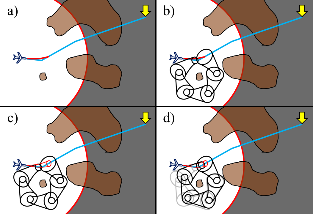
In this paper, we present a real-time trajectory planning algorithm that is both robust to bounded uncertainties and recursively feasible at the same time, without any need of braking capability. We begin by following the common planning framework, planning a global path to the goal through the free and unknown spaces, which is tracked by a receding horizon local trajectory in the free space. We guarantee recursive feasibility by attaching a loop of sequentially constructed funnels starting from the local trajectory. Robustness against uncertainties is guaranteed by requiring the forward reachable set (FRS) of the local trajectory to end inside the funnel loop. Suggested in [6], funnels are basically FRSs that start from a big initial set. If the system is located inside a funnel’s initial set, it can be provably driven to its exit by its associated controller. The set of pre-computed funnels, funnel library, can be used as building blocks for safe trajectory. If a funnel’s entrance encompasses another funnel’s exit, than the two funnels are sequentially composed and act like a single funnel. Fig. 1 briefly shows how the proposed planner runs. At an epoch, the planner finds the global and local trajectories, the FRS of the local trajectory, and a funnel loop that follows the local trajectory. A funnel loop acts like a single funnel whose entrance encompasses its exit, so the system can permanently stay inside the loop without braking.

We start by considering a nonlinear discrete-time time-invariant mobile robot system with state $x\in\mathbb{R}^{n}$ and input $u\in\mathbb{U}\subseteq\mathbb{R}^{m}$ under additive disturbance $w\in\mathbb{W}\subseteq\mathbb{R}^{n}$. The evolution of the system at any epoch $t$ is governed by

The state space consists of two components: cyclic and noncyclic coordinates. Let $x=(x_{\mathrm{c}},x_{\mathrm{nc}})\in\mathbb{R}^{n}$, where $x_{\mathrm{c}}\in\mathbb{R}^{d}$ and $x_{\mathrm{nc}}\in\mathbb{R}^{n-d}$ are the cyclic and noncyclic parts, respectively. The system’s governing equation is assumed to be invariant under translation in the cyclic coordinates, i.e., we can write

where $\hat{f}\mathrel{\mathop{\mathchar 58\relax}}\mathbb{R}^{n-d}\times\mathbb{R}^{m}\rightarrow\mathbb{R}^{n}$ is a function only of noncyclic coordinates and input. In mobile robot systems, the cyclic coordinates are usually their position in the Euclidean workspace. The cyclic component can be obtained using the projection map $\Pi\mathrel{\mathop{\mathchar 58\relax}}\mathbb{R}^{n}\rightarrow\mathbb{R}^{d}$:

The remaining parts of this paper assume that the cyclic coordinates of the system is equal to the robot’s position, hence collision checking can be done by just examining the cyclic coordinates.

A funnel $\mathcal{F}=(I,E,X)$ is a tuple consisting of three sets: entrance $I\subseteq\mathbb{R}^{n}$ and exit $X\subseteq\mathbb{R}^{n}$ in the state space, encompassing shape $E\subseteq\mathbb{R}^{d}$ in the Euclidean workspace. Mathematically, if $x(t_{0})\in I$, then there exists an epoch $t_{1}>t_{0}$ and $u(t,x(t),\cdots)\in\mathbb{U}\;\;,\forall t\in[t_{0},t_{1}]$, such that $x(t_{1})\in X$ and $\Pi(x(t))\in E,\;\;\forall t\in[t_{0},t_{1}]$. In this paper, we consider funnels that satisfy the following:

• •

  The entrance $I$ is of the form $I=\{(p,x_{\mathrm{nc}})\in\mathbb{R}^{n}\;|\;p\in\Pi(I),x_{\mathrm{nc}}\in I_{\mathrm{nc}}\subseteq\mathbb{R}^{n-d}\}$, where $\Pi(I)=\{p\in\mathbb{R}^{d}\;|\;A_{I}(p-p_{I})\leq b_{I}\}$. $A_{I}$ and $b_{I}$ are matrix and column vector with appropriate sizes, respectively. That is, the constraints for cyclic and noncyclic coordinates are decoupled, and the cyclic coordinate part is a polytope. $p_{I}\in\mathbb{R}^{d}$ is the center of $I$, which is the starting point of the nominal trajectory that traverses the funnel.

• •

  The exit $X$ is of the form $X=\{(p,x_{\mathrm{nc}})\in\mathbb{X}\;|\;\mathinner{\!\left\lVert p-p_{X}\right\rVert}_{2}\leq r_{X},x_{\mathrm{nc}}\in X_{\mathrm{nc}}\subseteq\mathbb{R}^{n-d}\}$, where $p_{X}$ is the (cyclic) coordinate of the funnel exit, $r_{X}>0$ is the exit radius on the cyclic coordinate.

• •

  The encompassing shape $E$ is a polytope, i.e., $E=\{p\in\mathbb{R}^{d}\;|\;A_{E}p\leq b_{E}\}$, where $A_{E}$ is a matrix and $b_{E}$ is a column vector, both with appropriate sizes.

Additionally, for the sake of simple description, we normalize each row of $A_{I}$ and $A_{E}$ to be a unit vector.

We say that two funnels $\mathcal{F}_{i}=(I_{i},X_{i},E_{i})$ and $\mathcal{F}_{j}=(I_{j},X_{j},E_{j})$ are sequentially composed if the entrance of $\mathcal{F}_{j}$ completely encompasses $X_{i}$, i.e.,

so that starting in $I_{i}$ guarantees the existence of a trajectory that leads to $X_{j}$. We denote this using the $\rhd$ symbol, i.e., $\mathcal{F}_{i}\rhd\mathcal{F}_{j}$. If $\mathcal{F}_{1}\rhd\cdots\rhd\mathcal{F}_{n_{F}}$ and $\mathcal{F}_{n_{F}}\rhd\mathcal{F}_{1}$, the funnels form a loop, which the system can persistently stay within.

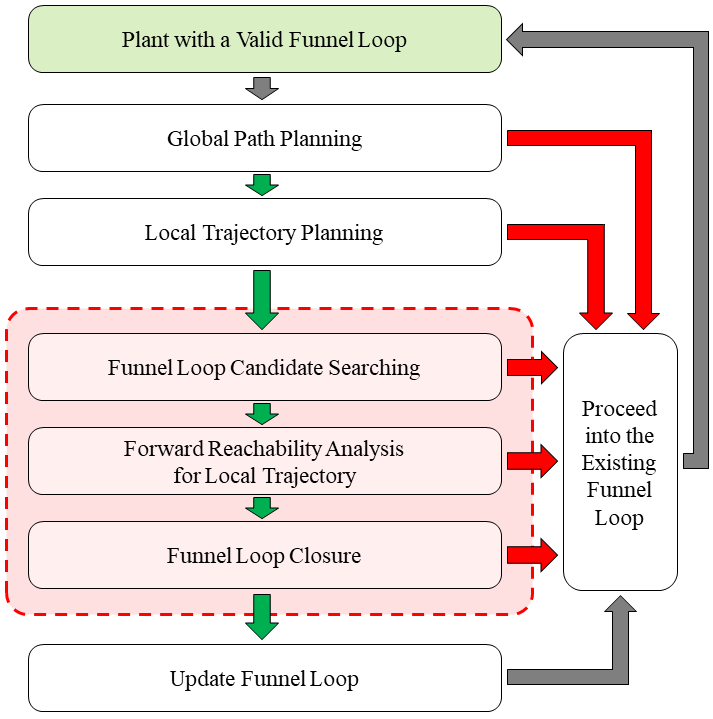
Our algorithm adds the following three steps to the global-local trajectory planning algorithm mentioned in the introduction: funnel loop candidate searching, forward reachability analysis, and funnel loop closure. In the funnel loop candidate searching step, we find a sequence of funnels which are expected to be adjustable in the cyclic coordinates to form a valid loop. The forward reachability analysis ensures that the planned local trajectory robustly drives the system into the entrance of the first funnel, despite the effect of disturbances. In the last step, the funnel positions are adjusted so that the loop is closed while maintaining collision avoidance and robustness of the local planner. As a result, we always have a funnel loop trajectory, which consists of a collision-free funnel loop and a robust local trajectory that drives the system into the loop. The system can stay inside the funnel loop as long as needed, before it finds a next valid funnel loop trajectory.

A schematic explanation of this procedure is given in Fig. 2. The proposed three steps are marked using a red box. Fig. 3 provides a graphical explanation of the algorithm. In the next section, we elucidate each step of the proposed algorithm.

For an ordered set of $n_{F}$ funnels $(\mathcal{F}_{1}=(I_{1},X_{1},E_{1})$, $\cdots$, $\mathcal{F}_{n_{F}}=(I_{n_{F}},X_{n_{F}},E_{n_{F}}))$ to form a valid loop, (4) should hold for all neighboring index pairs $(i,j)\in\mathbb{I}=\{(1,2),\cdots,(n_{F}-1,n_{F}),(n_{F},1)\}$. That is, to elaborate,

and

The goal of this section is to find $n_{F}$ funnels, each of them being a translated funnel from the funnel library $\mathfrak{F}=\{\mathcal{F}_{L\cdot 1},\cdots,\mathcal{F}_{L\cdot n_{\mathfrak{F}}}\}$, such that the funnels satisfy (5) and (6). We tackle this through a three-step process: in step 1, we find the funnel sequence that satisfies (5) completely and (6) roughly using a graph search algorithm (section IV-A); in step 2, we confirm that the local trajectory robustly leads to the entrance of the funnel trajectory candidate of step 1 (section IV-B); and in the last step, we adjust the positions of the funnel path candidate to completely satisfy (6) (section IV-C). This is possible owing to the funnel property that the constraints in the cyclic and noncyclic coordinates are decoupled.

To validate the proposed planning algorithm, an experiment was conducted using a ground rover shown in Fig. 6. The rover is an Ackerman steering robot equipped with an onboard computer (Intel NUC), a planar LiDAR sensor (YDLIDAR X4), and an IMU. The onboard computer has a 6-core CPU with base clock frequency of 1.10 GHz and 16 GB memory. The LiDAR scans the environment at 10 Hz. The planning algorithm is implemented in C++, and OSQP [23] is used for solving QPs. For real-time mapping and localization, Cartographer [24] is used. To provide a good initial guess to the SLAM module, pose estimates from the OptiTrack motion capture system and Intel Realsense Tracking Camera T265 are used. The map is updated every second.

The kinematics of the ground rover system is governed by the following bicycle-model equation:

where $x(t)=[p_{x}(t);p_{y}(t);\theta(t)]\in\mathbb{R}^{3}$, $u(t)=[v(t);\kappa(t)]\in\mathbb{R}^{2}$, and $w(t)=[w_{1}(t);w_{2}(t);w_{3}(t)]\in\mathbb{R}^{3}$ are the state, input, and disturbance vectors, respectively. The time discretization step $\delta t$ is a positive constant. The cyclic and noncyclic coordinates are $x_{\mathrm{c}}(t)=[p_{x}(t);p_{y}(t)]\in\mathbb{R}^{2}$ and $x_{\mathrm{nc}}(t)=[\theta(t)]\in\mathbb{R}^{1}$, respectively. We use the feedback controller in the following form to find the set point in speed $v_{s}(t)$ and turning rate $\kappa_{s}(t)$:

where $K_{p}$ and $K_{d}$ are gain matrices in appropriate sizes, $\Delta f$ and $\Delta l$ represent the forward and leftward displacements of the robot measured from the reference trajectory, respectively. $\Delta\theta$ is the deviation of the heading angle $\theta$ with respect to the reference. The function $\mathrm{sat}\mathrel{\mathop{\mathchar 58\relax}}\mathbb{R}^{2}\rightarrow\mathbb{R}^{2}$ clips the magnitude of the control commands to $\underline{u}\leq u(t)\leq\overline{u}$. The set points are forwarded to the low-level controller, which converts the set points to motor commands. The actual values of the parameters are summarized in Table  I.

To make the experiment more challenging, we restrict the speed of the reference trajectory to be fixed at 0.5 $\mathrm{m/s}$, and the turning rate (curvature) is limited to be less than 1.1 $\mathrm{m}^{-1}$. We however allow small jumps in the reference trajectory, and the tracking error due to jumps or external force is considered disturbance. The funnels and disturbance bound used in the experiment are obtained through a preliminary experiment, in which the tracking error is measured while successively running randomly chosen nominal trajectories. Fig. 7 shows the first five funnels used in the experiment, projected onto the cyclic coordinates. For the global planner, jump point search (JPS) [25] is used. The local planner is sampling-based: we keep a trajectory library consisting of 7 local trajectories and select on that best tracks the global trajectory. The A^⋆ algorithm is employed for the funnel loop candidate searching step, as it was one of the fastest among competing algorithms when used in the authors’ implementation.

The experiment consists of three scenarios. In each scenario, the robot runs in different environments, which are shown in Fig. 8. The goal positions change over time, and are given manually. In the experiment, the robot avoids the obstacle despite large tracking error, whose positions are a priori unknown, while keeping its (tracking) reference speed at 0.5 $\mathrm{m/s}$. The following subsections provide discussions about some important snippets taken from the experiment results.

In this paper, we presented a planning algorithm that can be run under disturbances in unknown environments, while guaranteeing safety without emergency brakes. We first start by planning global and local trajectories. A loop of sequentially composed funnels is constructed starting from the end of the local trajectory. Requiring the FRS of the local trajectory to lie within the funnel loop entrance guarantees that the system can be driven robustly into the funnel loop, in which it can stay permanently without collision, seeking for the chance of trajectory update. Experiment results showed that the planner can generate safe trajectories in real-time on onboard computers. It also demonstrated that the proposed algorithm is resilient to map changes, as the funnel loop is built locally.

Future work may include: enhancing the global planner so that it does not repeat planning through unreachable spaces; exploiting other symmetries in the funnel planning step, e.g., rotation; and extending this algorithm to multi-agent systems.

References

- [1] H. Seo, D. Lee, C. Y. Son, C. J. Tomlin, and H. J. Kim, “Robust trajectory planning for a multirotor against disturbance based on hamilton-jacobi reachability analysis,” in 2019 IEEE/RSJ International Conference on Intelligent Robots and Systems (IROS). IEEE, 2019, pp. 3150–3157.
- [2] S. L. Herbert, M. Chen, S. Han, S. Bansal, J. F. Fisac, and C. J. Tomlin, “Fastrack: A modular framework for fast and guaranteed safe motion planning,” in 2017 IEEE 56th Annual Conference on Decision and Control (CDC), 2017, pp. 1517–1522.
- [3] A. Majumdar and R. Tedrake, “Robust online motion planning with regions of finite time invariance,” in Algorithmic foundations of robotics X. Springer, 2013, pp. 543–558.
- [4] A. Liniger and J. Lygeros, “A viability approach for fast recursive feasible finite horizon path planning of autonomous rc cars,” in Proceedings of the 18th International Conference on Hybrid Systems: Computation and Control, 2015, pp. 1–10.
- [5] D. Fridovich-Keil, J. F. Fisac, and C. J. Tomlin, “Safely probabilistically complete real-time planning and exploration in unknown environments,” in 2019 International Conference on Robotics and Automation (ICRA). IEEE, 2019, pp. 7470–7476.
- [6] A. Majumdar and R. Tedrake, “Funnel libraries for real-time robust feedback motion planning,” The International Journal of Robotics Research, vol. 36, no. 8, pp. 947–982, 2017.
- [7] J. Tordesillas, B. T. Lopez, and J. P. How, “Faster: Fast and safe trajectory planner for flights in unknown environments,” in 2019 IEEE/RSJ international conference on intelligent robots and systems (IROS). IEEE, 2019, pp. 1934–1940.
- [8] S. Kousik, S. Vaskov, F. Bu, M. Johnson-Roberson, and R. Vasudevan, “Bridging the gap between safety and real-time performance in receding-horizon trajectory design for mobile robots,” The International Journal of Robotics Research, vol. 39, no. 12, pp. 1419–1469, 2020.
- [9] S. Bansal, M. Chen, S. Herbert, and C. J. Tomlin, “Hamilton-jacobi reachability: A brief overview and recent advances,” in 2017 IEEE 56th Annual Conference on Decision and Control (CDC). IEEE, 2017, pp. 2242–2253.
- [10] J. Ding, E. Li, H. Huang, and C. J. Tomlin, “Reachability-based synthesis of feedback policies for motion planning under bounded disturbances,” in 2011 IEEE International Conference on Robotics and Automation. IEEE, 2011, pp. 2160–2165.
- [11] H. Seo, C. Y. Son, and H. J. Kim, “Fast funnel computation using multivariate bernstein polynomial,” IEEE Robotics and Automation Letters, pp. 1–1, 2021.
- [12] S. Singh, A. Majumdar, J.-J. Slotine, and M. Pavone, “Robust online motion planning via contraction theory and convex optimization,” in 2017 IEEE International Conference on Robotics and Automation (ICRA). IEEE, 2017, pp. 5883–5890.
- [13] M. E. Villanueva, B. Houska, and B. Chachuat, “Unified framework for the propagation of continuous-time enclosures for parametric nonlinear odes,” Journal of Global Optimization, vol. 62, no. 3, pp. 575–613, 2015.
- [14] M. E. Villanueva, R. Quirynen, M. Diehl, B. Chachuat, and B. Houska, “Robust mpc via min–max differential inequalities,” Automatica, vol. 77, pp. 311–321, 2017.
- [15] H. Seo, C. Y. Son, D. Lee, and H. J. Kim, “Trajectory planning with safety guaranty for a multirotor based on the forward and backward reachability analysis,” in 2020 IEEE International Conference on Robotics and Automation (ICRA). IEEE, 2020, pp. 7142–7148.
- [16] T. Fraichard and H. Asama, “Inevitable collision states—a step towards safer robots?” Advanced Robotics, vol. 18, no. 10, pp. 1001–1024, 2004.
- [17] H. Oleynikova, Z. Taylor, R. Siegwart, and J. Nieto, “Safe local exploration for replanning in cluttered unknown environments for microaerial vehicles,” IEEE Robotics and Automation Letters, vol. 3, no. 3, pp. 1474–1481, 2018.
- [18] T. Schouwenaars, J. How, and E. Feron, “Decentralized cooperative trajectory planning of multiple aircraft with hard safety guarantees,” in AIAA Guidance, Navigation, and Control Conference and Exhibit, 2004, p. 5141.
- [19] B. Eysenbach, S. Gu, J. Ibarz, and S. Levine, “Leave no trace: Learning to reset for safe and autonomous reinforcement learning,” arXiv preprint arXiv:1711.06782, 2017.
- [20] I. Jang, D. Lee, and H. J. Kim, “Provably safe real-time receding horizon trajectory planning for linear time-invariant systems,” in 2020 20th International Conference on Control, Automation and Systems (ICCAS). IEEE, 2020, pp. 612–616.
- [21] S. Liu, M. Watterson, K. Mohta, K. Sun, S. Bhattacharya, C. J. Taylor, and V. Kumar, “Planning dynamically feasible trajectories for quadrotors using safe flight corridors in 3-d complex environments,” IEEE Robotics and Automation Letters, vol. 2, no. 3, pp. 1688–1695, 2017.
- [22] R. Deits and R. Tedrake, “Computing large convex regions of obstacle-free space through semidefinite programming,” in Algorithmic foundations of robotics XI. Springer, 2015, pp. 109–124.
- [23] B. Stellato, G. Banjac, P. Goulart, A. Bemporad, and S. Boyd, “Osqp: An operator splitting solver for quadratic programs,” Mathematical Programming Computation, pp. 1–36, 2020.
- [24] W. Hess, D. Kohler, H. Rapp, and D. Andor, “Real-time loop closure in 2d lidar slam,” in 2016 IEEE International Conference on Robotics and Automation (ICRA). IEEE, 2016, pp. 1271–1278.
- [25] D. Harabor and A. Grastien, “Online graph pruning for pathfinding on grid maps,” in Proceedings of the AAAI Conference on Artificial Intelligence, vol. 25, no. 1, 2011.