Driven dissipative preparation of few-body Laughlin states of Rydberg polaritons in twisted cavities
Abstract
We present a driven dissipative protocol for creating an optical analog of the Laughlin state in a system of Rydberg polaritons in a twisted optical cavity. We envision resonantly driving the system into a 4-polariton state by injecting photons in carefully selected modes. The dissipative nature of the polariton-polariton interactions leads to a decay into a two-polariton analog of the Laughlin state. Generalizations of this technique could be used to explore fractional statistics and anyon based quantum information processing. We also model recent experiments that attempt to coherently drive into this same state.
I Introduction
Efforts to produce analogs of fractional quantum Hall effects Stormer et al. 1999 in atomic Bloch et al. 2008; Bloch et al. 2012; Wilkin and Gunn 2000; Paredes et al. 2003; Wilkin and Gunn 2000; Paredes et al. 2001; Cooper 2008; Barberán et al. 2006; Cooper et al. 2001; Sørensen et al. 2005; Hafezi et al. 2007; Zhang et al. 2016; Cooper and Dalibard 2013; Roncaglia et al. 2011; Gemelke et al. 2010 and optical settings Ozawa et al. 2019; Maghrebi et al. 2015a; Anderson et al. 2016; Hafezi et al. 2013; Chang et al. 2008; Birnbaum et al. 2005; Wu et al. 2017; Schine et al. 2016 are driven by the desire to directly observe and manipulate “anyon” excitations, which act as particles with unconventional quantum statistics Arovas et al. 1984; Stern 2008; Camino et al. 2005; Muñoz de las Heras et al. 2020. In addition to being of fundamental interest, these anyons can be useful for quantum information processing Kitaev 2003; Georgiev 2017; Kapit et al. 2012; Kapit et al. 2014. Here we give a driven dissipative protocol for producing a minimal quantum Hall state in a system of Rydberg polaritons in a non-coplaner optical cavity.
The quantum Hall effect is seen in 2D electron systems in large magnetic fields. As argued by Schine et al. Schine et al. 2016, there is a one-to-one correspondence between quantum state of such electrons and the optical modes of a non-coplanar (or twisted) cavity. This correspondence has lead to a number of proposals to use twisted cavities to reproduce quantum Hall physics Maghrebi et al. 2015a; Dutta and Mueller 2018. In order to produce an analog of electron-electron interactions, these proposals hybridize the photon modes in the cavity with long-lived Rydberg excitations of an atomic gas. The resulting Rydberg polaritons interact via a strong dipole-dipole interaction, which can be modelled as a short-range repulsion Béguin et al. 2013. At particular filling factors, the ground state is expected to be a fractional quantum Hall state.
A key difference between the electronic and optical system is that polariton number is not conserved: One readily injects polaritons into the cavity by shining an appropriately tuned laser on the system; Polaritons decay due to the finite cavity lifetime, or in inelastic scattering processes. Here we take advantage of this feature, and show that one can drive this system in such a way that it naturally evolves into an analog of the Laughlin state, one of the most iconic examples of fractional quantum Hall states Laughlin 1983.
Our scheme is in the spirit of other driven-dissipative state preparation protocols Diehl et al. 2008; Kraus et al. 2008; Verstraete et al. 2009; Diehl et al. 2011; Cian et al. 2019; Sharma and Mueller 2021; Budich et al. 2015; Bardyn et al. 2013; Reiter et al. 2016; Umucal ılar and Carusotto 2012, which have analogs in autonomous error correction Albert et al. 2019; Freeman et al. 2017; Gertler et al. 2021; Combes 2021; Liu et al. 2016; Cohen and Mirrahimi 2014; Gau et al. 2020a; Gau et al. 2020b. The basic idea is that you want to construct a situation where the state of interest is a “dark state” which is neither excited by the drive, nor decays through the dissipative channel. We rely upon one of the key features of the Laughlin state, namely that it vanishes when two electrons come close together. In the Rydberg polariton context, this means that inelastic two-body loss is strongly suppressed in the Laughlin state. We construct a drive which takes the system to an excited state, which then decays into the Laughlin state.
In section II we present our model of Rydberg Polaritons in twisted cavities. We analyze the dynamics via a Lindblad equation, and in section III we describe our numerical approach. In section IV we validate our model by reproducing the observations from Clark et al. 2020, including calculating the pair correlations functions of emitted photons, one of the key signatures used in the experiment. Section V uses our validated model to introduce our driven dissipative protocol for producing the Laughlin state and provides our numerical study of the dynamics. Section VI briefly describes how one can verify that that our approach is successful.
II Modeling
Researchers in Chicago have designed an optical cavity where the modes are in one-to-one correspondence to the quantum states of 2D harmonically trapped charged particle in a magnetic field.
An atomic gas is placed in the cavity, and the cavity modes hybridize with a long-lived Rydberg excitation. An idealized effective model Dutta and Mueller 2018 for the resulting polaritons, in the cavity’s image plane, is with
| (1) |
The operator annihilates a polariton at location , defined in the 2D plane. The effective vector potential corresponds to a uniform effective magnetic field, and is related to the non-coplanarity of the cavity. We use the symmetric gauge and take . The coefficients and are related to the cavity geometry and the amount of mixing between the photon modes and the Rydberg excitation. The polariton-polariton interaction comes from the dipole-dipole interaction between the Rydberg excitations. It is short-ranged, and as long as the cavity is sufficiently large it can be replaced by a local potential . Some technical details of arriving at this description are given in Appendix A.
The modes which diagonalize Eq. (II) have frequencies , where , and which is half the cyclotron frequency Fock 1928; Darwin 1927. When (or equivalently ), modes with different have the same energy. These nearly-degenerate modes make up the lowest Landau level, and have wavefunctions,
| (2) |
with normalization,
| (3) |
The characteristic length is .
When multiple polaritons are in the cavity, the interaction term, Eq. (1), breaks this degeneracy. The preeminent role of the interactions leads to highly non-trivial physics. The ground state of this model when there is one polariton for every two modes is the Laughlin state Laughlin 1983; Clark et al. 2020. It boasts fractionally charged anyonic excitations. When there is one polariton per mode, and the interactions are appropriate, one instead finds the Pfaffian, with non-abelian excitations Regnault and Jolicoeur 2003. The goal of these experiments is to produce such states and demonstrate their exotic properties.
The defining feature of the state is that it is the highest density state which vanishes whenever two polaritons touch:
| (4) |
As a first step, Clark et al. have isolated three of the modes from Eq. (2), corresponding to (all with ). This is sufficient to produce a 2-polariton analog of the Laughlin state,
| (5) |
Given the three accessible modes, this is the state with the largest number of polaritons that vanishes when two polaritons touch. It can also be written as
| (6) |
where and .
Our goal is to construct a protocol for producing the two-photon state, . Once this goal is achieved, one can consider generalizations that will lead to the many-body state in Eq. (4).
We project into the relevant space, writing
| (7) |
where and are given by Eqs. (2) and (3). This equation defines the annihilation operators . In order to model the experiment, we restrict the sum to be over – but in a future experiment it could run over the entire lowest Landau level.
| (8) |
where the coefficient vanishes unless , in which case it is
| (9) |
Although we do not make use of it, this interaction is separable: . One can readily verify that Eq. (6) is in the null-space of .
Polaritons can be injected into the cavity by shining lasers with appropriately shaped wavefronts onto the cavity mirror. This can be modelled by
| (10) |
Here is the frequency of the laser which couples to mode . As long as one can remove all time dependence by shifting to a rotating frame, in which case the single-particle Hamiltonian is with
| (11) | ||||
here is the detuning of the drive from mode .

Polaritons are lost through several processes, which we model using a Lindblad rate equation for the density matrix ,
| (12) |
Both the cavity modes and the the Rydberg excitations have finite lifetimes. These are modelled by the jump operators .
They contribute
| (13) |
where
| (14) |
We treat the single-photon loss rate as independent of the mode index, .
We also model collisional losses. As argued in Appendix A, one can engineer the system so that the dominant collisional loss channel involves a process where two proximate polaritons are simultaneously lost. This is described by
| (15) | |||||
| (16) |
Crucially, the decay rate is proportional to the interaction energy, and states with zero interaction energy are infinitely long-lived. This means that in the absence of single particle loss the Laughlin state has an infinite lifetime. When restricted to three modes (), the only long-lived states will be the vacuum, the single-polariton states, and the two-photon Laughlin state in Eq. (6). All others decay due to these two-polariton processes
We will use these incoherent processes as resources to produce the Laughlin state by engineering a drive which will excite the system to the four-polariton manifold, relying on loss to populate the long-lived Laughlin state.
Figure 1 shows the energy eigenvalues of , with or fewer polaritons. The vertical axis corresponds to energy, and the horizontal axis to angular momentum . As depicted by the three arrows extending from the vacuum state, the -drive couples states which are vertically separated, while the and drives cause diagonal transitions. The thickness of each energy level corresponds to the decay rate from the collisional two-polariton loss.
In this diagram, sets of lines have labels which correspond to the angular momenta of the polaritons in the state. For example, the states above the label 3,9 and 6,6 are the Laughlin state , and the state . As denoted by dashed horizontal lines, in the absence of interactions, all states with polaritons, would have energy , where is the bare cavity frequency. The collisional decay rate is proportional to the interaction energy, so the linewidth grows as one moves away from the dashed line.
III Numerical Techniques
We use two different numerical techniques to analyze the Lindblad equation. First, we numerically integrate Eq. (12), using a Runge Kutta finite difference scheme. This gives us the full time evolution of the density matrix . In our full model, .
Alternatively, we vectorize the Lindblad equation interpreting as a length vector, . The Lindblad equation becomes , with
| (17) |
The steady state corresponds to the kernel of the matrix . We numerically find the nullspace of using standard linear algebra libraries.
IV Validation
Before implementing our dissipative approach to generating the Laughlin state, we validate parts of our model by reproducing the experimental observations in
Clark et al. 2020. In addition to giving us the opportunity to compare to experimental results, the simpler nature of this experiment lets us explicitly write down all expressions, making our arguments more concrete.
In Clark et al. 2020 the experimentalists resonantly drive the mode: . The other two modes are undriven: . Since the states ,, and are resonantly coupled, and the drive strengths are low, there is essentially zero probability to end up in any other state except these three, and the states they decay into: and . It therefore suffices to truncate to the simplified model depicted in Fig. 2.

In the rotating frame, the Hamiltonian is
| (18) |
where the basis states are . The matrix elements are
| (19) | ||||
| (20) |

None of these states experience collisional losses, so we only need to consider the single-photon loss terms, corresponding to jump operators
| (21) | ||||
| (22) | ||||
| (23) |
We numerically integrate the Lindblad equation,
| (24) |
Starting from the vacuum state at time . Figure 3 shows typical results for the time evolution of the probablility of being in the Laughlin state .
If the drive is weak compared to the single-photon loss rate, , then very few polaritons are ever in the cavity: As soon as a polariton is created, it decays. In the opposite limit , damped Rabi oscillations are seen. As shown in the inset, the steady-state population of the two-photon Laughlin state is a monotonic function of the drive amplitude, saturating at roughly 21 when the drive is very strong.

In the experiment Clark et al. 2020, , and one therefore expects that the steady-state ensemble only has a 1.8 probability of being in the Laughlin state. To verify that they have produced the Laughlin state, the experimentalists use a correlation measurement: If two photons are simultaneously emitted from the cavity, then the cavity must have been in a two-polariton state.
Aspects of the two-photon state can be extracted from the mode-structure of the outcoming photons. This can be thought of as a form of post-selecting: “What is the quantum state when two polaritons are in the cavity?”
More precisely, the experimentalists measure the steady state correlation function , where is the joint probability of measuring a photon in mode at time and another in mode at time . This quantity is normalized by the the product of the probabilities of measuring each of these events separately, and . In steady-state the denominator is time independent.
Results from our numerical calculations are shown in Fig. 4. In the top panel one sees that sequential photons in the 6-mode are anticorrelated. At delay ,
| (25) |
where and are the steady state probabilities of being in the or states. The rate of emitting a photon from is , while the rate for emitting from is .
For large delay, , as the two events are uncorrelated. The photons are anticorrelated at short times because once a photon is emitted from the state, a second cannot be emitted until another photon enters the cavity.
For larger one sees weak oscillations in the correlation function, as Rabi oscillations between the states make certain delays less likely than others.
The photons in the and modes are positively correlated. Whenever a photon is emitted, a photon must follow at a later time. At zero time delay
| (26) | |||||
where, as before, the rate of emission from to is : and . Equation (26) can be somewhat simplified by using the principle of balance: , and . This yields
| (27) |
When is small, then the time between emission of the individual photons in a 3-9 pair is short compared to the time between event pairs. This leads to a large correlation peak. At long times , as one is detecting photons from different pairs. The correlation function should just fall exponentially between these values, with decay time .
To numerically calculate , we first integrate Eq. (24) for a long time to produce the steady state density matrix . We calculate the emission rates . The density matrix immediately following a -photon emission event is . We then evolve this density matrix for time to calculate , and .
Another important probe in Clark et al. 2020 is to compare the probability of simultaneously observing a and photon, to that of finding two photons,
| (28) |
Within this truncated model, the only contributions to the correlation functions come from the diagonal element of corresponding to the Laughlin state,
| (29) | |||||
| (30) |
The experimental results are within error bars of this number, which is consistent with producing the Laughlin state.
V Driven-Dissipative Preparation of the 2-polariton Laughlin State

As illustrated by the model in Sec. IV, in the absence of careful timing, one cannot efficiently produce the Laughlin state by resonant coupling. This is a generic feature of coherent quantum systems: For example, resonantly coupling the levels of a two-level system will not create a steady-state inverted population. On the other hand, a laser can be made from a 3-level atom. There one produces a large occupation of an excited metastable state by driving to a third level which decays into it. We will explore the many-body analog of this approach. Four-polariton states play the analog of the unstable excited level, and the Laughlin state plays the role of the metastable excited level. Collisional two-polariton loss provides the decay from the four-polariton manifold to the Laughlin state.
The challenge in designing this protocol is that many levels are involved. Figure 1 shows a complicated network of 35 levels. Each polariton states couple to three states with N+1 polaritons. This gives 60 distinct transition matrix elements. One needs to be able to efficiently couple the vacuum state to the four-photon manifold without coupling the Laughlin state to any other level. Moreover there are a large number of parameters, including the amplitude and frequencies of the three drives, the interaction strength, and the various decay constants.
The challenge would be greatly reduced if we had a technique to coherently inject 4-photons, directly coupling the vacuum state to the four-polariton manifold. Appendix B analyzes that simplified case. Here we tackle the full problem, where the drive is of the form in Eq. (11).
Exciting the system into the 4-polariton manifold is a fourth order process – which will be very strongly suppressed when the drive is weak. One cannot simply increase the drive strength, as a strong drive will also deplete the Laughlin state. Our strategy for overcoming this difficulty is to engineer a string of intermediate states. Ideally the photons would be absorbed through four resonant (or near resonant) transitions. Simultaneously we need the Laughlin state to be spectrally isolated.
We adjust the detunings , , and to optimize this process. As previously explained, in order to have a well-defined rotating frame, we require . Furthermore, we require that the four-photon transition is resonant. There are ten 4-polariton states which have a finite probability to decay into the Laughlin state. As a concrete example, consider , with interaction energy . To resonantly couple to this state, we need . Throughout we use units where and take . We neglect single-polariton loss, taking .
Figure 5 illustrates the role of resonances by plotting the steady-state probability of being in the Laughlin state as a function of , calculated by the technique in Sec. III. Here we fix , so that the state remains degenerate with the vacuum state, in the rotating frame. One sees at least six discrete peaks, corresponding to when various intermediate states become resonant. The most prominent peaks correspond to the simultaneous alignment of multiple intermediate states. Figure 6 shows energy level diagrams corresponding to the three largest peaks. These depict the rotating-frame energy of the states from Fig. 1, separated into columns, each of which represents a different number of polaritons. As illustrated by the arrows, the drive changes the polariton number by 1, and hence connects states in neighboring columns. Two-polariton collisional loss causes an incoherent decay into a state which is two columns to the left. Energy conservation is relevant to the coherent drive processes, but not the loss processes. As before, the line-widths are shown by the thickness of the lines. These three energy level diagrams illustrate the central design principles behind our approach.
The most important feature of the level diagrams in Fig. 6 is the fact that there is a direct chain of near-resonant excitations that takes one to the four-polariton manifold. The closer these intermediate states are to resonance, the higher the effective transition rate to the four-polariton state. The second most important feature is how spectrally isolated the Laughlin state is. The reason that the peak marked (*) is higher than the one marked (***) is that the Laughlin state is more isolated. One is led to the intuitive recipe: Align the the levels needed to absorb photons, but keep the Laughlin state isolated.
The second highest (**) peak in Fig. 5 is qualitatively different than the others, as the Laughlin state is coherently coupled to the vacuum. In that sense it is more similar to the scenario in Sec. IV, and it shares the qualitative features of that model. There are however two differences. First, in this section we are driving with , , and , while in Sec. IV only was nonzero. The three drives add coherently, and result in a somewhat larger population of the Laughlin state. The other difference between this scenario and Sec. IV is that there are 3-polariton and 4-polariton states which are also resonant. The minimal model here requires including these two additional states, resulting in a 7 dimensional Hilbert space.
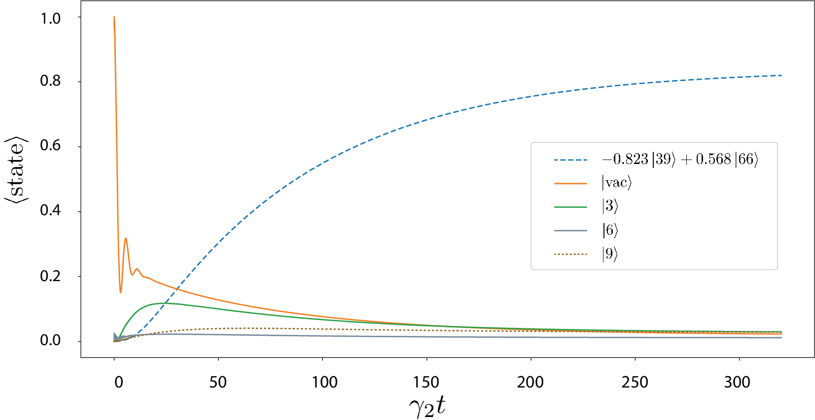
As shown in Fig. 7, the probability of ending up in the Laughlin state is a non-monotonic function of the drive-strength. For weak drive, the bottle-neck is populating the four-photon manifold. In this regime, the population of the Laughlin state increases with drive strength. The rate of increase depends on the accuracy of the alignment of the intermediate states: Thus for small the solid red curve (corresponding to the peak with a single asterisk in Fig. 5) rises slower than the dotted green curve (corresponding to three asterisks). As should be apparent, the physics of the dashed curve is somewhat different, as the Laughlin state is resonantly excited.
If the drive is made too strong, the probability of ending up in the Laughlin state falls. This occurs because the drive excites the system out of the Laughlin state.
The story is somewhat complicated by the fact that there are three different ’s. Figure 8 further explores the amplitude dependence of the (*) peak in Fig. 5. We set and vary and . The most prominent feature is a peak at , and a ridge which extends out from it at an angle. This ridge is a quantum interference effect: For a certain ratio of , the excitations to the four-polariton manifold are enhanced. Due to the presence of many different intermediate states, and many states which couple to the Laughlin state, the structure can be quite rich: For example, the dotted green curve in Fig. 7 has a dip near , and the red curve has several kink-like features.

We systematically explored all ten potential four-photon transitions, producing the analog of Fig. 5 for each of them. For each of the large peaks we numerically optimized the values of and . The most favorable example is the one in Fig. 6 which resulted in a steady-state occupation of the Laughlin state of 83.9% with , and .
VI Measurements
The most easily interpreted probe of our system is monitoring the light emitted by the two-polariton loss events. No such events occur in the Laughlin state, and the disappearance of this signal is a direct measurement of the short range polariton-polariton correlation function. Analogous correlation measurements were carried out in atomic systems Gemelke et al. 2010. The challenge of this measurement is that the light is presumably emitted in random directions. Furthermore, this signal cannot distinguish between different dark states.
A slightly more indirect, but simpler measurement is monitoring the reflected light from the drive. Any photons which enter the cavity show up as an attenuation of this reflected light. Thus when the system reaches the Laughlin state, which is dark, the reflected intensity increases. Again, any dark state would give the same signal.
A third approach is to monitor the intensity and correlations of the light emitted through single-polariton losses, as was discussed in Sec. IV. Since this probe is harder to interpret, it is not as useful as a “smoking gun.” Its primary advantage is that the measurement is relatively straightforward.
VII Summary and Discussion
We presented a driven dissipative approach to producing the two-particle Laughlin state of polaritons in a twisted cavity. This is part of a broader goal of producing and braiding anyons in an AMO system.
Producing the two-particle Laughlin state is a modest, but necessary step towards this goal. Our technique is a useful complement to existing proposals, and it brings with it a number of pros and cons.
Most importantly, our technique is self-correcting: If a perturbation (such as decay of a polariton) knocks the system out of the Laughlin state, the driven-dissipative process will bring you back. It also does not rely upon any careful timing.
Unfortunately, our technique does require fine-tuning the of the drive frequencies and amplitudes. In an experiment, this fine-tuning would need to be done by trial and error, as our models have finite accuracy. These experiments also require a hierarchy of energies which may be difficult to attain – namely: . Here is the rate of single-photon loss, is the drive strength, is the rate of interaction-driven two-photon loss, and is the interaction strength. The most challenging aspect, requiring novel cavities, is making smaller than the other scales. The relative size of and can be controlled by adjusting the detuning of the EIT transition used for the Rydberg polaritons (Appendix A). The drive strengths are under direct experimental control.
A crucial question is the scalability of the approach. The biggest impediment here is that as one adds more states, the energy-level spectrum becomes quite dense. Consequently even more fine-tuning would be needed to create larger Laughlin states. Nonetheless, this driven-dissipative approach is a valuable tool for state creation and stabilization.
VIII Acknowledgements
We thank Jon Simon and his group for fruitful discussions. This work was supported by NSF PHY-1806357.
Appendix A Microscopic Model of interacting Rydberg Polaritons in nearly degenerate multimode cavity
For completeness we give a brief derivation of the model from Sec. II. We make no attempt at mathematical rigor – more thorough treatments can be found elsewhere Georgakopoulos et al. 2018; Bienias et al. 2014; Gullans et al. 2016; Gorshkov et al. 2011; Maghrebi et al. 2015b.
The modes of an optical cavity are labeled by a longitudinal index , and transverse indices . In the image plane, where the atoms sit, the electric field has magnitude . We are considering the case where several modes with the same are nearly degenerate. We consider only those modes, and drop the longitudinal index in our expressions. For simplicity we will assume that the form a complete set of states in the plane. If they do not, we can always formally add the missing states, giving them an infinite energy.
The operator which creates a photon in mode is , and can define an operator which creates a maximally focussed beam as
| (31) |
By the completeness property, these obey the standard Bose commutation relations. The Hamiltonian can be expressed as
| (32) | |||||
| (33) |
which defines the kernel .
At every point in space we envision a large number of 3-level atoms, with ground state , a short lived excited state , and a long-lived excited Rydberg state . The cavity photons couple the states and , and a control beam couples and . We introduce operators and that change the number of excitations at , and work in a rotating frame. The Hamiltonian describing these degrees of freedom are
| (34) |
Here , where is the detuning of the p-state from resonance and is the lifetime of that state. Here and are the energies of the states in the lab frame, and is the frequency of the control laser. The Rabi frequencies from the cavity and control lasers are and . Since this Hamiltonian is strictly local, we have left off the position arguments in the operators.
It is convenient to transform to a basis which diagonalizes Eq. (34),
| (35) | |||||
| (36) | |||||
| (37) |
These represent the long-lived dark polaritons, with energy and the short-lived bright polaritons with energies
| (38) |
The relationships in Eq. (35) through (37) can be inverted to write
| (39) |
where . We substitute this into Eq. (33). There are nine terms, but the bright polaritons are far off resonance. Keeping only the terms involving the dark polaritons,
| (40) |
where
| (41) |
and is the difference between the Rydberg excitation energy and the control frequency. It appears due to transforming into the rotating frame. It simply shifts the entire spectrum, and has no physical consequences.
Our truncation is only valid if the spectrum of is small compared to the splitting between polaritons . The influence of the discarded modes can be treated perturbatively Georgakopoulos et al. 2018.
The Rydberg atoms interact via a dipole-dipole interaction,
| (42) |
where the interaction is typically modeled as – though the exact potential is more complicated Weber et al. 2017. The challenge here is that can be much larger than any of the other scales, and hence mixes in the other polariton modes. It is large, however, only in a small region of space. Thus its effect on the modes is captured by a zero-range potential
| (43) |
The coefficient is found by matching the low-energy scattering phase shifts, for example by summing a set of ladder diagrams Bienias et al. 2014. Due to mixing in the dark polariton states, these interactions generically contain an inelastic piece. As we argue below, when is small, both of the polaritons in the collision are lost. In a Lindblad formalism, this corresponds to the jump operator in Eq. (15).
While the full analysis of the scattering problem is tedious, the central physics is apparent by considering two polaritons at fixed locations, and . The Hilbert space is then 9-dimensional, as all three flavors of polaritons will be mixed. We are considering the case where is small, so the state with two dark polaritons is nearly degenerate with the state containing one of each flavor of bright polaritons . When is small compared to , we can truncate to these two states. In the basis , the local Hamiltonian is then
| (44) |
with
| (45) | |||||
| (46) | |||||
| (47) |
If the state is an eigenstate, with energy 0. For non-zero interactions the state continuously connected with that one has an admixture of and its energy is found by solving a quadratic equation. For , the mixing is weak, and the potential that the polariton feels is just the Rydberg-Rydberg coupling scaled by the overlap with the Rydberg state
| (48) |
When the interaction is strong, , the eigenstate is independent of and the effective interaction is proportional to ,
| (49) |
Within this framework, the fact that this energy is complex indicates there is particle loss. Since the loss comes from coupling to the state with two bright polaritons, two particles are lost.
As argued in Georgakopoulos et al. 2018, when is sufficiently large, one will also have collisional loss events where only one of the polaritons are lost. These will dominate if . Thus for our driven-dissipative state preparation scheme to work, we require that we are in the regime where is small.
Appendix B Multi-photon drive
Our protocol faces two challenges: (1) efficiently exciting from the vacuum state to the metastable 4-polariton manifold, and (2) avoiding driving the system out of the Laughlin state. Both of these difficulties would be avoided if we could directly inject 4 photons into the system, for example with a drive term of the form
| (50) |
Under those circumstances the Laughlin state is a true dark state (in the absence of single-particle loss). In this Appendix we briefly explore the dynamics under this hypothetical drive, contrasting it with a two-photon drive
| (51) |
and the single-photon drive used in the main text. In this latter case, we take .
As in the main text, we use units where , and take , but we use a significantly stronger 2-body decay rate . The latter sets the characteristic scale for the incoherent transitions from the four-polariton manifold to the Laughlin state, and the widths of various resonances.
There are three different four-polariton states which can be excited by these drives. They are resonant when = 0.31, 0.19, 0.12. Figure 10 shows the probability of being in the Laughlin state after a time , for different drive strengths. We choose to look at the finite-time probabilities, as in our 4-photon drive model the Laughlin state is a true dark state, and if one waits long enough the system will have a 100% chance of occupying that state.
The top panel of Fig. 10 shows results for the four-photon drive. The dominant feature is a large peak near . This corresponds to the transition with the largest coupling matrix element. Smaller peaks are visible near the other resonances. As the drive amplitude increase, the maximum probability saturates at 100%, and spreads into a plateau.
The two-photon drive (middle panel) shows the same three peaks, with an additional feature closer to . This corresponds to a two-photon resonance. Generically the probabilities of occupying the Laughlin state are smaller for the two-photon drive than for the four-photon drive. Note that interactions in the intermediate two-polariton states mix the different polariton flavors, enhancing the compared to what is seen in the top figure.
The single-photon drive (bottom panel) shows essentially zero occupation of the Laughlin state, unless the drive is very strong. This is because with only the drive there is no way to arrange a set of resonant intermediate states. The location of the peak that appears near for very strong drive is a compromise between the final-state and intermediate-state resonances.

References
- Stormer et al. (1999) H. L. Stormer, D. C. Tsui, and A. C. Gossard, Rev. Mod. Phys. 71, S298 (1999).
- Bloch et al. (2008) I. Bloch, J. Dalibard, and W. Zwerger, Rev. Mod. Phys. 80, 885 (2008).
- Bloch et al. (2012) I. Bloch, J. Dalibard, and S. Nascimbène, Nature Physics 8, 267 (2012).
- Wilkin and Gunn (2000) N. Wilkin and J. Gunn, Physical Review Letters 84, 6 (2000).
- Paredes et al. (2003) B. Paredes, P. Zoller, and J. Cirac, Solid State Communications 127, 155 (2003).
- Paredes et al. (2001) B. Paredes, P. Fedichev, J. I. Cirac, and P. Zoller, Phys. Rev. Lett. 87, 010402 (2001).
- Cooper (2008) N. Cooper, Advances in Physics 57, 539 (2008) .
- Barberán et al. (2006) N. Barberán, M. Lewenstein, K. Osterloh, and D. Dagnino, Phys. Rev. A 73, 063623 (2006).
- Cooper et al. (2001) N. R. Cooper, N. K. Wilkin, and J. M. F. Gunn, Phys. Rev. Lett. 87, 120405 (2001).
- Sørensen et al. (2005) A. S. Sørensen, E. Demler, and M. D. Lukin, Phys. Rev. Lett. 94, 086803 (2005).
- Hafezi et al. (2007) M. Hafezi, A. S. Sørensen, E. Demler, and M. D. Lukin, Phys. Rev. A 76, 023613 (2007).
- Zhang et al. (2016) J. Zhang, J. Beugnon, and S. Nascimbene, Phys. Rev. A 94, 043610 (2016).
- Cooper and Dalibard (2013) N. R. Cooper and J. Dalibard, Phys. Rev. Lett. 110, 185301 (2013).
- Roncaglia et al. (2011) M. Roncaglia, M. Rizzi, and J. Dalibard, Sci Rep 1 (2011) .
- Gemelke et al. (2010) N. Gemelke, E. Sarajlic, and S. Chu, “Rotating few-body atomic systems in the fractional quantum hall regime,” (2010), arXiv:1007.2677 [cond-mat.quant-gas] .
- Ozawa et al. (2019) T. Ozawa, H. M. Price, A. Amo, N. Goldman, M. Hafezi, L. Lu, M. C. Rechtsman, D. Schuster, J. Simon, O. Zilberberg, , and I. Carusotto, Rev. Mod. Phys. 91, 015006 (2019).
- Maghrebi et al. (2015a) M. F. Maghrebi, N. Y. Yao, M. Hafezi, T. Pohl, O. Firstenberg, and A. V. Gorshkov, Physical Review A 91, 033838 (2015a).
- Anderson et al. (2016) B. M. Anderson, R. Ma, C. Owens, D. I. Schuster, and J. Simon, Phys. Rev. X 6, 041043 (2016).
- Hafezi et al. (2013) M. Hafezi, M. D. Lukin, and J. M. Taylor, New Journal of Physics 15, 063001 (2013).
- Chang et al. (2008) D. E. Chang, V. Gritsev, G. Morigi, V. Vuletic, M. D. Lukin, and E. A. Demler, Nature Physics 4, 884 (2008).
- Birnbaum et al. (2005) K. M. Birnbaum, A. Boca, R. Miller, A. D. Boozer, T. E. Northup, and H. J. Kimble, Nature 436, 87 (2005).
- Wu et al. (2017) Y.-H. Wu, H.-H. Tu, and G. J. Sreejith, Phys. Rev. A 96, 033622 (2017).
- Schine et al. (2016) N. Schine, A. Ryou, A. Gromov, A. Sommer, and J. Simon, Nature 534, 671 (2016).
- Arovas et al. (1984) D. Arovas, J. R. Schrieffer, and F. Wilczek, Phys. Rev. Lett. 53, 722 (1984).
- Stern (2008) A. Stern, Annals of Physics 323, 204 (2008), january Special Issue 2008.
- Camino et al. (2005) F. E. Camino, W. Zhou, and V. J. Goldman, Phys. Rev. B 72, 075342 (2005).
- Muñoz de las Heras et al. (2020) A. Muñoz de las Heras, E. Macaluso, and I. Carusotto, Phys. Rev. X 10, 041058 (2020).
- Kitaev (2003) A. Kitaev, Annals of Physics 303, 2 (2003).
- Georgiev (2017) L. S. Georgiev, in Quantum Systems in Physics, Chemistry, and Biology, edited by A. Tadjer, R. Pavlov, J. Maruani, E. J. Brändas, and G. Delgado-Barrio (Springer International Publishing, Cham, 2017) pp. 75–94.
- Kapit et al. (2012) E. Kapit, P. Ginsparg, and E. Mueller, Phys. Rev. Lett. 108, 066802 (2012).
- Kapit et al. (2014) E. Kapit, M. Hafezi, and S. H. Simon, Phys. Rev. X 4, 031039 (2014).
- Dutta and Mueller (2018) S. Dutta and E. J. Mueller, Phys. Rev. A 97, 033825 (2018).
- Béguin et al. (2013) L. Baguin, A. Vernier, R. Chicireanu, T. Lahaye, and A. Browaeys, Phys. Rev. Lett. 110, 263201 (2013).
- Laughlin (1983) R. B. Laughlin, Phys. Rev. Lett. 50, 1395 (1983).
- Diehl et al. (2008) S. Diehl, A. Micheli, A. Kantian, B. Kraus, H. P. Büchler, and P. Zoller, Nature Physics 4, 878 (2008).
- Kraus et al. (2008) B. Kraus, H. P. Büchler, S. Diehl, A. Kantian, A. Micheli, and P. Zoller, Phys. Rev. A 78, 042307 (2008).
- Verstraete et al. (2009) F. Verstraete, M. M. Wolf, and I. J. Cirac, Nature Physics 5, 633 (2009).
- Diehl et al. (2011) S. Diehl, E. Rico, M. A. Baranov, and P. Zoller, Nature Physics 7, 971 (2011).
- Cian et al. (2019) Z.-P. Cian, G. Zhu, S.-K. Chu, A. Seif, W. DeGottardi, L. Jiang, and M. Hafezi, Phys. Rev. Lett. 123, 063602 (2019).
- Sharma and Mueller (2021) V. Sharma and E. J. Mueller, “Driven-dissipative control of cold atoms in tilted optical lattices,” (2021), arXiv:2101.00547 [cond-mat.quant-gas] .
- Budich et al. (2015) J. C. Budich, P. Zoller, and S. Diehl, Phys. Rev. A 91, 042117 (2015).
- Bardyn et al. (2013) C.-E. Bardyn, M. A. Baranov, C. V. Kraus, E. Rico, A. İmamoğlu, P. Zoller, and S. Diehl, New Journal of Physics 15, 085001 (2013).
- Reiter et al. (2016) F. Reiter, D. Reeb, and A. S. Sørensen, Phys. Rev. Lett. 117, 040501 (2016).
- Umucal ılar and Carusotto (2012) R. O. Umucal ılar and I. Carusotto, Phys. Rev. Lett. 108, 206809 (2012).
- Albert et al. (2019) V. V. Albert, S. O. Mundhada, A. Grimm, S. Touzard, M. H. Devoret, and L. Jiang, Quantum Science and Technology 4, 035007 (2019).
- Freeman et al. (2017) C. D. Freeman, C. M. Herdman, and K. B. Whaley, Phys. Rev. A 96, 012311 (2017).
- Gertler et al. (2021) J. M. Gertler, B. Baker, J. Li, S. Shirol, J. Koch, and C. Wang, Nature 590, 243 (2021).
- Combes (2021) J. Combes, Nature Physics 17, 437 (2021), .
- Liu et al. (2016) Y. Liu, S. Shankar, N. Ofek, M. Hatridge, A. Narla, K. M. Sliwa, L. Frunzio, R. J. Schoelkopf, and M. H. Devoret, Phys. Rev. X 6, 011022 (2016).
- Cohen and Mirrahimi (2014) J. Cohen and M. Mirrahimi, Phys. Rev. A 90, 062344 (2014).
- Gau et al. (2020a) M. Gau, R. Egger, A. Zazunov, and Y. Gefen, Phys. Rev. B 102, 134501 (2020a).
- Gau et al. (2020b) M. Gau, R. Egger, A. Zazunov, and Y. Gefen, Phys. Rev. Lett. 125, 147701 (2020b).
- Clark et al. (2020) L. W. Clark, N. Schine, C. Baum, J. Ningyuan, and J. Simon, Nature 582 (2020), .
- Fock (1928) V. Fock, Zeitschrift für Physik 47, 446 (1928).
- Darwin (1927) C. G. Darwin, Proc. Royal Soc. London 117, 258 (1927).
- Regnault and Jolicoeur (2003) N. Regnault and T. Jolicoeur, Phys. Rev. Lett. 91, 030402 (2003).
- Georgakopoulos et al. (2018) A. Georgakopoulos, A. Sommer, and J. Simon, Quantum Science and Technology 4, 014005 (2018).
- Bienias et al. (2014) P. Bienias, S. Choi, O. Firstenberg, M. F. Maghrebi, M. Gullans, M. D. Lukin, A. V. Gorshkov, and H. P. Büchler, Phys. Rev. A 90, 053804 (2014).
- Gullans et al. (2016) M. J. Gullans, J. D. Thompson, Y. Wang, Q.-Y. Liang, V. Vuletić, M. D. Lukin, and A. V. Gorshkov, Phys. Rev. Lett. 117, 113601 (2016).
- Gorshkov et al. (2011) A. V. Gorshkov, J. Otterbach, M. Fleischhauer, T. Pohl, and M. D. Lukin, Phys. Rev. Lett. 107, 133602 (2011).
- Maghrebi et al. (2015b) M. F. Maghrebi, M. J. Gullans, P. Bienias, S. Choi, I. Martin, O. Firstenberg, M. D. Lukin, H. P. Büchler, and A. V. Gorshkov, Phys. Rev. Lett. 115, 123601 (2015b).
- Weber et al. (2017) S. Weber, C. Tresp, H. Menke, A. Urvoy, O. Firstenberg, H. P. Büchler, and S. Hofferberth, Journal of Physics B: Atomic, Molecular and Optical Physics 50, 133001 (2017).