The volume of the black hole interior at late times

Among the greatest challenges in physics is obtaining a microscopic understanding of the expanding universe. While this is presently out of reach for the observed universe, an intriguing example of such an expanding spacetime is the interior of black holes, which in turn can be studied in the framework of the AdS/CFT correspondence Maldacena:1997re; Witten:1998qj; Gubser:1998bc. It has been proposed by Susskind and collaborators that the growth of the black hole interior is dual to the growth of complexity, the minimal number of gates required for a quantum circuit to prepare the corresponding time evolved state in the dual CFT Susskind:2014rva; Susskind:2014moa. One version of this proposal is that complexity equals the volume of a maximal slice in the black hole interior Stanford:2014jda.¹¹ 1 Both the definition of complexity and the size of the black hole interior suffer from many ambiguities, which have lead to many versions of this proposal Brown:2015bva; Brown:2015lvg; Couch:2016exn; Belin:2021. However, these ambiguities are believed not to affect the late time universal scaling properties. The most important rationale behind this conjecture is that the black hole interior grows for a very long time, past when conventional probes, like correlation functions or entanglement entropy, have already reached their thermal equilibrium value. Complexity, on the other hand, is expected to grow in chaotic systems at the same rate as the volume of the interior, until times exponentially large in the entropy, after which it saturates in a complexity plateau Susskind:2015toa; Brown:2016wib; Balasubramanian:2019wgd; Susskind:2020wwe; Balasubramanian:2021mxo; Haferkamp:2021uxo. Up to this point, it has been an open problem to establish whether the volume of the black hole interior exhibits a similar saturation at late times.

A priori, there is no reason to expect that a geometrical description of the interior could capture the late time saturation of complexity. However, recent developments show that the gravitational path integral has a surprisingly large regime of validity, with the exponentially small corrections coming from summing over topologies being capable of capturing fine details of spectral statistics Saad:2019lba; Cotler:2020ugk; Belin:2020hea, or the unitary Page curve of the entropy of an evaporating black hole Almheiri:2019qdq; Penington:2019kki. Emboldened by this success, in this paper, we calculate the corrections coming from higher topologies to the volume of the black hole interior in a wide class of models of two-dimensional gravity, including the widely studied theory of JT gravity Teitelboim:1983ux; Jackiw:1984je; Maldacena:2016upp. Importantly, this requires us to give a nonperturbative definition of the length of the black hole interior and to complete the sum over surfaces of higher topology to the matrix model of Saad-Shenker-Stanford Saad:2019lba (or its generalizations Witten:2020wvy; Maxfield:2020ale). We indeed find that the length of the black hole interior saturates at a time and length exponentially large in the entropy. Our result thus provides a non-perturbative version of the complexity equals volume conjecture.

In section 2 we propose a natural candidate for the length $\langle\ell\rangle$ of the Einstein-Rosen (ER) bridge. In a two-dimensional theory, the volume of the black hole interior is given by length of the geodesic going from one side to the other. While the definition of this length is unambiguous on surfaces with trivial topology, on manifolds of higher genus there are an infinite number of geodesic spanning between the two sides of the ER bridge. We explore various definitions for this length and settle on one that is well defined on surfaces of arbitrary topology, causes minimal backreaction on the metric, and can be analytically continued between Euclidean and Lorentzian geometries:

where ${{\gamma}}$ is labeling non self-intersecting geodesics, $\langle\dots\rangle$ evaluates the gravitational path integral by summing over surfaces with any topology and where ${{\Delta}}$ acts as a regulator. Since the free field boundary-to-boundary propagator on hyperbolic surfaces is given by the sum over geodesics (including self-intersecting ones), $\langle\ell\rangle$ is closely related to the two-point function $\langle\chi\chi\rangle$, with an operator of dimension ${{\Delta}}$ inserted on each side of the two-sided black hole, as a probe for the black hole interior.

In section 3, we turn to the analysis of this quantity. In the limit in which $\chi$ is a probe field and when we approximate the two-point function by summing over non self-intersecting geodesics, we prove that at arbitrary order in $e^{S_{0}}$ (with $S_{0}$ being the leading order entropy of the black hole) the two-point function is simply given by

where ${{\mathcal{M}}}_{{\Delta}}(E_{1},E_{2})=\absolutevalue{\<E_1|\chi|E_2\>}^{2}$ can be computed analytically. This result can be viewed as a generalization to arbitrary genus and dilaton potential of the genus 1 result for JT gravity of Saad:2019lba. The expression (1.2) is also consistent with a conjectured formula for the matter two-point function in gravity that was obtained by studying operator insertions in the matrix integral that is dual to the JT theory Saad:2019lba; Blommaert:2020seb.

In section 4 we obtain the main result of our paper, that is, up to an overall additive constant²² 2 The linear growth of the black hole interior at time scales $t\ll e^{S_{0}}$ but exactly in the temperature was first obtained in Yang:2018gdb.

in a large class of theories of dilaton gravity, including JT gravity. Here, the coefficients $C_{1}$ is $O(1)$ while $C_{0}$ is $O\left(e^{S_{0}}\right)$ and depend on the spectral density $\rho(E)$ in each dilaton gravity model and on the inverse-temperature $\beta$ of the thermofield double state in which the system is prepared at $t=0$. For a plot of $\langle\ell(t)\rangle$ see figure 1.

In section 5 we remark on the late-time differences between the ER bridge length, the spectral form factor, and the two-point function. While all three quantities exhibit a period of growth and then a plateau at later times, the physics of the growth and plateau periods for the bridge is widely different from that for the latter two quantities. While the period of growth for the ER bridge length is due to the contribution from the classical solution, the “ramp” in the spectral form factor and two-point function is due to the leading Euclidean wormhole geometry. More importantly, while the “plateau” in the spectral form factor and two-point function occurs due to a cancellation between the wormhole geometry and other non-perturbative corrections to the spectral two-point function $\left\langle\rho(E_{1})\rho(E_{2})\right\rangle$, the saturation of the bridge length is due to novel cancellations between the classical disconnected contribution and non-perturbative contributions in $\left\langle\rho(E_{1})\rho(E_{2})\right\rangle$. To our knowledge, these types of cancellations have not been noticed in the random matrix literature before and are universal in all one matrix models.

To further probe the relation between complexity and the late time length of the ER bridge, we compute the variance of the latter quantity in section 6. We start by deriving a geometric formula for the variance in terms of the spectral four-point function. We then show that at late times

In contrast to the plateaus for the spectral form factor and the two-point function, on the plateau for the ER bridge, the “signal” is much larger than the “noise” in the regime $t\ll e^{2S_{0}}$. However, we find that as opposed to $\langle\ell\rangle$, the variance $\sigma_{\ell}$ does not have a plateau, instead it grows forever, in particular, it becomes the same order as the signal when $t\propto e^{2S_{0}}$. We will discuss some possible explanations for this unexpected behavior.

Finally, in section 7 we discuss the interpretation of our results beyond the theories of dilaton gravity and their matrix integral dual. Our geometric computation suggests the importance of a new spectral quantity, called spectral complexity, which we expect to closely track the volume of the black interior in any chaotic system with a holographic dual. We confirm this expectation in a numerical study of the SYK model.

We want to define the length $\expectationvalue{\ell}$ of the ER bridge in two-dimensional models of gravity. Our definition needs to take into account that in higher genus geometries, there are multiple geodesics connecting two boundary points. Furthermore, when we probe this length we do not wish to experience strong back-reaction from the measurement since that might spoil the growth of the ER bridge.

One is first tempted to consider the minimal length geodesic spanning between the two sides of the ER bridge as the definition of $\ell$. However, in a gravitational path integral, we oftentimes have to work with complexified geometries and complex geodesic lengths. Consequently, the minimum geodesic length cannot be analytically continued. Alternatively, one might imagine computing the minimal length of the ER bridge by considering the two-sided two point function $\langle\chi_{L}(t)\chi_{R}(0)\rangle$ and taking the limit $-\lim_{\Delta\to\infty}\frac{1}{\Delta}\log\langle\chi_{L}(t)\chi_{R}(0)\rangle=\lim_{\Delta\to\infty}\frac{1}{\Delta}\langle\sum_{{{\gamma}}}\,e^{-{{\Delta}}\ell_{{\gamma}}}\rangle$ which seemingly picks the geodesic with minimal real part from the sum.³³ 3 Here, $L/R$ denotes operators inserted on the left/right sides of the bridge. However, due to the backreaction of the operator insertion on the metric the measurement of the ER bridge length is spoiled: as shown in Yang:2018gdb for any $\Delta>0$, the two-point function decays exponentially up to a time $t\sim O(1)$, past which it transitions to a power law decay due to quantum corrections coming from JT gravity ($\sim 1/t^{3}$, regardless of the value of $\Delta$). Because of this, $-\lim_{\Delta\to\infty}\frac{1}{\Delta}\log\langle\chi_{L}(t)\chi_{R}(0)\rangle$ does not see the growth of the ER bridge past the thermalization time (which is $\sim\beta$). Therefore, we dismiss these candidates when defining the length of the bridge.

A candidate that resolves all the issues above is the regularized sum⁴⁴ 4 We will specify the exact meaning of $\langle\dots\rangle$ shortly.

where ${{\gamma}}$ is labeling non self-intersecting geodesics and $\langle\dots\rangle$ evaluates the sum over geodesics within the JT gravity or dilaton gravity path integral, including the contribution of surfaces of arbitrary genus. The prescription for choosing geodesics without self-intersections is natural since, if we cut the manifold open along such curves, we obtain a state in which the boundary points are separated by geodesic length $\ell_{{\gamma}}$.⁵⁵ 5 The cut that separates the manifold into two disjoint parts will in general also create some accompanying baby universes. From the quantum information perspective, this choice makes contact with the original motivation of interpreting $\expectationvalue{\ell}$ as a length of a minimal tensor network that can create the state. Furthermore, this quantity can be analytically continued and has minimal backreaction on the metric.⁶⁶ 6 We can think about this quantity as inserting a tensionful defect and extracting the leading correction in the tensionless limit. This is similar to how the minimal surface is obtained from the gravitational Rényi entropies using the replica trick Lewkowycz:2013nqa. However, one might worry that (2.1) could be divergent since it involves an infinite number of geodesics on all surfaces with $g>1$. As we show shortly, we find that the time-dependent piece in (2.1) is finite, independent of the regularization scheme, and is precisely the probe of the late time physics that we are interested in: i.e., it is sufficient to study $\langle\ell(t)\rangle-\langle\ell(0)\rangle$.

We will compute $\langle\ell(t)\rangle$ by taking the ${{\Delta}}$ derivative of the two-sided correlation function, computed in an approximation, where we drop self-intersecting geodesics. Explicitly,

Two-sided correlation functions can be obtained by analytic continuation from Euclidean correlators, and it will be convenient to obtain $\left\langle\chi_{L}\left(t\right)\chi_{R}\left(0\right)\right\rangle$ from a Euclidean computation performed in section 3. The analytic continuation that we use is valid in any quantum system

where in the first line we used the two-sided (thermofield double) and in the second the Euclidean representation. The last expression in the first line is the most intuitively connected to the ER bridge length where we evolved both the left and rightt boundary points forward in time equally by $t/2$.⁷⁷ 7 Recall that in the thermofield double in the right system the natural time direction runs backwards. The equality between the first and second lines can be established by inserting a complete set of states in the second line and using that the thermofield double state is $\ket{\text{TFD}_\beta}=\sum_{n}e^{-\beta R_{n}/2}\ket{E_n}_{L}\ket{E_n^*}_{R}$. The dilaton gravity theories considered in this paper are famously ensembles of quantum systems, random matrix theories, so when we apply (2.3) in our context, the gravity computation gives the ensemble average of the above quantities.

In section 3, we will shown that $\left\langle\chi(x_{1})\chi(x_{2})\right\rangle_{\text{non-int.}}$ is a particularly nice quantity in JT gravity and other theories of dilaton gravity, as it can be computed to all orders in the genus expansion and can even be computed non-perturbatively using the matrix model representation for such gravitational theories. We will therefore use (2.2) to extract $\langle\ell(t)\rangle-\langle\ell(0)\rangle$.

JT gravity is a theory of two-dimensional gravity with a metric $g_{\mu\nu}$, coupled to a dilaton $\phi$, whose Euclidean action is given by Teitelboim:1983ux; Jackiw:1984je; Maldacena:2016upp

The first term is purely topological, as it only accounts for the Euler characteristic of the manifold ${\mathcal{M}}$. The bulk term fixes the geometry to be a patch of hyperbolic space whose boundary has fixed, large, proper length $L=\beta/\epsilon$ and dilaton value $\phi=1/\epsilon$.⁸⁸ 8 Since we set the boundary value of the dilaton to one, times and inverse temperatures in the rest of the paper are measured in these units. In particular the Schwarzian theory is strongly coupled when $\beta\gg 1$. These boundary conditions require the presence of the Gibbons-Hawking-York term, which gives an action for the boundary fluctuations in each such hyperbolic patch. While the model exhibits great simplicity since it only depends on topological data and boundary fluctuations, it still has black hole solutions and, in particular, we will be interested in studying two-sided black holes, which have an ER bridge between the two sides.

In this section, our goal is to probe the length of the ER bridge when one includes the contribution of surfaces with arbitrary topology to the gravitational path integral in (3.1). The probe that we shall consider is the boundary-to-boundary two-point function of a probe matter field $\chi$, with scaling dimension $\Delta$, which only couples to the metric in the JT theory. In the probe limit, the two-point function on any hyperbolic surface can be schematically expressed as

where the sum over ${\mathcal{M}}$ is a sum over all surfaces, obeying the boundary conditions discussed above, and the sum over $\gamma$ is a sum over all geodesics connecting the points at boundary times $x_{1}$ and $x_{2}$, each of length $\ell_{\gamma}$.

To clarify our notation for expectation values of observables in the gravitational path integral, $\Tr_{\beta}(\dots)\equiv\Tr(e^{-\beta H} \dots)$ is a mnemonic for the insertion of a gravitational boundary with the boundary conditions described above while the $\dots$ will indicate what operators are inserted on each boundary. Finally, the $\langle\dots\rangle$ will represent the evaluation of the gravitational path integral with a number of boundaries given by the number of traces inside, each with its own specified operator insertions.

On a hyperbolic surface of genus $g\geq 1$, there will be an infinite number of geodesics $\gamma$, some of which will self-intersect. Since we are interested in the two-point function in order to probe the length $\ell_{\gamma}$ of the ER bridge in a two-sided black hole, we shall restrict ourselves to geodesics that do not self-intersect and set $x_{1}=0$ and $x_{2}=\frac{\beta}{2}+it$; for each surface ${\mathcal{M}}$ we will denote such geodesics going from $x_{1}$ to $x_{2}$ by $\mathcal{G}_{x_{1},x_{2}}$ and will denote correlators that solely account for these geodesics by $\langle\dots\rangle_{\text{non-int.}}$.⁹⁹ 9 Since we discarded self-intersecting geodesics, $\langle\Tr_{\beta}\left(\chi(x_{1})\chi(x_{2})\right)\rangle_{\text{non-int.}}$ is only an approximation to the full two-point function. It was argued by Saad Saad:2019pqd that this approximation gives the leading behavior of the function for large Lorentzian times, and he computed this modified two-point function to the first subleading order in $e^{S_{0}}$ given by the genus 1 geometry. The leading disk contribution (which does not suffer from this ambiguity) was obtained in Mertens:2017mtv. Since in this paper, our focus is on studying the length of the ER bridge and not on the full two-point function, we will not further discuss whether self-intersecting geodesics are important in its late-time behavior.

In JT gravity, the path integral over all metrics reduces to an integral over boundary wiggles which we denote by $D{(\mathcal{W})}$ and an integral over the moduli space of hyperbolic surfaces Saad:2019lba. Therefore, the two-point function can be rewritten as

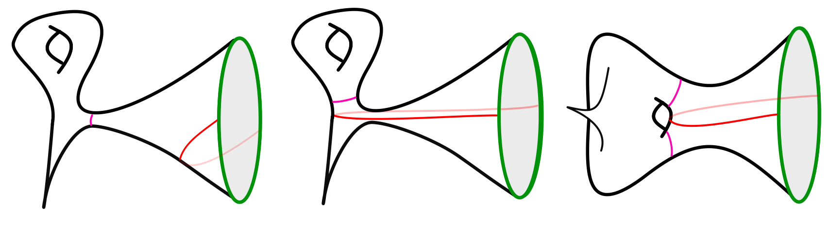
where $\omega=\sum_{j=1}^{3g-3+n}db\wedge d\tau$ is the Weil-Peterson symplectic form on the moduli space of hyperbolic surfaces, and $\mathcal{T}_{g,1}$ represents the moduli space of all hyperbolic surfaces ${\mathcal{M}}_{g,1}$ of genus $g$ with $1$ asymptotic boundary. Due to the redundancy of large diffeomorphism in the gravitational path integral, we are supposed to quotient this moduli space by the mapping class group $\text{Mod}({\mathcal{M}}_{g,1})$ of ${\mathcal{M}}_{g,1}$. As in the example shown in figure 2, cutting along each geodesic $\gamma$ in the sum above, we can either obtain two disconnected manifolds, each with a single boundary, ${\mathcal{M}}_{h,1}$ and ${\mathcal{M}}_{g-h,1}$ with $0\leq h\leq g$, or a single connected manifold with two boundaries ${\mathcal{M}}_{g-1,\,2}$. The mapping class group acts by relating all boundary-to-boundary geodesics within a given cutting class as well as all closed geodesics on ${\mathcal{M}}_{h,1}$ and ${\mathcal{M}}_{g-h,1}$ (or ${\mathcal{M}}_{g-1,\,2}$ in the latter case) which do not intersect the boundary-to-boundary geodesic. Therefore, following a similar strategy as in mirzakhani2007simple; Saad:2019pqd; Blommaert:2020seb, we can rewrite the integral over the moduli space as

where $\ell$ is the length of a geodesic which is now part of the boundary of ${\mathcal{M}}_{h,1}$ and ${\mathcal{M}}_{g-h,1}$ (or part of both boundaries of ${\mathcal{M}}_{g-1,2}$) and where for the remainder of the paper the sum over $h$ is bounded such that disconnected surfaces of genus $h$ and $g-h$ are not counted twice. When the genus $g=2$, we can use figure 2 to better understand (3.4). The first term on the RHS sums over the moduli space of the genus one surface with two boundaries obtained after cutting the rightmost figure along the red geodesic. The $h=0$ term in (3.4) corresponds to the sum over the moduli space of the leftmost figure after a cut along the red geodesic which results into a one boundary genus zero and a one boundary genus one surface, while the $h=1$ term correspond to summing over the moduli space of the two genus one surfaces obtained after the cut in the center figure.

As drawn in figure 2, we can now cut each such surface along the closed geodesic which is closest to the asymptotic boundary to separate the manifolds, into two bordered Riemann surfaces with a geodesic boundary (or a single such surface in the case of ${\mathcal{M}}_{g-1,2}$), and two trumpets which, on one end, have a closed geodesic boundary, and, on the other end, have a boundary with fixed proper length and fixed dilaton glued to a geodesic of fixed length, $\ell$. Following the wavefunctional formalism discussed in Yang:2018gdb, we denote the path integral for such an object as $\psi_{\text{Trumpet},x}(\ell,b)$. The expression for the trumpet wavefunction was derived in Saad:2019pqd in terms of the Hartle-Hawking wavefunction for a disk with a fixed ADM mass $E$, cut by a geodesic boundary of length $\ell$, $\psi_{\text{Disk, E}}(\ell)$:

$$\begin{split}\psi_{\text{Trumpet, }x}(\ell,b)=\hbox to116.66pt{\vbox to70.34pt{\pgfpicture\makeatletter\hbox{\hskip 62.66956pt\lower-35.82727pt\hbox to0.0pt{\lxSVG@begingroup@{_scopebegin} \lxSVG@begingroup@{stroke} \lxSVG@begingroup@{fill} \lxSVG@setlinewidth{\the\pgflinewidth}\lxSVG@begingroup@{stroke-width} \lx@inpgf@ignorespaces\nullfont\hbox to0.0pt{\lxSVG@begingroup@{_scopebegin} {{\lx@inpgf@ignorespaces}} {{{\lx@inpgf@ignorespaces}}{{\lx@inpgf@ignorespaces}}{{\lx@inpgf@ignorespaces}}{{}}{{}}{{}}{{}}\lxSVG@begingroup@{_scopebegin} \lxSVG@transformcm{0.6}{0.0}{0.0}{0.6}{0.0pt}{0.0pt}\lxSVG@begingroup@{transform} \pgfsys@hbox{55}\lxSVG@closescope }at (0,0); {}{{}}{}{{}}{}\lxSVG@stroke\lxSVG@drawpath@unclipped{M -79.13 0}{fill:none} \lx@inpgf@ignorespaces\hbox{\hbox{{\lxSVG@begingroup@{_scopebegin} {{}{}{{ {}{}}}{ {}{}} {{}{{\lx@inpgf@ignorespaces}}}{{}{\lx@inpgf@ignorespaces}}{}{{}{\lx@inpgf@ignorespaces}} {\lx@inpgf@ignorespaces }{{{{\lx@inpgf@ignorespaces}}\lxSVG@begingroup@{_scopebegin} \lxSVG@transformcm{1.0}{0.0}{0.0}{1.0}{-59.33655pt}{-3.47221pt}\lxSVG@begingroup@{transform} \pgfsys@hbox{58}\lxSVG@closescope }}} \lxSVG@closescope }}} {}{{}}{}{{}}{}\lxSVG@stroke\lxSVG@drawpath@unclipped{M 11.81 -40.16}{fill:none} \lx@inpgf@ignorespaces\hbox{\hbox{{\lxSVG@begingroup@{_scopebegin} {{}{}{{ {}{}}}{ {}{}} {{}{{\lx@inpgf@ignorespaces}}}{{}{\lx@inpgf@ignorespaces}}{}{{}{\lx@inpgf@ignorespaces}} {\lx@inpgf@ignorespaces }{{{{\lx@inpgf@ignorespaces}}\lxSVG@begingroup@{_scopebegin} \lxSVG@transformcm{1.0}{0.0}{0.0}{1.0}{6.45256pt}{-32.49426pt}\lxSVG@begingroup@{transform} \pgfsys@hbox{58}\lxSVG@closescope }}} \lxSVG@closescope }}} {}{{}}{}{{}}{}\lxSVG@stroke\lxSVG@drawpath@unclipped{M 66.14 40.16}{fill:none} \lx@inpgf@ignorespaces\hbox{\hbox{{\lxSVG@begingroup@{_scopebegin} {{}{}{{ {}{}}}{ {}{}} {{}{{\lx@inpgf@ignorespaces}}}{{}{\lx@inpgf@ignorespaces}}{}{{}{\lx@inpgf@ignorespaces}} {\lx@inpgf@ignorespaces }{{{{\lx@inpgf@ignorespaces}}\lxSVG@begingroup@{_scopebegin} \lxSVG@transformcm{1.0}{0.0}{0.0}{1.0}{44.94353pt}{26.86928pt}\lxSVG@begingroup@{transform} \pgfsys@hbox{58}\lxSVG@closescope }}} \lxSVG@closescope }}} \lxSVG@closescope {{ {}{}{}{\lx@inpgf@ignorespaces}{\lx@inpgf@ignorespaces}}{{{\lx@inpgf@ignorespaces}}{{}}}}{\lx@inpgf@ignorespaces}{\lx@inpgf@ignorespaces}\hss}\lxSVG@discardpath\lxSVG@closescope \hss}}\lxSVG@closescope\endpgfpicture}}=\int_{0}^{\infty}dE\rho_{\text{Trumpet}}(E)\psi_{\text{Disk},\,E}(\ell)e^{-xE}\,,\end{split}$$

(3.5)

where the density of states of the trumpet $\rho_{\text{Trumpet}}(E)=\frac{\cos(b\sqrt{2E})}{\pi\sqrt{2E}}$ can be computed from fermionic localization Stanford:2017thb, while $\psi_{\text{Disk},E}(\ell)$ is given by $\psi_{\text{Disk},E}(\ell)=4e^{-\ell/2}K_{i\sqrt{8E}}(e^{-\ell/2})$ Yang:2018gdb. Here, $E$ can be interpreted as the ADM mass observed on the asymptotic boundary and the conservation of this mass follows from the orthogonality relation

Above, $\rho_{\text{Disk}}(E)$ is the density of states in JT gravity on the disk, given by $\rho_{\text{Disk}}(E)=\sinh(2\pi\sqrt{E})$Stanford:2019vob. Using (3.4) we can thus rewrite the genus $g$ contribution,¹⁰¹⁰ 10 The integral over $\omega$ in (3.4) can thus be rewritten by separating the integral over the moduli of the two closed geodesics separating the trumpets from the bordered Riemann surfaces, $\int_{\frac{\mathcal{T}_{h,1}}{\text{Mod}({\mathcal{M}}_{h,1})}}\omega=\int_{0}^{\infty}db\int_{0}^{b}d\tau\int_{\frac{\tilde{\mathcal{T}}_{h,1}(b)}{\text{Mod}(\tilde{\mathcal{M}}_{h,1}(b))}}\omega$ $\bigg($and $\int_{\frac{\mathcal{T}_{g-1,2}}{\text{Mod}({\mathcal{M}}_{g-1,2})}}\omega=\int_{0}^{\infty}db_{1}\int_{0}^{b}d\tau_{1}\int_{0}^{\infty}db_{2}\int_{0}^{b}d\tau_{2}\int_{\frac{\tilde{\mathcal{T}}_{g-1,2}(b_{1},b_{2})}{\text{Mod}(\tilde{\mathcal{M}}_{g-1,2}(b_{1},b_{2}))}}\omega\bigg)$ where the $\tilde{\,}$ signifies that we are considering the moduli space of surfaces with one (or two) geodesic boundary of fixed length $b$ (or $b_{1}$ and $b_{2}$).

where, in order to compactly write (3.7), and not have to consider cuts which involve the disk wavefunction separately, we have formally chosen ${{\mathrm{Vol}}}_{0,1}(b)$ to be such that, after the integral over $b$, the disk wavefunction is recovered¹¹¹¹ 11 This is possible since ${{\mathrm{Vol}}}_{0,1}(b)$ (or its Laplace transform) does not enter the topological recursion used to determine ${{\mathrm{Vol}}}_{g,n}$.

This formula can be seen as a generalization of the result from Saad:2019lba which computed the boundary-to-boundary two-point function up to genus one, up to arbitrary genus. Inserting (3.5) into (3.7), using the orthogonality relation (3.6) and performing the integral over $\ell$ explicitly, we can more conveniently rewrite (3.7) as

where $\left\langle\rho(E_{1})\rho(E_{2})\right\rangle^{\text{JT}}$ is the spectral two-point function in JT gravity. The leading disk contribution of (3.9) has been derived using a variety of techniques Yang:2018gdb; Mertens:2017mtv; Blommaert:2018oro; Kitaev:2018wpr; Iliesiu:2019xuh, while the arbitrary genus generalization found in (3.9) was hinted at by studying two-point function insertions directly in the matrix integral dual to JT gravity Saad:2019pqd; Blommaert:2020seb. In these works ${{\mathcal{M}}}_{{\Delta}}(E_{1},E_{2})$ was identified with the squared matrix element $\absolutevalue{\chi}^{2}_{E_{1},E_{2}}=\absolutevalue{\<E_1|\chi|E_2\>}^{2}$, evaluated in the energy basis. The formula (3.9) can also be derived using a matrix model description of JT gravity coupled to a scalar field jafferismatrix.¹²¹² 12 We thank Daniel Jafferis for explaining this to us.

The spectral two-point function has been the subject of intense study in JT gravity and its matrix integral dual Saad:2019lba; Blommaert:2019wfy; Blommaert:2020seb (and in more general matrix integrals: see mehta2004random; Guhr:1997ve; millerRMT for useful reviews) and, as we shall review shortly, when $E_{1}\to E_{2}$, it can be estimated even at the non-perturbative level.

A small consistency check of this formula is that for ${{\Delta}}=0$, at leading order in the genus expansion we should get $\langle\chi(x_{1})\chi(x_{2})\rangle_{\text{non-int.}}^{{{\Delta}}\to 0}=1$, since for the disk there is a unique geodesic.¹³¹³ 13 At higher genus in JT gravity there are an infinite number of geodesics and therefore the insertion of the sum over geodesics is not equivalent to the insertion of the identity operator. Indeed,

where the latter coincides with the leading order density of states in JT gravity, $\rho^{\text{(JT)}}_{0}(s)=e^{S_{0}}r(s)$, with $\rho^{\text{(JT)}}_{0}(s)ds=e^{S_{0}}r(s)ds=e^{S_{0}}\rho_{\text{Disk}}(E)dE$.¹⁴¹⁴ 14 Even though $r(s)$ happens to be related to the JT density of states, it will turn out to have a more general role in our story and we will therefore denote it differently. Since to leading order in $e^{S_{0}}$ (LO) the spectral two-point function factorizes, we get

Finally, we should mention that the above analysis can be extended for more general theories of dilaton gravity, with a dilaton potential $V(\phi)$, such as those considered in Witten:2020wvy; Maxfield:2020ale. As we shall explain shortly, this will be particularly useful in exhibiting the generality of our results for the time dependence of the ER bridge. For a particular class of dilaton potentials, these theories were shown to have a matrix integral dual, with a matrix potential that is modified from the one encountered in JT gravity. This results in a modified spectral two-point function $\left\langle\rho(E_{1})\rho(E_{2})\right\rangle^{V(\phi)}$. In appendix A, we show that, by restricting to the same class of dilaton potentials as those considered in Witten:2020wvy; Maxfield:2020ale, the above result for the two-point function that only accounts for non-intersecting geodesics (3.9), still holds in these more general class of dilaton gravity theories, provided we replace $\left\langle\rho(E_{1})\rho(E_{2})\right\rangle^{JT}$ with $\left\langle\rho(E_{1})\rho(E_{2})\right\rangle^{V(\phi)}$. Since (3.9) is now correct for more generic matrix integrals, we will use $\left\langle\rho(E_{1})\rho(E_{2})\right\rangle$ to denote the spectral two-point function in a generic one-cut matrix integral.¹⁵¹⁵ 15 The attentive reader may have noticed that (3.11) does not give $1$ for dilaton gravities beyond JT, since we get ${1\over Z_{0}(\beta)}\int_{0}^{\infty}ds\ {\rho_{0}(s)^{2}\over r(s)}\exp\left[-\beta{s^{2}\over 2}\right]\neq 1$. The reason for this is that inserting defects to the disk geometry leads to multiple geodesics, hence this quantity gives an average of the number of geodesics weighted by the number of defect insertions. Nevertheless we continue to normalize $\expectationvalue{\ell(t)}$ with $Z(\beta)$, since it is the norm of the Hartle-Hawking state, and not by $\langle\chi(x_{1})\chi(x_{2})\rangle^{\,\Delta\to 0}_{\text{non-int.}}$.

We are primarily interested in the time dependence of

Since $\left\langle\chi(x_{1})\chi(x_{2})\right\rangle_{\text{non-int.}}$ only depends on ${{\Delta}}$ through ${{\mathcal{M}}}_{{\Delta}}$, we take the ${{\Delta}}$ derivative inside the integral in (3.9) and evaluate it on ${{\mathcal{M}}}_{{\Delta}}$:

From the exercise in (3.11) we learned that the ${{\delta}}(\omega)$ only gives time independent contributions, which we do not compute explicitly.¹⁶¹⁶ 16 This constant piece actually diverges as $1/{{\Delta}}$. In the computation where we take ${{\Delta}}\to 0$ first, this divergence shows up as $[{{\delta}}(\omega)]^{2}$, where one factor of ${{\delta}}(\omega)$ comes from (4.2), while the other comes from a contact term in $\left\langle\rho(s_{1})\rho(s_{2})\right\rangle$, see (4.4). A divergence was expected from the start: we had to work with a regularized sum (2.1) because higher genus surfaces have infinitely many geodesics of increasing length, and when the regulator ${{\Delta}}$ is removed a divergence arises. Finally, we obtain a compact expression for $\langle\ell(t)\rangle$:

For all one-cut matrix integrals, including those that describe the theories of dilaton gravity discussed in section 3, the form of $\left\langle\rho(s_{1})\rho(s_{2})\right\rangle$ is universal as $s_{1}\to s_{2}$ ($E_{1}\to E_{2}$). Ref. Saad:2019lba give the following approximate formula for the spectral correlations:

where we made all factors of $e^{S_{0}}$ manifest by defining $\rho_{0}(s)=e^{S_{0}}\hat{\rho}(s)$, we used that $E=s^{2}/2$ and $\rho$ transforms as a density, and in the last term that $\absolutevalue{s_1-s_2}\ll 1$. While there could be different non-perturbative completions for the matrix model associated to JT or other models of dilaton gravity, we emphasize that the formula (4.4) is universal and common among all non-perturbative completions. Furthermore, given that (4.3) only depends on the spectral two-point function, one could in principle compute it even beyond random matrix theory in any quantum mechanical system and we will speculate further about the role that it has in chaotic systems in our discussion.

We can now perform the integrals in (4.3). The second term in (4.4) gives a $t$-independent contribution, and can be absorbed into the constant term. In fact this constant is divergent, since it is proportional to $\int d\omega\ {{\delta}}(\omega)/\omega^{2}$. As previously mentioned, a convenient renormalization prescription is to consider the quantity $\ell(t)-\ell(0)$, which is free of divergences. While this prescription will play a very important role in the computation of the variance in section 6, for ease of presentation here we will proceed without keeping track of the time-independent constant.

The contribution of the first term to the length of the ER bridge was considered in Yang:2018gdb, where it was evaluated using a saddle point approximation and found to grow linearly in time. We proceed differently. First, we notice that because of the $\exp\left[-{i\bar{s}\,\omega t}\right]$ factor for large $t$ the integral will be dominated by $\omega\sim 1/t$, and implement this through the rescaling $\omega=\hat{\omega}/t$. Using that $r\left({\omega\over 2}\right)\approx\hat{\omega}^{2}/(4\pi t^{2})$, also defining $t=e^{S_{0}}\hat{t}$ and dropping the bar from $s$, we arrive at the expression valid at leading order in $t$ for both nontrivial terms in (4.4):

The $\hat{\omega}$ integral can now be evaluated exactly. Remarkably, the semi-classical and non-perturbative contributions conspire such that the integrand is regular at $\hat{\omega}=0$. Because of this remarkable cancellation, for $\pi\frac{\hat{\rho}({s})}{s}<\hat{t}$ (i.e. $\sinh(2\pi{s})<\pi\hat{t}$ in the case of JT gravity) the integral can be evaluated by closing the contour for the $\hat{\omega}$ integral using the arc at complex infinity in the upper-half plane. Since the arc does not contribute to the contour integral and the contour does not enclose any poles, we conclude that for $\pi\frac{\hat{\rho}({s})}{s}<\hat{t}$ the $\hat{\omega}$ integral vanishes for any density of states $\hat{\rho}(s)$, hence any dilaton gravity model.

For $\pi\frac{\hat{\rho}({s})}{s}>\hat{t}$ one can start by slightly deforming the contour of $\hat{\omega}$ in the lower half-plane to avoid the point $\hat{\omega}=0$.¹⁷¹⁷ 17 This does not have any effect on the value of the integral since the integrand is regular at $\hat{\omega}=0$. Expanding the sine-kernel into exponentials, one can now enclose the $\hat{\omega}$ integral in the upper or lower half plane in such a way that the arc at complex infinity never contributes; i.e. for terms containing $e^{i\#\omega}$ with $\#<0$ the contour is enclosed in the lower-half plane while for $\#>0$ it is enclosed in the upper half plane. Each term can contain a pole at $\hat{\omega}=0$ however only the integrals enclosing the upper-half plane receive contributions from the pole. Adding the contribution of the appropriate residues we find that

where $s_{*}(\hat{t})$ is such that $\pi\frac{\hat{\rho}({s_{*}(\hat{t})})}{s_{*}(\hat{t})}=\hat{t}$. In the specific case of JT gravity,

We can easily evaluate this expression for $\langle\ell(t)\rangle$ numerically, see Fig. 1 for the case of JT gravity.

We can also compute the asymptotics of $\langle\ell(t)\rangle$ for small and large $\hat{t}$. To be concrete, we can consider the particular example of JT gravity even though the asymptotics for small and large times will qualitatively be the same.¹⁸¹⁸ 18 The large asymptotics will be the same if $s_{*}(\hat{t})\to\infty$ for $\hat{t}\to\infty$. This occurs if $\hat{\rho}(s)$ grows faster than linearly as $s\to\infty$. For large $\hat{t}$ the integral goes to zero, since the lower limit of the integral $s_{*}(\hat{t})\to\infty$ and the integrand decays as $\exp\left[-\beta{{s}^{2}/2}\right]$ for large $s$.¹⁹¹⁹ 19 Note that $0\leq X(s)\leq 1$ and hence $0\leq\left(1-X(s)\right)^{3}\leq 1$, and $\hat{\rho}^{2}(s)\sim\exp(4\pi s)$. The leading late time asymptotics is obtained by replacing the $\sinh$ functions with exponentials, and evaluating the integral explicitly to obtain:

At small times, we evaluate the integral by changing variables to $\xi=\hat{t}X(s)$, expanding the resulting integrand for small $\hat{t}$ and evaluating the resulting integrals. We get that $\langle\ell(t)\rangle=\text{const}-C_{0}+\hat{C}_{1}\hat{t}+O(\hat{t}^{2})$. We then absorb $C_{0}$ in const to obtain the final result:

where the explicit formulas for the constants are:

In particular, the early-time linear growth is controlled by $\hat{C}_{1}$. At temperatures high compared to the boundary value of the dilaton (which we have set to one), we have $\hat{C}_{1}=2\pi e^{S_{0}}/\beta$, and hence $\langle\ell(t)\rangle\approx\frac{2\pi}{\beta}t$, which is the expected linear growth of the extremal volume in the classical regime Harlow:2018tqv.²⁰²⁰ 20 By early-time here we mean $\hat{t}=e^{-S_{0}}t\ll 1$, but $t\gg 1$. Transient effects at $t\sim\beta$ have been dropped in (4.5). At low temperatures, the Schwarzian theory becomes strongly coupled, and the early time growth coefficient receives loop corrections. In particular, at low temperatures, $\langle\ell(t)\rangle\approx\frac{4}{\sqrt{2\pi\beta}}t$ at early times.

It is insightful to compare $\langle\ell(t)\rangle$ to other related quantities, the spectral form factor (SFF) and the two-point function. The approximation to the two-point function is given in (3.9), while the spectral form factor (with inverse temperature $\beta/2$) is proportional to the same formula with the replacement ${{\mathcal{M}}}_{{\Delta}}(s_{1},s_{2})\to 1$. Applying the same logic as for $\langle\ell(t)\rangle$, we can expand the integrand for small $\omega=\hat{\omega}/t$, and obtain the formula as in (4.5)

While these formulas are very similar, the presence of the $1/\hat{\omega}^{2}$ singularity in the integrand of $\langle\ell(t)\rangle$ leads to dramatic differences from the case of the SFF and the two-point function. For these latter two, the disconnected contribution represented by the $1$ in the brackets vanishes after performing the $\hat{\omega}$ integral.²¹²¹ 21 The $\hat{\omega}$ integral gives a ${{\delta}}(s)$, which gets multiplied by an $s$ dependent function that vanishes at $s=0$. Famously, it is the sine kernel that gives rise to both the ramp and plateau in the SFF and the two-point function. In contrast, for $\langle\ell(t)\rangle$, the initial linear growth was given by the disconnected contribution, and the role of the sine kernel was to cancel this contribution at very late times, giving rise to the plateau.²²²² 22 One may wonder whether our approximation scheme can capture the slope of the SFF through the disconnected contribution to the spectral correlator. While, as explained above, at leading order in the $\hat{\omega}/t$ expansion we got zero, at fourth-order in this expansion we encounter the Fourier integral $\int d\hat{\omega}\ \hat{\omega}^{4}\exp\left[-{i{s}\,\hat{\omega}}\right]=2\pi{{\delta}}^{(4)}(s)$, which integrated against $\hat{\rho}^{2}({s})=s^{4}/\pi+\dots$ gives the first nonzero contribution. This is indeed the $1/t^{3}$ asymptotics of the slope of the SFF and higher orders of the $1/t$ expansion can be similarly recovered.

Curiously, after adding the disconnected and sine kernel contributions for all our quantities, we again get very similar $s$ integrals. Compare

References

- (1) J. M. Maldacena, The Large N limit of superconformal field theories and supergravity, Adv. Theor. Math. Phys. 2 (1998) 231 [hep-th/9711200].
- (2) E. Witten, Anti-de Sitter space and holography, Adv. Theor. Math. Phys. 2 (1998) 253 [hep-th/9802150].
- (3) S. S. Gubser, I. R. Klebanov and A. M. Polyakov, Gauge theory correlators from noncritical string theory, Phys. Lett. B 428 (1998) 105 [hep-th/9802109].
- (4) L. Susskind, Computational Complexity and Black Hole Horizons, Fortsch. Phys. 64 (2016) 24 [1403.5695].
- (5) L. Susskind, Entanglement is not enough, Fortsch. Phys. 64 (2016) 49 [1411.0690].
- (6) D. Stanford and L. Susskind, Complexity and Shock Wave Geometries, Phys. Rev. D 90 (2014) 126007 [1406.2678].
- (7) A. R. Brown, D. A. Roberts, L. Susskind, B. Swingle and Y. Zhao, Holographic Complexity Equals Bulk Action?, Phys. Rev. Lett. 116 (2016) 191301 [1509.07876].
- (8) A. R. Brown, D. A. Roberts, L. Susskind, B. Swingle and Y. Zhao, Complexity, action, and black holes, Phys. Rev. D 93 (2016) 086006 [1512.04993].
- (9) J. Couch, W. Fischler and P. H. Nguyen, Noether charge, black hole volume, and complexity, JHEP 03 (2017) 119 [1610.02038].
- (10) A. Belin, R. C. Myers, S.-M. Ruang, G. Sarosi and A. J. Speranza, To appear, .
- (11) L. Susskind, The Typical-State Paradox: Diagnosing Horizons with Complexity, Fortsch. Phys. 64 (2016) 84 [1507.02287].
- (12) A. R. Brown, L. Susskind and Y. Zhao, Quantum Complexity and Negative Curvature, Phys. Rev. D 95 (2017) 045010 [1608.02612].
- (13) V. Balasubramanian, M. Decross, A. Kar and O. Parrikar, Quantum Complexity of Time Evolution with Chaotic Hamiltonians, JHEP 01 (2020) 134 [1905.05765].
- (14) L. Susskind, Black Holes at Exp-time, 2006.01280.
- (15) V. Balasubramanian, M. Decross, A. Kar, C. Li and O. Parrikar, Complexity Growth in Integrable and Chaotic Models, 2101.02209.
- (16) J. Haferkamp, P. Faist, N. B. T. Kothakonda, J. Eisert and N. Y. Halpern, Linear growth of quantum circuit complexity, 2106.05305.
- (17) P. Saad, S. H. Shenker and D. Stanford, JT gravity as a matrix integral, 1903.11115.
- (18) J. Cotler and K. Jensen, AdS3 gravity and random CFT, JHEP 04 (2021) 033 [2006.08648].
- (19) A. Belin and J. de Boer, Random Statistics of OPE Coefficients and Euclidean Wormholes, 2006.05499.
- (20) A. Almheiri, T. Hartman, J. Maldacena, E. Shaghoulian and A. Tajdini, Replica Wormholes and the Entropy of Hawking Radiation, JHEP 05 (2020) 013 [1911.12333].
- (21) G. Penington, S. H. Shenker, D. Stanford and Z. Yang, Replica wormholes and the black hole interior, 1911.11977.
- (22) C. Teitelboim, Gravitation and Hamiltonian Structure in Two Space-Time Dimensions, Phys. Lett. B 126 (1983) 41.
- (23) R. Jackiw, Lower Dimensional Gravity, Nucl. Phys. B 252 (1985) 343.
- (24) J. Maldacena, D. Stanford and Z. Yang, Conformal symmetry and its breaking in two dimensional Nearly Anti-de-Sitter space, PTEP 2016 (2016) 12C104 [1606.01857].
- (25) E. Witten, Matrix Models and Deformations of JT Gravity, Proc. Roy. Soc. Lond. A 476 (2020) 20200582 [2006.13414].
- (26) H. Maxfield and G. J. Turiaci, The path integral of 3D gravity near extremality; or, JT gravity with defects as a matrix integral, JHEP 01 (2021) 118 [2006.11317].
- (27) A. Blommaert, Dissecting the ensemble in JT gravity, 2006.13971.
- (28) Z. Yang, The Quantum Gravity Dynamics of Near Extremal Black Holes, JHEP 05 (2019) 205 [1809.08647].
- (29) A. Lewkowycz and J. Maldacena, Generalized gravitational entropy, JHEP 08 (2013) 090 [1304.4926].
- (30) P. Saad, Late Time Correlation Functions, Baby Universes, and ETH in JT Gravity, 1910.10311.
- (31) T. G. Mertens, G. J. Turiaci and H. L. Verlinde, Solving the Schwarzian via the Conformal Bootstrap, JHEP 08 (2017) 136 [1705.08408].
- (32) M. Mirzakhani, Simple geodesics and weil-petersson volumes of moduli spaces of bordered riemann surfaces, Inventiones mathematicae 167 (2007) 179.
- (33) D. Stanford and E. Witten, Fermionic Localization of the Schwarzian Theory, JHEP 10 (2017) 008 [1703.04612].
- (34) D. Stanford and E. Witten, JT Gravity and the Ensembles of Random Matrix Theory, 1907.03363.
- (35) A. Blommaert, T. G. Mertens and H. Verschelde, The Schwarzian Theory - A Wilson Line Perspective, JHEP 12 (2018) 022 [1806.07765].
- (36) A. Kitaev and S. J. Suh, Statistical mechanics of a two-dimensional black hole, JHEP 05 (2019) 198 [1808.07032].
- (37) L. V. Iliesiu, S. S. Pufu, H. Verlinde and Y. Wang, An exact quantization of Jackiw-Teitelboim gravity, JHEP 11 (2019) 091 [1905.02726].
- (38) D. Kolchmeyer, D. Jafferis, B. Mukhametzhanov and J. Sonner, “to appear.”.
- (39) A. Blommaert, T. G. Mertens and H. Verschelde, Eigenbranes in Jackiw-Teitelboim gravity, JHEP 02 (2021) 168 [1911.11603].
- (40) M. L. Mehta, Random matrices. Elsevier, 2004.
- (41) T. Guhr, A. Muller-Groeling and H. A. Weidenmuller, Random matrix theories in quantum physics: Common concepts, Phys. Rept. 299 (1998) 189 [cond-mat/9707301].
- (42) P. D. Miller, “Lectures on random matrix theory for course at samsi.” November, 2006.
- (43) D. Harlow and D. Jafferis, The Factorization Problem in Jackiw-Teitelboim Gravity, JHEP 02 (2020) 177 [1804.01081].
- (44) J. Cotler and N. Hunter-Jones, Spectral decoupling in many-body quantum chaos, JHEP 12 (2020) 205 [1911.02026].
- (45) J. S. Cotler, G. Gur-Ari, M. Hanada, J. Polchinski, P. Saad, S. H. Shenker et al., Black Holes and Random Matrices, JHEP 05 (2017) 118 [1611.04650].
- (46) P. Saad, S. H. Shenker and D. Stanford, A semiclassical ramp in SYK and in gravity, 1806.06840.
- (47) D. Stanford, More quantum noise from wormholes, 2008.08570.
- (48) A. Goel, L. V. Iliesiu, J. Kruthoff and Z. Yang, Classifying boundary conditions in JT gravity: from energy-branes to -branes, JHEP 04 (2021) 069 [2010.12592].
- (49) A. Altland and M. R. Zirnbauer, Nonstandard symmetry classes in mesoscopic normal-superconducting hybrid structures, Physical Review B 55 (1997) 1142.
- (50) M. Heydeman, L. V. Iliesiu, G. J. Turiaci and W. Zhao, The statistical mechanics of near-BPS black holes, 2011.01953.
- (51) Y. Fan and T. G. Mertens, Supergroup Structure of Jackiw-Teitelboim Supergravity, 2106.09353.
- (52) S. Sachdev and J. Ye, Gapless spin-fluid ground state in a random quantum heisenberg magnet, Physical review letters 70 (1993) 3339.
- (53) A. Kitaev, Talks given at the Fundamental Physics Prize Symposium and KITP seminars, .
- (54) J. Maldacena and D. Stanford, Remarks on the Sachdev-Ye-Kitaev model, Phys. Rev. D94 (2016) 106002 [1604.07818].
- (55) M. Miyaji, T. Numasawa, N. Shiba, T. Takayanagi and K. Watanabe, Distance between Quantum States and Gauge-Gravity Duality, Phys. Rev. Lett. 115 (2015) 261602 [1507.07555].
- (56) R. Jefferson and R. C. Myers, Circuit complexity in quantum field theory, JHEP 10 (2017) 107 [1707.08570].
- (57) P. Caputa, N. Kundu, M. Miyaji, T. Takayanagi and K. Watanabe, Liouville Action as Path-Integral Complexity: From Continuous Tensor Networks to AdS/CFT, JHEP 11 (2017) 097 [1706.07056].
- (58) S. Chapman, M. P. Heller, H. Marrochio and F. Pastawski, Toward a Definition of Complexity for Quantum Field Theory States, Phys. Rev. Lett. 120 (2018) 121602 [1707.08582].
- (59) P. Caputa and J. M. Magan, Quantum Computation as Gravity, Phys. Rev. Lett. 122 (2019) 231302 [1807.04422].
- (60) A. Belin, A. Lewkowycz and G. Sárosi, Complexity and the bulk volume, a new York time story, JHEP 03 (2019) 044 [1811.03097].
- (61) J. Erdmenger, M. Gerbershagen and A.-L. Weigel, Complexity measures from geometric actions on Virasoro and Kac-Moody orbits, JHEP 11 (2020) 003 [2004.03619].
- (62) A. Kar, L. Lamprou, M. Rozali and J. Sully, Random Matrix Theory for Complexity Growth and Black Hole Interiors, 2106.02046.
- (63) D. L. Jafferis, Bulk reconstruction and the Hartle-Hawking wavefunction, 1703.01519.
- (64) D. Marolf and H. Maxfield, Transcending the ensemble: baby universes, spacetime wormholes, and the order and disorder of black hole information, JHEP 08 (2020) 044 [2002.08950].
- (65) I. Kourkoulou and J. Maldacena, Pure states in the SYK model and nearly- gravity, 1707.02325.
- (66) P. Gao, D. L. Jafferis and D. K. Kolchmeyer, An effective matrix model for dynamical end of the world branes in Jackiw-Teitelboim gravity, 2104.01184.
- (67) S. Sachdev, Bekenstein-Hawking Entropy and Strange Metals, Phys. Rev. X5 (2015) 041025 [1506.05111].
- (68) A. Almheiri and B. Kang, Conformal Symmetry Breaking and Thermodynamics of Near-Extremal Black Holes, JHEP 10 (2016) 052 [1606.04108].
- (69) G. Sárosi, AdS2 holography and the SYK model, PoS Modave2017 (2018) 001 [1711.08482].
- (70) P. Nayak, A. Shukla, R. M. Soni, S. P. Trivedi and V. Vishal, On the Dynamics of Near-Extremal Black Holes, JHEP 09 (2018) 048 [1802.09547].
- (71) U. Moitra, S. P. Trivedi and V. Vishal, Extremal and near-extremal black holes and near-CFT1, JHEP 07 (2019) 055 [1808.08239].
- (72) U. Moitra, S. K. Sake, S. P. Trivedi and V. Vishal, Jackiw-Teitelboim Gravity and Rotating Black Holes, 1905.10378.
- (73) S. Sachdev, Universal low temperature theory of charged black holes with AdS2 horizons, J. Math. Phys. 60 (2019) 052303 [1902.04078].
- (74) L. V. Iliesiu and G. J. Turiaci, The statistical mechanics of near-extremal black holes, 2003.02860.
- (75) E. Witten, Deformations of JT Gravity and Phase Transitions, 2006.03494.
- (76) G. J. Turiaci, M. Usatyuk and W. W. Weng, Dilaton-gravity, deformations of the minimal string, and matrix models, 2011.06038.
- (77) T. G. Mertens and G. J. Turiaci, Defects in Jackiw-Teitelboim Quantum Gravity, JHEP 08 (2019) 127 [1904.05228].
- (78) B. Farb and D. Margalit, A primer on mapping class groups (pms-49). Princeton University Press, 2011.
- (79) S. P. Tan, Y. L. Wong, Y. Zhang et al., Generalizations of mcshane’s identity to hyperbolic cone-surfaces, Journal of Differential Geometry 72 (2006) 73.