Computational Hardness of the Hylland-Zeckhauser Scheme
Abstract
We study the complexity of the classic Hylland-Zeckhauser scheme [HZ79] for one-sided matching markets. We show that the problem of finding an -approximate equilibrium in the HZ scheme is PPAD-hard, and this holds even when is polynomially small and when each agent has no more than four distinct utility values. Our hardness result, when combined with the PPAD membership result of [VY21], resolves the approximation complexity of the HZ scheme. We also show that the problem of approximating the optimal social welfare (the weight of the matching) achievable by HZ equilibria within a certain constant factor is NP-hard.
1 Introduction
In a one-sided matching problem, there is a set of agents and a set of goods, and we are given a specification of the preferences of the agents for the goods.11 1 In the statement of the problem, we have the same number of agents and goods for simplicity. In general there can be agents, each with their own demand , and goods, each with its own supply, , where . It is clear that this setting reduces to the simpler case of equal numbers of agents and goods. The problem is to find a matching between the agents and the goods (assigning a distinct good to each agent) that has desirable properties, such as Pareto optimality, envy-freeness, incentive compatibility. This situation, where only one side has preferences, arises in many settings, such as assigning students to schools, assigning faculty members to committees, workers to tasks, program committee members to papers, students to courses with limited capacity, etc.
Since many agents may have the same or similar preferences, it is usually not possible to offer everybody their favorite good. So a solution mechanism has to strive to be equitable, satisfy the agents as much as possible, and incentivize them to give their true preferences (i.e., not gain an advantage by lying). Randomization is often useful to meet fairness requirements. A randomized solution mechanism has probability of matching each agent to each good ; these probabilities form a doubly stochastic matrix, i.e., a fractional perfect matching in the bipartite graph between agents and goods. In some applications, the goods may be divisible, or they may represent tasks or resources that can be shared among agents; in these cases the quantities represent the shares of the agents in the goods.
There are two main ways of specifying the preferences of each agent for the goods: (1) cardinal preferences, where we are given the utility of agent for each good , or (2) ordinal preferences, where we are given the agent’s total ordering of the goods. Cardinal preferences allow for a finer specification of the agents’ preferences (although they may require more effort to produce them). As a result, they can yield better assignments. Consider for instance the following example from [HZ79]: There are 3 agents and 3 goods. The utilities of agents 1 and 2 for the three goods are 100, 10, 0, while agent 3 has utilities 100, 80, 0. The ordinal preferences of the three agents are the same, so any fair mechanism will not distinguish between them, and will give them each probability 1/3 for each good. The expected utilities of the three agents in this solution is . This solution is not Pareto optimal, i.e., there is another solution where all agents are better off. Agent 3 is assigned good 2, and agents 1, 2 randomly split goods 1 and 3. The expected utilities of the three agents in this solution are .
In 1979 Hylland and Zeckhauser proposed a, by now, classic scheme for the one-sided matching problem under cardinal preferences [HZ79]. The scheme uses a pricing mechanism to produce an assignment of probability shares of goods to agents, i.e. a fractional perfect matching, and these are then used in a standard way to generate probabilistically an integral perfect matching. The basic idea is to imagine a market where every agent has 1 dollar, and the goal is to find prices for the goods and (fractional) allocations of goods to the agents, such that the market clears (all goods are sold), while every agent maximizes her utility subject to receiving a bundle of goods of size 1 and cost at most 1. Hylland and Zeckhauser showed that such an equilibrium set of prices and allocations always exists, using Kakutani’s fixed point theorem. Note that money here is fictitious; no money changes hands. The only goal is to produce the allocation (the shares ) so that it reflects the preferences of the agents. The HZ scheme has several desirable properties: it is Pareto optimal, envy-free [HZ79], and it is incentive compatible in the large [HMPY18]. The scheme has been extended and generalized in various ways since then.
Although the HZ scheme has several nice properties, one impediment is that, despite much effort, there is no efficient algorithm known to compute an equilibrium solution. This has remained an open problem till now. In [AJKT17], Alaei, Khalilabadi and Tardos gave polynomial-time algorithms for the case that the number of goods or the number of agents is a fixed constant (the case of a constant number of goods can be derived also from [DK08]). Recently in [VY21], Vazirani and Yannakakis gave a polynomial-time algorithm for the bi-valued case, where every agent’s utilities take only two values. They also gave an example showing that the equilibrium prices and allocations can be inherently irrational. In the general case, they showed that the problem of computing an equilibrium solution is in the class FIXP. Furthermore, computing an -approximate equilibrium is in the class PPAD, where in an approximate equilibrium an agent may get a slightly suboptimal allocation and may spend dollars. They leave open the problem whether computing an exact or approximate equilibrium is complete for the classes.
In this paper we resolve the complexity of computing an approximate equilibrium of the HZ scheme. Our main result is:
Theorem 1.1 (Main).
The problem of computing an -approximate equilibrium of the HZ scheme is PPAD-complete when for any constant .
In our construction, every agent has at most 4 different utilities for the goods. Thus, the problem is PPAD-complete even for 4-valued utilities22 2 The case of a small number of values is natural. For example, the authors have been in committees that ask them to rate their level of interest in the submissions by values in a limited range, e.g. 0-4.. We leave the 3-valued case open. We give however a simple example with values in showing that there can be multiple disconnected equilibria, thus suggesting that usual convex programming methods may not work (at least a convex program will not include all equilibria).
A given instance of the one-sided matching problem may have multiple HZ equilibria. All of them are Pareto optimal, but some may be preferable to others when other criteria are considered. One such criterion is the social welfare, i.e., the total weight of the matching (or the sum of utilities of agents). We study the problem of approximating the optimal social welfare achievable by an HZ equilibrium. We show that this is an NP-hard problem:
Theorem 1.2.
Given an instance of the one-side matching problem and a value , it is NP-hard to distinguish the case that the maximum social welfare of an HZ equilibrium is at least from the case that it is at most for any constant .
1.1 Proof Overview
We give an overview of the proof of Theorem 1.1. To prove the problem of finding an approximate HZ equilibrium is PPAD-hard, we give a polynomial-time reduction from threshold games, introduced recently by Papadimitriou and Peng [PP21]. A threshold game is defined on a directed graph , with a variable associated with each node . The equilibrium condition is characterized by a comparison operator: if ; if and can take an arbitrary value in , otherwise. The PPAD-hardness of threshold game is proved in [PP21], and it holds for some positive constant and for sparse graphs. As we will see later, the use of threshold games significantly simplifies the reduction.
From a high-level view, our reduction follows the general framework of previous hardness results on market equilibria [CDDT09, CT09, VY11, CPY17]: we use prices of an HZ market to simulate variables in a threshold game and the construction is based on the design of two gadgets: variable gadgets for each (to simulate variables and enforce the equilibrium condition at each node ) and edge gadgets for each (to simulate the action of sending to the sum at in the threshold game). However, a major challenge of working with the HZ scheme is that it is difficult to characterize the equilibrium behavior of agents in this model, as it is complex, nonlinear, and does not admit a closed form solution. As a consequence, it is hard both, to analyze even small instances, and to synthesize instances with desired characteristics. Below we discuss some of the key ideas behind the construction.
Variable gadgets. To simulate variables of a threshold game, our starting point is the following simple sub-market. There are two agents and two goods. Both agents have utility for good and utility for good ( which should be considered as a small constant as discussed below). It is easy to observe that the set of equilbrium prices are for . After scaling by , the price of good in this sub-market can be used to simulate a variable in the threshold game. So we create such a sub-market for each node and denote the price of good in by . To finish the reduction, it suffices to create agents that are interested in goods in and , for each edge , such that the total allocation of goods from to them is captured by .33 3 The negative allocation may look strange but can be achieved (essentially) by offsetting the supply carefully. The agents created for this task are what we referred to earlier as the edge gadget for . If achieved, the total allocation of goods of to agents outside would give the desired linear form which is a scaled version of . The sub-market can help enforce the equilibrium condition of the threshold game. When is too small (so the allocation to agents outside is high due to the negative sign), there is a shortage of goods of , which would lead to and thus, ; on the other hand, if the sum is too large, then there is a surplus of goods in the sub-market , which forces and thus, .
Edge gadgets. The key technical challenge lies in the construction of edge gadgets. Our first attempt is to create an agent who has utility for good in and utility for good in (with price ). The optimal bundle for this agent, however, is not easy to work with at first sight: for example, the agent is allocated unit of good in . The first key idea of our reduction is to use first order approximation to simplify a complex function. That is to say, we set to be a sufficiently small constant and apply first-order approximation on the allocation. Ignoring constant factors and constant or lower-order terms, the agent described earlier has unit of good in and unit of good in in her optimal bundle. This, however, is far from what we hoped for, as (1) we don’t want to appear in , and (2) we want . (Notably if we use this agent as our edge gadget for every , then they together are essentially simulating a threshold game over an undirected graph, which admits trivial equilibria.) What about agents with a different set of utilities for goods in and ? Perhaps surprisingly, all our attempts fail and there is a fundamental reason for that: it can be shown that, no matter how the utilities are set, the allocation of goods in is always monotonically increasing with , which is undesirable for our purpose.
We circumvent this obstacle using the following three steps. First, we introduce extra goods with a fixed price into the picture (where the fixed price can be enforced easily by creating agents who are interested in these goods only). Second, we replace the current variable gadget with a richer sub-market with three goods, with the price of the new good set to be . Agents in our edge gadget can now have access to these new goods which give us a larger design space for their utilities and equilibrium behavior. The last step, which is the second key idea of our reduction, is to use discrete functions to approximate a continuous function. This is essential in our proof and we believe it might be of independent interest in reductions of similar settings. Concretely, we design agents that perform comparison operations: there are two possible optimal bundles for each of these agents, and which one it is depends on the sign (in a robust sense) of a certain affine linear form of and . The agent behaves like a step function, which is not useful on its own. However, when combined, one can construct a series of agents by enumerating utilities; these lead to careful cancellations that make sure the total allocation of goods from is as desired.
1.2 Related Work
We have already mentioned the most relevant work on the complexity of the Hylland-Zeckhauser scheme. The problem of computing an exact HZ equilibrium is in FIXP, and computing an approximate equilibrium is in PPAD [VY21]. Polynomial-time algorithms for a fixed number of agents or goods were given in [AJKT17]. It has been a longstanding open problem about whether there is a polynomial-time algorithm in the general case.
The input in the one-sided matching problem is the same as in the classical assignment problem (equivalently, maximum weight perfect matching problem in bipartite graphs). This is one of the most well-studied problems in Operations Research and Computer Science, and several very efficient algorithms have been developed for it over the years. The difference in the one-sided matching problem is that the primary consideration is to produce a solution that has certain desirable fairness and optimality properties for the agents; the goal is not simply the maximization of the weight of the matching. As we show in this paper, computing an HZ solution for the one-sided matching problem is probably computationally harder: it is PPAD-hard to compute any approximate HZ solution, and if we want to maximize the total weight of the matching as a secondary criterion then the problem becomes NP-hard.
In the case of ordinal preferences for the agents in the one-sided matching problem, there are other schemes with nice properties: the Random Priority (also called Random Serial Dictatorship) scheme [AS98, Mou18] and the Probabilistic Serial scheme [BM01]. These have polynomial-time (randomized) algorithms. However, since they are based only on ordinal preferences, they are suboptimal with respect to the agents’ utilities, as the earlier simple example shows.
The setting in the HZ scheme is the same as in the linear Fisher market model: the input consists of the utilities of the agents for the goods, and the problem is to compute equilibrium prices and allocations. The only difference is that when an agent picks her optimal bundle of goods, she must get exactly one unit (in addition to the cost being within the budget of 1 dollar), i.e. the solution must be a (fractional) perfect matching. Although this may seem like a small difference, it has a substantial effect both in the structure of the problem and in its computational complexity: exact solutions may be irrational, and as we show in this paper, finding an approximate solution is PPAD-hard. The linear Fisher model has been studied extensively and there are polynomial-time algorithms for computing equilibria in this model, as well as in the more general Arrow-Debreu model with linear utilities [DPSV08, Orl10, Jai07].
There is furthermore extensive work on markets with more complex utility functions than linear, such as piecewise linear, Leontief, CES utilities and others, and for many of them it is PPAD-hard or FIXP-hard to compute an approximate or exact equilibrium (e.g. [CDDT09, CT09, VY11, CPY17, EY10, GMVY17]).
Several researchers have proposed Hylland-Zeckhauser-type mechanisms for a number of applications, e.g. see [Bud11, HMPY18, Le17, McL18]. There are also recent works that have generalized and extended the basic HZ scheme in several directions, for example to two-sided matching markets and to an Arrow-Debreu-type setting where the agents own initial endowments [EMZ19a, EMZ19b, GTV20]. Note that in the case of initial endowments, an HZ equilibrium may not always exist, so some approximation or slack is needed to ensure existence (see [EMZ19a, GTV20]).
2 Preliminaries
We write to denote . Given two integers and we use to denote integers between and , with when . Given two real number , we use to denote .
2.1 The Hylland-Zeckhauser Scheme
We provide a formal description of the Hylland-Zeckhauser scheme for one-sided matching markets [HZ79, VY21]. It will be convenient for us to describe it using the language of linear Fisher markets. An HZ market consists of a set of agents and a set of (infinitely) divisible goods. Each agent has one dollar and there is one unit of each good in the market. We write 44 4 As it will become clear in Definition 2.1, shifting and scaling utilities of agents does not change the set of HZ equilibria. We assume utilities to lie in because we will consider an additive approximation of HZ equilibria in Definition 2.3. to denote the utility of one unit of good to agent , for each and . Hence an HZ market is specified by a positive integer and utilities .
Given an HZ market with agents and goods, an HZ equilibrium [HZ79] consists of an allocation and a price vector that are nonnegative and satisfy a list of properties to be described in Definition 2.1. Given and , we will refer to as the bundle of goods allocated to agent . The cost of the bundle is given by and the value of to agent is . We are ready to define HZ equilibria:
Definition 2.1 (HZ Equilibria [HZ79]).
A pair , where and , is an HZ equilibrium of an HZ market if:
- 1.
The total allocation of each good is unit, i.e., .
- 2.
The total allocation of each agent is unit, i.e., .
- 3.
The cost of the bundle of each agent is at most , i.e., .
- 4.
For each , maximizes its value to agent subject to 2 and 3 above.55 5 We note that in [HZ79, VY21], is required (as a tie-breaking rule) to minimize its cost among all those that maximize the value subject to items 2 and 3. This is needed to ensure Pareto optimality of the equilibrium allocations. However, we do not need this condition for our hardness results, and this only makes the results stronger. So for simplicity, we omit the condition from the definition of exact and approximate equilibria.
Equivalently the last condition in the definition above can be captured by the following LP:
| maximize | |||
| s.t. |
Taking and to be the dual variables, one has the following dual LP that will be useful:
| minimize | |||
| s.t. |
We will refer to the LP (and its dual LP) above as the LP (or dual LP) for agent with respect to the price vector . Let denote their optimal value. Then it captures the optimal value of any bundle of goods to agent subject to conditions 2 and 3 in Definition 2.1.
Hylland and Zeckhauser [HZ79] showed that an HZ equilibrium always exists:
Theorem 2.2 (Existence [HZ79]).
Every HZ market admits an HZ equilibrium.
If is an equilibrium, then it is easy to see that if we scale the difference of all prices from 1, the resulting price vector together with the same allocation forms also an equilibrium; i.e. for any with , setting for all yields a vector such that is also an equilibrium (see [VY21]). The reason is that this scaling does not affect the set of feasible allocations, as can be easily seen, and for all agents . That is, price vectors related to each other by this scaling are in a sense equivalent. A consequence of this observation is that we may always assume w.l.o.g. that an equilibrium contains a good with price 0 [HZ79]: If one of the goods has price , then we can always scale the prices so that the minimum price is 0. On the other hand if all prices in an equilibrium are , then all prices must be 1 (the sum of the prices must be , the sum of the agents’ budgets), and in this case the cost condition 3 is redundant, and the all-0 vector forms also an equilibrium with the same allocation.
We say that a price vector is normalized if . We will restrict our attention henceforth to normalized price vectors, without always mentioning it explicitly.
Our hardness results hold for the following relaxation studied by Vazirani and Yannakakis [VY21]:
Definition 2.3 (Approximate HZ Equilibria).
Given some , a pair , where and (where )66 6 The requirement that be normalized is important in the definition because otherwise condition 3 on the cost has no effect: if is any pair that satisfies conditions 1,2,4, then we can always scale as above to a vector where all prices are sufficiently close to 1 so that condition 3 is also satisfied for ., is an -approximate HZ equilibrium of an HZ market if:
- 1.
The total allocation of each good is unit, i.e., .
- 2.
The total allocation of each agent is unit, i.e., .
- 3.
The cost of is at most for each , i.e., .
- 4.
The value of to agent is at least for each .
An alternative, more relaxed notion of an -approximate equilibrium, where condition 1 is also relaxed to for all goods , is polynomially equivalent to the above notion [VY21]. Thus, it follows that computing an -approximate equilibrium under the more relaxed notion is also PPAD-complete.
2.2 Threshold Games
Our PPAD hardness results use threshold games, introduced recently by Papadimitriou and Peng [PP21]. They showed that the problem of finding an approximate equilibrium in a threshold game is PPAD-complete.
Definition 2.4 (Threshold game [PP21]).
A threshold game is defined over a directed graph . Each node represents a player with strategy space . Let be the set of nodes with . Then is a -approximate equilibrium if every satisfies
Theorem 2.5 (Theorem 4.7 of [PP21]).
There is a positive constant such that the problem of finding a -approximate equilibrium in a threshold game is PPAD-hard. This holds even when the in-degree and out-degree of each node is at most in the threshold game.
3 PPAD-hardness
Our goal in this section is to prove the following theorem:
Theorem 3.1.
The problem of finding a -approximate HZ equilibrium in an HZ market with agents and goods is PPAD-hard.
In Appendix A (via a standard padding argument), we give a polynomial-time reduction from the problem of finding a -approximate HZ equilibrium to that of finding a -approximate HZ equilibrium in an HZ market, for any positive constant . Theorem 1.1 follows by combining the PPAD membership result of [VY21].
Our plan is as follows. Let throughout this section wherever an HZ market with agents and goods is concerned. We start with some basic facts about approximate HZ equilibria in Section 3.1 (mainly about how to work with approximately optimal bundles for agents). Then we describe the polynomial-time reduction from threshold games to HZ markets in Section 3.2. Our reduction constructs two types of gadgets, variable gadgets and edge gadgets, which simulate variables and edges in a threshold game, respectively. Using these gadgets, we finish the reduction’s correctness proof in Section 3.3; the analysis of these two gadgets is presented afterwards in Section 3.4 and 3.5, respectively.
3.1 Basic Facts
Let be an HZ market with agents and goods. As it will become clear later, the HZ market we construct in the reduction satisfies for every agent . Hence we assume this is the case in every HZ market discussed in the rest of this section. In all lemmas of this subsection we assume to be an -approximate HZ equilibrium of (and skip it in their statements). Recall that prices are normalized: .
We give first an upper bound on the sum of prices:
Lemma 3.2.
.
Proof.
Since is an -approximate HZ equilibrium, every good must be sold out and no agent can spend more than . Thus, using . ∎
Next, we consider an optimal solution to the dual LP for agent and prove the following:
Lemma 3.3.
and for every .
Proof.
Let be a good with . From the dual LP constraints, we have Moreover, since all utilities are in we have trivially that . Therefore, we have . ∎
Lemma 3.4.
If then and .
Proof.
Let . It follows from Lemma 3.2 that and thus,
On the other hand, . The first part of the lemma follows from adding these two inequalities.
Next, multiplying both sides of the inequalities by , summing over all , and using , we have
The second part of the lemma then follows from . ∎
Recall that all goods satisfy . We say a good is -suboptimal for agent if . We show that agent ’s good-bundle, , cannot contain significant quantities of suboptimal goods.
Lemma 3.5.
For every , the total allocation in to -suboptimal goods is at most .
Proof.
Fix an agent . We have for all , and for -suboptimal goods. Let be the total allocation in to -suboptimal goods. Then
Using the definition of -approximate HZ equilibria, the LHS is at least
and the RHS is at most . The lemma follows from by Lemma 3.3. ∎
We use some of the lemmas above to obtain following corollaries:
Corollary 3.6.
Let be the set of that are not -suboptimal for . If , then
Proof.
The first part follows directly from Lemma 3.5.
Corollary 3.7.
Let be the set of goods with . If , then
Proof.
The second inequality clearly holds since is an -approximate equilibrium. Suppose that the first inequality does not hold. Then by Lemma 3.4, agent spends more than on zero-utility goods, hence she buys at least an amount of these, since all prices are at most . Consider a new bundle for obtained by replacing of the zero-utility goods by a good with utility 1. The cost of the new bundle is still less than 1, i.e. it is a feasible bundle, and the value exceeds that of the original bundle by , contradicting the fact that is an -approximate equilibrium. ∎
Finally we include a simple lemma about the optimal value of an agent:
Lemma 3.8.
Let and with . Then .
Proof.
If , then agent can get value by buying one unit of good for free.
If then there is another good with zero price and thus, agent can get value by buying unit of good and unit of a zero price good. ∎
3.2 The Construction
Let be the positive constant in Theorem 2.5. Recall that our goal is to give a polynomial-time reduction from the problem of finding a -approximate equilibrium in a threshold game (with both in-degree and out-degree at most ) to that of finding an -approximate HZ equilibrium in an HZ market with .
Let be a sufficiently large universal constant, and . Let be a threshold game with . (Note that is asymptotically large and should be considered as larger than any function of .) We write and to denote the in-degree and out-degree of , respectively. We construct an HZ market from in three steps as described below. This is done by creating groups of goods and groups of agents, with the guarantee that agents in the same group have the same utility for any good as each other, and that goods in the same group yield the same utility to any agent. We say a group of agents have utility for a group of goods if all agents in share the same utility for all goods in . (Intuitively we create a group of agents to simulate an agent with demand and budget instead of , and a group of goods to simulate a good with a supply of units in the market. A technical subtlety though is that in an approximate HZ equilibrium, goods in the same group may not share exactly the same price and agents in the same group may not have exactly the same allocation.)
Step 1: Creating Variable Gadgets
We start with an empty market and create a variable gadget for each node to simulate the variable in the threshold game . For each node , the variable gadget of consists of the following three groups of goods and one group of agents:
- 1.
Create three groups of goods and : has goods, where
and and both have goods. Let denote the union of and .
- 2.
Create a group of agents. Each agent in has the following utilities for :
(1) and utility for every other good in the market (including those created later).
Looking ahead, we will prove (in Lemma 3.10) that in any -approximate HZ equilibrium of the final HZ market , and must satisfy
where denotes the minimum price of goods in . Indeed, will be used to simulate the variable in the threshold game and at the end, we set for each to obtain a -approximate equilibrium of .
Step 2: Creating Edge Gadgets
Next we create an edge gadget for each edge to simulate the action of vertex sending a contribution to the summation at vertex in the threshold game (see definition 2.4). For each (directed) edge , the edge gadget of consists of the following multiple groups of goods and agents (for convenience, we only list goods with positive utilities for each group of agents; every other good has utility ):
- 1.
Create a group of goods.
- 2.
Create a group of agents. They have utility for .
- 3.
Create a group of agents . They have utility for and for .
- 4.
Create groups , , each of agents. They have for and for .
- 5.
Create groups , , each of agents. They have for and for .
- 6.
Create groups , , each of agents. They have for , for ,
for goods in .
For convenience we write to denote the union of groups and , for all .
Step 3: Adding Dummy Goods
So far we have created
| (2) |
many agents and
many goods. To finish the construction (since the number of goods needs to match that of agents), we create a group of dummy goods, which have utility to every agent in the market. This finishes the construction of with agents and goods, where is given in (2). It is clear that can be built in polynomial time.
Before moving forward, we record a list of simple properties about :
Fact 3.9.
The HZ market satisfies the following properties:
- 1.
Every agent in the market has maximum utility ;
- 2.
For each node , the number of agents outside of that have a positive utility on at least one group of goods in is at most ;
- 3.
For each edge , the number of agents outside of that have a positive utility on is .
3.3 Proof of Correctness
Let . We prove three lemmas about variable gadgets in in Section 3.4.
We use to denote the minimum price of goods in a group . The first lemma shows that is between (roughly) and and it determines and (approximately).
Lemma 3.10.
Let be an -approximate HZ equilibrium of . Then satisfies
for every . Moreover, and satisfy
| (3) |
We next show that the variable gadget created for each node is sensitive to demand from agents outside of . To state the lemma (and the next one), we introduce the following notation: Let be a subset of goods (which could be a group or the union of multiple groups of goods) and be a subset of agents in (which could be a group or the union of multiple groups). We let
i.e., the total allocation of to but limited to those goods in with positive utilities to each agent in only. We also write to denote all agents in outside of .
The second lemma (which we also prove in Section 3.4) states that if the total allocation of to agents outside of with positive utilities is either more than or less than , then must be at one of the two extreme cases accordingly, i.e., either close to or close to .
Lemma 3.11.
Let be an -approximate HZ equilibrium of . Then for every :
- 1.
If , then we have
- 2.
If , then we have .
Finally we prove the following lemma about edge gadgets in in Section 3.5:
Lemma 3.12.
Let be an -approximate HZ equilibrium of . For each ,
We now use these lemmas to prove Theorem 3.1:
3.4 Analysis of Variable Gadgets
We prove Lemma 3.10 and Lemma 3.11 in this section. We start with some simple bounds on prices of goods in and , and :
Lemma 3.13.
Let be an -approximate HZ equilibrium of . We have for every and for every .
Proof.
Fix an . The optimal value of each agent in is at most ; otherwise each of them must receive a bundle with value more than , which implies that each of them gets more than unit of goods in , contradicting with the fact that there are many agents in but only many goods in . On the other hand, the optimal value of each agent in is at least by Lemma 3.8 and thus, .
Next fix a . With a similar argument, the optimal value of each agent in is at most
when is sufficiently large. On the other hand, by Lemma 3.8 the optimal value of each agent in is at least and thus, . ∎
From this we can show that every agent in has optimal value at most :
Lemma 3.14.
Let be an -approximate HZ equilibrium of . Then every agent in has optimal value (with respect to ) at most .
Proof.
As shown in the previous lemma, the optimal value of each agent in a group of a variable gadget is at most 3/5, and the optimal value of each agent in a group of an edge gadget is at most . The claim for the agents in the groups follows from the prices of the goods in and , which are the goods that have utility 1 for these agents (the other goods have utility 1/2 or less). ∎
This allows us to apply lemmas in Section 3.1. It immediately leads to the following corollary:
Corollary 3.15.
For every group of goods, the maximum price in is at most .
Proof.
Assume for a contradiction that there is a good in with price at least . Then for each agent in the market, we have by Lemma 3.4 and thus this good is -suboptimal (by comparing with the good in with price ). Hence its allocation to agent is , and the total allocation of this good in is , a contradiction. ∎
Before proving Lemma 3.10 we show that is very close to :
Lemma 3.16.
For every edge we have .
Proof.
We have by Lemma 3.13 that . For the upper bound note that by Lemma 3.13 and Lemma 3.4, goods in are -suboptimal to agents with zero utility so their total allocation to such agents is by Lemma 3.5. By Fact 3.9 the total allocation of to agents outside with a positive utility is and thus, the rest of units of are allocated to agents in . So
which implies that . This finishes the proof of the lemma. ∎
We are now ready to prove Lemma 3.10:
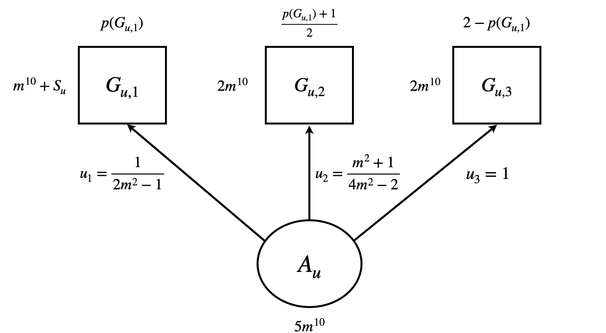
Proof of Lemma 3.10.
Fixing any node , we let denote and to denote the total allocation of to agents in in , for each . We also write to denote the utility of to agents in given in (1). We start by showing that most goods in go to .
Claim 3.17.
We have and .
Proof.
Let and be an optimal solution to the dual LP of agents in . Then for each . We consider the following two cases.
First we consider the case when . This implies that goods outside of are -suboptimal for and thus, by Lemma 3.5, the total allocation of them to agents in is . As a result, from which the claim follows.
Next consider the case when . By Lemma 3.3 () we have for every . This implies that agents with zero utilities to can be allocated only units of given that they are -suboptimal by Lemma 3.4. On the other hand, by Fact 3.9 the allocation to agents outside with positive utilities for is at most . So all the rest of must be allocated to and the claim follows. ∎
Now that we have for all , we proceed to prove (3). Let denote an optimal solution to the dual LP for . By Lemma 3.5 and taking , we have
| (4) |
If this were not the case (i.e. the second inequality is violated for some ), then goods in are -suboptimal to and their total allocation to agents in can be no more than a contradiction.
Next we prove Lemma 3.11:
Proof of Lemma 3.11.
We use the same notation from the proof of the last lemma.
First given that and are , the total allocation of to agents with zero utility on is at most using Lemma 3.5; the same applies to .
Suppose that . Because contains goods while contains only agents, for to be fully sold out, the total allocation of to agents with zero utility on must be . This implies that since otherwise, the total allocation for is at most , using .
3.5 Analysis of Edge Gadgets
In this subsection we prove Lemma 3.12. Let be an -approximate HZ equilibrium of and be an edge in . We work on agents in and to understand their allocations of goods with non-zero utilitites. We start with agents in :

Lemma 3.18.
The allocation of and to each agent in is given by
respectively.
Proof.
The dual LP for each agent in is to minimize subject to the following constraints: ; for ; for ; and for . The constraints for the minimum-priced goods in the groups , dominate the constraints for the others goods in the groups (since ), hence these constraints are equivalent to
| (6) |
The constraint for the good with price yields , and this subsumes the constraints for all . Thus, the dual LP is to minimize subject to , , and (6) above. The optimal solution satisfies the (6) as equalities. Thus, solving the dual LP we get
Consider an agent in and write and respectively to denote her allocation of goods from and . Since every good that is not in is -suboptimal for the agent, it follows from Corollary 3.6 and Corollary 3.15 that
From Lemma 3.10, . For ease of notation, let us use to denote and for . Solving the above equations for and gives us
Since , by performing the first order approximation, we have
The result for can be shown similarly. ∎
Now we work on agents in for each :

Lemma 3.19.
For each , the allocation of goods in to each agent in is if and if .
Proof.
The dual LP of each agent in is to minimize subject to the following constraints: ; ; ; . (We have simplified the dual LP following similar arguments used at the beginning of the proof for the previous lemma.) The optimal solution now has two cases.
Lemma 3.20.
The total allocation of goods in to all agents in , , is
Proof.
Let . Then for each with , the allocation of to each agent in is ; for each with , the allocation is . For and , the allocation is between and trivially.
Since there are 6 agents in each group , the total allocation to all agents in all groups is
The number of summands in the last expression is
and the lemma follows. ∎
The following lemma for agents in can be proved similarly:
Lemma 3.21.
The allocation of goods in to all agents in , , is
Finally we work on agents in , :

Lemma 3.22.
For each , we have the following two cases for an agent in :
- 1.
The allocation of is and the allocation of is , if satisfies
(7) - 2.
The allocation of is and the allocation of is , if satisfies
(8)
Proof.
The dual LP for an agent in is to minimize subject to , ,
| (9) |
Geometrically, the feasible space of the LP is a region of the plane, bounded from below by a a piecewise linear convex curve whose segments correspond to (some of) the above constraints. The optimum is achieved at a vertex of the boundary curve, where the constraints corresponding to the two adjacent segments are tight. We consider the two cases.
First we consider the case of (7). In this case, the first and third inequalities of (9) are tight at optimality, and the optimal solution is
Using (7) and , , it is easy to check that . Therefore, all goods that are not in are -suboptimal. Furthermore, also all goods in are -suboptimal, i.e.,
because multiplying the left-hand-side by we get
So it follows from Lemma 3.5 that the total allocation to the agent (and the cost) of all goods that are not in and is .
Using and to denote the allocation of goods in and to the agent respectively, it follows from Corollary 3.6 and Corollary 3.15 that
and using and , one can derive that .
Similarly, one can show that when (8) holds, then the first two inequalities of (9) are tight at the optimal solution . We have again , and thus all goods outside are -suboptimal. Furthermore, in this case all goods in are also -suboptimal. Hence the total allocation (and cost) of these goods to the agent is . We can set up similarly as in the previous case the equations for the allocations of the goods in , respectively to the agent, and solve them to get . This concludes the proof. ∎
Lemma 3.23.
The total allocation of goods in to agents in , , is
and the total allocation of goods in to these agents is
Proof.
Let be chosen as
We start with goods in . By Lemma 3.22, the total allocation is times
The number of terms in the last sum is
It follows that the total allocation is
Similarly, the total allocation of goods is 18 times
The number of terms in the last sum is
and the lemma follows. ∎
We are now ready to prove Lemma 3.12:
4 Hardness of Approximating Optimal Social Welfare
In this section we study the problem of approximating the optimal social welfare (defined as the total utility of all agents) achievable by an HZ equilibrium. For this purpose we study the following gap problem for a constant : the input is an HZ market together with a parameter SW, and it is promised that the optimal social welfare achievable by an exact HZ equilibrium of is either at least SW or at most . The goal is to tell which case it is. We show that there is no polynomial-time algorithm for the gap problem when , assuming .
Theorem 4.1.
Assuming , for any constant , there is no polynomial-time algorithm for the gap problem when .
4.1 Construction
We reduce from , which is hard to approximate better than [Hås01]: Given a instance, it is NP-hard to distinguish the case that the formula is satisfiable from the case that every truth assignment satisfies at most a fraction of the clauses, for any . Given a instance with clauses and variables, we construct the following HZ market. Throughout the proof, we fix .
Creating Variable Gadget
We first introduce the variable gadget. For convenience, we only list non zero utilities. For each
- 1.
Create three groups of goods , , , and , and .
- 2.
Create two groups of agents , , and .
- 3.
Agents in have utility for , for . Agents in have utility for , for .
In an (exact) HZ equilibrium, all goods within a group have the same price. We use to denote the price, .
Creating Clause Gadget
We next construct clause gadgets. For each ,
- 1.
Create a group of goods
- 2.
Create a group of agents, who have utility for .
- 3.
Create an agent with utility for . It has utility for if the -th clause contains and utility for if the -th clause contains .
Adding Dummy Goods
Thus far, we have described goods and agents. We add extra dummy goods that have zero utilities for all agents. In a normalized (exact) HZ equilibrium, these goods have zero price.
4.2 Proof of Correctness
We provide the proof of completeness and soundness separately.
Completeness
Given a instance that has a satisfying assignment, we construct a HZ equilibrium with social welfare at least . Fix a satisfying assignment.
We assign the -th clause to the -th variable, if the latter satisfies the clause. If there are multiple such variables, we choose an arbitrary one. We set if the -th clause contains , otherwise . Let be the total number of clauses assigned to the -th variable. The equilibrium prices are as follows.
- 1.
The price of dummy goods is .
- 2.
The price of is , .
- 3.
For variable gadget , if , then , otherwise, we have .
Next, we specify the equilibrium allocation.
- 1.
Agents of take of and of dummy goods, .
- 2.
Agent takes of and of , .
- 3.
If , then agents in obtain of , of ; agents in obtain of , of , of and of the dummy good, . If , then we define the allocation symmetrically, switching the groups of agents and , and the groups of goods and .
One can verify that this is indeed a HZ equilibrium. Agent has utility , and hence, the social welfare is at least .
Soundness
Consider any normalized HZ equilibrium . We first characterize the equilibrium behaviour of variable gadgets. In an (exact) HZ equilibrium, we say a variable gadget is vacant if no agents outside of the gadget purchase goods inside the gadget, and we call other gadgets non-vacant. Loosely speaking, only non-vacant gadgets are of interest, as vacant gadgets do not interact with the rest of market and their utility is negligible.
Lemma 4.2.
For any , suppose the -th variable gadget is non-vacant. Then the equilibrium price is one of the following three cases.
| (11) | ||||
| or | (12) | |||
| or | (13) |
Proof.
We have , otherwise is oversold. Since there are outside agents that purchase goods inside the gadget, we conclude that one of the agents in , must purchase goods outside the gadget, i.e. those zero-price zero-utility goods. Assume that some agents in purchase such goods (the other case is symmetric.)
It is easy to see then that , and therefore, the optimal bundles of agents in contain and zero-price zero-utility goods. Hence, . We further divide into two cases based on the optimal bundle of .
First, suppose agents in purchase , and zero-price zero-utility goods. Then we have . Note that there are at most agents outside the gadget that have nonzero utility for or , and no such agents for . Hence, the agents in buy all the goods in the gadget except for at most units of and . Therefore,
Solving the system of this and the previous two equations yields Eq. (13).
Second, suppose agents in only buy , . Suppose . Then we know agents buy of , and therefore, of . Hence, we have
| and | (14) |
These equations, together with yield the same solution, i.e., Eq. (13).
The following lemma follows a similar argument of Lemma 3.16, we omit the proof
Lemma 4.3.
The price of goods satisfies , .
We are now ready to wrap up the proof of soundness. Given an equilibrium that (approximately) maximizes the social welfare, we look at each non-vacant variable gadget. Based on the three cases stated in Lemma 4.2, we extract the -th variable to be if Eq. (12) holds and if Eq. (11) holds. We do nothing for the case of Eq. (13) and those vacant variables (gadgets).
The total utility of all agents in , , and all agents in , is at most . We focus on the utility of agents , . If the -th clause is satisfied, then one of the utility goods has zero price, and one can see that the utility is (at most)
On the other hand, if the -th clause is not satisfied, we still don’t need to consider the vacant gadgets (as there is no interactions), and the utility goods have price at least . Hence the utility is at most
Thus, if the truth assignment satisfies at most clauses then the social welfare is at most
From [Hås01], it is NP-hard to distinguish the case that all clauses can be satisfied (in which case there is an equilibrium with social welfare ) from the case that at most clauses can be satisfied (in which case the maximum social welfare is at most ). The theorem follows.
The construction can be easily modified, if desired, so that all utilities are in , and every agent has minimum utility 0 and maximum utility 1.
5 Discussion
In this paper we resolved the complexity of computing an approximate equilibrium in the Hylland-Zeckhauser scheme for one-sided matching markets: we showed that the problem is PPAD-complete, and this holds even for inverse polynomial approximation and four-valued utilities. We leave open the complexity of exact equilibria, in particular whether the problem is FIXP-complete. Another open question is whether the PPAD-hardness of the approximation problem holds also for 3-valued utilities.
References
- [AJKT17] Saeed Alaei, Pooya Jalaly Khalilabadi, and Eva Tardos. Computing equilibrium in matching markets. In Proceedings of the 2017 ACM Conference on Economics and Computation, pages 245–261, 2017.
- [AS98] Atila Abdulkadiroglou and Tayfun Sonmez. Random serial dictatorship and the core from random endowments in house allocation problems. Econometrica, 66(3):689–702, 1998.
- [BM01] Anna Bogomolnaia and Hervé Moulin. A new solution to the random assignment problem. Journal of Economic theory, 100(2):295–328, 2001.
- [Bud11] Eric Budish. The combinatorial assignment problem: Approximate competitive equilibrium from equal incomes. Journal of Political Economy, 119(6):1061–1103, 2011.
- [CDDT09] Xi Chen, Decheng Dai, Ye Du, and Shang-Hua Teng. Settling the complexity of Arrow-Debreu equilibria in markets with additively separable utilities. In 2009 50th Annual IEEE Symposium on Foundations of Computer Science, pages 273–282. IEEE, 2009.
- [CPY17] Xi Chen, Dimitris Paparas, and Mihalis Yannakakis. The complexity of non-monotone markets. J. ACM, 64(3):20:1–20:56, 2017.
- [CT09] Xi Chen and Shang-Hua Teng. Spending is not easier than trading: on the computational equivalence of Fisher and Arrow-Debreu equilibria. In International Symposium on Algorithms and Computation, pages 647–656. Springer, 2009.
- [DK08] Nikhil R Devanur and Ravi Kannan. Market equilibria in polynomial time for fixed number of goods or agents. In 2008 49th Annual IEEE Symposium on Foundations of Computer Science, pages 45–53. IEEE, 2008.
- [DPSV08] Nikhil R Devanur, Christos H Papadimitriou, Amin Saberi, and Vijay V Vazirani. Market equilibrium via a primal–dual algorithm for a convex program. Journal of the ACM (JACM), 55(5):22, 2008.
- [EMZ19a] Federico Echenique, Antonio Miralles, and Jun Zhang. Constrained pseudo-market equilibrium. arXiv preprint arXiv:1909.05986, 2019.
- [EMZ19b] Federico Echenique, Antonio Miralles, and Jun Zhang. Fairness and efficiency for probabilistic allocations with endowments. arXiv preprint arXiv:1908.04336, 2019.
- [EY10] Kousha Etessami and Mihalis Yannakakis. On the complexity of Nash equilibria and other fixed points. SIAM Journal on Computing, 39(6):2531–2597, 2010.
- [GMVY17] Jugal Garg, Ruta Mehta, Vijay V Vazirani, and Sadra Yazdanbod. Settling the complexity of Leontief and PLC exchange markets under exact and approximate equilibria. In Proceedings of the 49th Annual ACM SIGACT Symposium on Theory of Computing, pages 890–901, 2017.
- [GTV20] Jugal Garg, Thorben Tröbst, and Vijay V Vazirani. An arrow-debreu extension of the Hylland-Zeckhauser scheme: Equilibrium existence and algorithms. arXiv preprint arXiv:2009.10320, 2020.
- [Hås01] Johan Håstad. Some optimal inapproximability results. Journal of the ACM (JACM), 48(4):798–859, 2001.
- [HMPY18] Yinghua He, Antonio Miralles, Marek Pycia, and Jianye Yan. A pseudo-market approach to allocation with priorities. American Economic Journal: Microeconomics, 10(3):272–314, 2018.
- [HZ79] Aanund Hylland and Richard Zeckhauser. The efficient allocation of individuals to positions. Journal of Political economy, 87(2):293–314, 1979.
- [Jai07] Kamal Jain. A polynomial time algorithm for computing an Arrow-Debreu market equilibrium for linear utilities. SIAM J. Comput., 37(1):303–318, 2007.
- [Le17] Phuong Le. Competitive equilibrium in the random assignment problem. International Journal of Economic Theory, 13(4):369–385, 2017.
- [McL18] Andy McLennan. Efficient disposal equilibria of pseudomarkets. In Workshop on Game Theory, volume 4, page 8, 2018.
- [Mou18] Hervé Moulin. Fair division in the age of internet. Annual Review of Economics, 2018.
- [Orl10] James Orlin. Improved algorithms for computing Fisher’s market clearing prices. In Proc. 42nd ACM Symp. Theory of Computing, pages 291–300, 2010.
- [PP21] Christos Papadimitriou and Binghui Peng. Public goods games in directed networks. In Proceedings of the 22nd ACM Conference on Electronic Commerce, 2021.
- [VY11] V. V. Vazirani and M. Yannakakis. Market equilibria under separable, piecewise-linear, concave utilities. Journal of the ACM, 58(3), 2011.
- [VY21] Vijay V Vazirani and Mihalis Yannakakis. Computational complexity of the Hylland-Zeckhauser scheme for one-sided matching markets. In 12th Innovations in Theoretical Computer Science Conference (ITCS 2021). Schloss Dagstuhl-Leibniz-Zentrum für Informatik, 2021.
Appendix A Padding
Recall that the goal is to reduce the problem of finding a -approximate HZ equilibrium to that of finding a -approximate HZ equilibrium, for some constant . Let be an HZ market with goods, agents and utilities . Let . We create a new market with goods and agents. This is done by replacing each good in by a group of goods and replacing each agent in by a group of agents. Agents in each group have the same utility for goods in . Given that is a constant, can be constructed in polynomial time.
Now let be an -approximate HZ equilibrium of with
We derive a pair for the original market as follows: set to be the minimum price of goods in ; set to be the total allocation of goods in to agents in divided by . We prove that is an -approximate HZ equilibrium of . The first two conditions hold trivially by the uniform scaling. For the third condition we note that the total cost of bundles of in is at most . Therefore the cost of the bundle of agent is at most because prices of goods can only go down. For the last property, we note that the utility of agent from is the same as the total utility of agents in divided by . On the other hand, the LP for agent (with respect to ) is the same as the LP for each agent in (with respect to ), after removing subsumed constraints. So they have the same optimal value. This finishes the correctness proof of the reduction.
Appendix B Disconnected Equilibria

We provide a simple example showing that there exists disconnected equilibria even when the HZ market contains only four agents (i.e., ) and the utility is drawn from . The example is indeed the variable gadget we used in Section 4, we present it here for completeness.
Consider the following HZ market. There are two groups of agents, and , and there are three groups of goods, , and . Let , and . Each agent in has utility for goods , utility for goods and utility for goods . Each agent in has utility for goods , utility for goods and utility for goods .
In any (exact) equilibrium, all goods in the same group must clearly have the same price, because otherwise the most expensive good in the group will remain unsold. Let denote an equilibrium price vector of , with . Since both and have utility for , the price , because otherwise will be oversold.
Claim B.1.
There are three disconnected equilibria in the above HZ market, with equilibria prices , and respectively.
Proof.
Since goods and are symmetric, w.l.o.g., we can assume . The optimal bundle of contains exactly goods and in this case, and we know agents purchase unit of goods and unit of goods in total. We conclude since there is at most unit of goods .
When , agents get unit of and unit of , and therefore, agents get unit of and unit of . We have in this case. Thus, the price vector in this case is .
On the other hand, when , the optimal bundle of agent must contain all three goods. Hence, we have and . This leads to and . The equilibrium allocation of equals for agents and for agents . The equilibrium price vector in this case is . Symmetrically, when , there is an equilibrium price vector . ∎
Remark B.2.
If we consider also unnormalized prices (i.e. include price vectors with ), the set of equilibrium price vectors consists of three disjoint regions: , , and . The equilibrium allocations are the same as in the normalized price vectors in the three cases.