Calibrating Predictions to Decisions: A Novel Approach to Multi-Class Calibration

We consider the prediction problem with random variables $X$ and $Y$, where $X\in{\mathcal{X}}$ denotes the input features, and $Y\in{\mathcal{Y}}$ denotes the label. We focus on classification where ${\mathcal{Y}}=\{(1,0,\cdots,0),(0,1,\cdots,0),\cdots,(0,0,\cdots,1)\}$ where each $y\in{\mathcal{Y}}$ is a one-hot vector with $C\in{\mathbb{N}}$ classes. ¹¹ 1 We can also equivalently define ${\mathcal{Y}}=\{1,2,\cdots,C\}$, here we denote $y$ by a one-hot vector for notation convenience when taking expectations. A probability prediction function is a map $\hat{p}:{\mathcal{X}}\to\Delta^{C}$ where $\Delta^{C}$ is the $C$-dimensional simplex. We define the support of ${\hat{p}}$ as the set of distributions it could predict, i.e. $\{{\hat{p}}(x)|x\in{\mathcal{X}}\}$. We use $p^{*}:{\mathcal{X}}\to\Delta^{C}$ to denote the true conditional probability vector, i.e. $p^{*}(x)={\mathbb{E}}[Y\mid X=x]\in\Delta^{C}$, and for all $c\in[C]$, each coordinate gives the probability of the class $p^{*}(x)_{c}=\Pr[Y_{c}\mid X=x]$.

We formalize a decision making task as a loss minimization problem. The decision maker has some set of available actions ${\mathcal{A}}$ and a loss function $\ell:{\mathcal{Y}}\times{\mathcal{A}}\to{\mathbb{R}}$. In this paper we assume the loss function does not directly depend on the input features $X$. For notational simplicity we often refer to a (action set, loss function) pair $({\mathcal{A}},\ell)$ only by the loss function $\ell$: the set of actions ${\mathcal{A}}$ is implicitly defined by the domain of $\ell$. We denote the set of all possible loss functions as ${\mathcal{L}_{\mathrm{all}}}=\{\ell:{\mathcal{Y}}\times{\mathcal{A}}\to\mathbb{R}\}$.

We treat all action sets ${\mathcal{A}}$ with the same cardinality as the same set — they are equivalent up to renaming the actions. A convenient way to think about this is that we only consider actions sets ${\mathcal{A}}\in\{[1],[2],\cdots,[K],\cdots,{\mathbb{N}},{\mathbb{R}}\}$ where $[K]=\{1,\cdots,K\}$.

Given some predicted probability ${\hat{p}}(X)$ on $Y$, a decision maker selects an action in ${\mathcal{A}}$. We assume that the decision maker selects the action based on the predicted probability. That is, we define a decision function as any map from the predicted probability to an action $\delta:\Delta^{C}\to{\mathcal{A}}$. and denote by ${\drule_{\mathrm{all}}}$ as the set of all decision functions.

Typically a decision maker selects the action that minimizes the expected loss (under the predicted probability). This strategy is formalized by the following definition of Bayes decision making.

First and foremost, a decision maker wants assurance that making decisions based on the prediction function ${\hat{p}}$ give low expected loss. In particular, a decision maker with loss $\ell$ wants assurance that the Bayes decision rule $\delta_{\ell}$ is the best decision making strategy, given $\hat{p}$. In other words, she wants $\delta_{\ell}$ to incur a lower loss compared to alternative decision rules. Second, the decision maker wants to know how much loss is going to be incurred (before the actions are deployed and outcomes are revealed); the decision maker does not want to incur any additional loss in surprise that she has not prepared for.

To capture these desiderata we formalize a definition based on the following intuition: suppose a decision maker with some loss function $\ell$ considers a decision rule $\delta\in{\drule_{\mathrm{all}}}$ (that may or may not be the Bayes decision rule), the decision maker should be able to correctly compute the expected loss of using $\delta$ to make decisions, as a function of the predictions $\hat{p}$.

The left hand side of Eq.(2) is the “simulated” loss where the outcome ${\hat{Y}}$ is hypothetically drawn from the predicted distribution. The decision maker can compute this just by knowing the input features $X$ and without knowing the outcome $Y$. The right hand side of Eq.(2) is the true loss that the decision maker incurs in reality if she uses the decision rule $\delta$. Intuitively, the definition captures the idea that the losses in ${\mathcal{L}}$ and decision rules in $\drule$ do not distinguish between outcomes sampled according to the predicted probability and the true probability; specifically, the definition can be viewed as a concrete instantiation of the framework of Outcome Indistinguishability (Dwork et al. 2021).

As a cautionary remark, Eq.(2) should not be mis-interpreted as guarantees about individual decisions; Eq.(2) only looks at the average loss when $X,Y$ is a random draw from the population. Individual guarantees are usually impossible without tools beyond machine learning (Zhao & Ermon 2021). In addition, Definition 2 does not consider decision rules that can directly depend on $X$, as $\delta\in{\drule_{\mathrm{all}}}$ only depends on $X$ via the predicted probability ${\hat{p}}(X)$. Studying decision rules that can directly depend on $X$ require tools such as multicalibration (Hébert-Johnson et al. 2018) which are beyond the scope of this paper (See related work).

In Definition 2 we also define the special notion of ${\mathcal{L}}$-decision calibrated because given a set of loss functions ${\mathcal{L}}$, we are often only interested in the associated Bayes decision rules $\drule_{\mathcal{L}}$, i.e. the set of decision rules that are optimal under some loss function. For the rest of the paper we focus on ${\mathcal{L}}$-decision calibration for simplicity. ${\mathcal{L}}$-decision calibration can capture the desiderata we discussed above formalized in the following proposition.

No regret states that the Bayes decision rule $\delta_{\ell}$ is not worse than any alternative decision rule $\delta^{\prime}\in\drule_{{\mathcal{L}}}$. In other words, the decision maker is incentivized to take optimal actions according to their true loss function. That is, using the predictions given by $\hat{p}$, the decision maker cannot improve their actions by using a decision rule $\delta^{\prime}$ that arises from a different loss function $\ell^{\prime}\in{\mathcal{L}}$.

Accurate loss estimation states that for the Bayes decision rule $\delta_{\ell}$, the simulated loss on the left hand side (which the decision maker can compute before the outcomes are revealed) equals the true loss on the right hand side. This ensures that the decision maker knows the expected loss that will be incurred over the distribution of individuals and can prepare for it. This is important because in most prediction tasks, the labels $Y$ are revealed with a significant delay or never revealed. For example, the hospital might be unable to follow up on the true outcome of all of its patients.

In practice, the forecaster chooses some set ${\mathcal{L}}$ to achieve ${\mathcal{L}}$-decision calibration, and advertise it to decision makers. A decision makers can then check whether their loss function $\ell$ belongs to the advertised set ${\mathcal{L}}$. If it does, the decision maker should be confident that the Bayes decision rule $\delta_{\ell}$ has low loss compared to alternatives in $\drule_{\mathcal{L}}$, and they can know in advance the loss that will be incurred.

We show that by varying the choice of loss class ${\mathcal{L}}$, decision calibration can actually express prior notions of calibration. For example, consider confidence calibration, where among the samples whose the top probability is $\beta$, the top accuracy is indeed $\beta$. Formally, confidence calibration requires that

We show that a prediction function ${\hat{p}}$ is confidence calibrated if and only if it is ${\mathcal{L}}_{r}$-decision calibration, where ${\mathcal{L}}_{r}$ is defined by

Intuitively, loss functions in ${\mathcal{L}}_{r}$ corresponds to the refrained prediction task: a decision maker chooses between reporting a class label, or reporting “I don’t know,” denoted $\bot$. She incurs a loss of $0$ for correctly predicting the label $y$, a loss of $1$ for reporting an incorrect class label, and a loss of $\beta<1$ for reporting “I don’t know”. If a decision maker’s loss function belong to this simple class of losses ${\mathcal{L}}_{r}$, she can use a confidence calibrated prediction function ${\hat{p}}$, because the two desiderata (no regret and accurate loss estimation) in Proposition 1 are true for her. However, such “refrained prediction“ decision tasks only account for a tiny subset of all possible tasks that are interesting to decision makers. Similarly, classwise calibration is characterized through decision calibration using a class of loss functions that penalizes class-specific false positives and negatives.

In this way, decision calibration clarifies the implications of existing notions of calibration on decision making: relaxed notions of calibration correspond to decision calibration over restricted classes of losses. In general, decision calibration provides a unified view of most existing notions of calibration as the following theorem shows.

For proof of this theorem see Appendix C. In Table 1, confidence and classwise calibration are weak notions of calibration; correspondingly the loss function families ${\mathcal{L}}_{r}$ and ${\mathcal{L}}_{\text{cr}}$ are also very restricted.

On the other hand, distribution calibration (i.e. ${\mathbb{E}}[Y\mid{\hat{p}}(X)=q]=q,\forall q\in\Delta^{C}$) is equivalent to ${\mathcal{L}_{\mathrm{all}}}$-decision calibration. This means that a distribution calibrated predictor guarantees the no regret and accurate loss estimation properties as in Proposition 1 to a decision maker holding any loss functions. Unfortunately, distribution calibration is very challenging to verify or achieve. To understand the challenges, consider certifying whether a given predictor ${\hat{p}}$ is distribution calibrated. Because we need to reason about the conditional distribution ${\mathbb{E}}[Y\mid{\hat{p}}(X)=q]$ for every $q$ that ${\hat{p}}$ can predict (i.e. the support of ${\hat{p}}$), the necessary sample complexity grows linearly in the support of ${\hat{p}}$. Of course, for a trivial predictors that map all inputs $x$ to the same prediction $q_{0}$ (i.e. ${\hat{p}}(x)=q_{0},\forall x\in{\mathcal{X}}$) distribution calibration is easy to certify (Widmann et al. 2019), but such predictors have no practical use.

Our characterization of distribution calibration further sheds light on why it is so difficult to achieve. ${\mathcal{L}_{\mathrm{all}}}$ consists of all loss function, including all loss functions $\ell:{\mathcal{Y}}\times{\mathcal{A}}\to{\mathbb{R}}$ whose action space ${\mathcal{A}}$ contains exponentially many elements (e.g. $|{\mathcal{A}}|=2^{C}$). The corresponding decision rules $\delta\in\drule_{{\mathcal{L}_{\mathrm{all}}}}:\Delta^{C}\to{\mathcal{A}}$ may also map $\Delta^{C}$ to exponentially many possible values. Enforcing Definition 2 for such complex loss functions and decision rules is naturally difficult.

In many contexts, directly optimizing for distribution calibration may be overkill. In particular, in most realistic settings, decision makers tend to have a bounded number of possible actions, so the relevant losses come from ${\mathcal{L}}^{K}$ for reasonable $K\in{\mathbb{N}}$. Thus, we consider obtaining decision calibration for all loss functions defined over a bounded number of actions $K$. In the remainder of the paper, we focus on this restriction of decision calibration to the class of losses with bounded action space; we reiterate the definition of decision calibration for the special case of ${\mathcal{L}}^{K}$.

The key result (that we show in Section 4) is that ${\mathcal{L}}^{K}$-decision calibration can be efficiently verified and achieved for all predictors. Specifically, we show that the sample and time complexity necessary to learn ${\mathcal{L}}^{K}$-decision calibrated predictors depends on the number of actions $K$, not on the support of $\hat{p}$. This is in contrast to the standard approach for establishing distribution calibration, which scales with the support of ${\hat{p}}$. Before studying the algorithmic aspects of decision calibration, we argue that ${\mathcal{L}}^{K}$-decision calibration implies similar performance guarantees as distribution calibration to decision makers with bounded actions.

Decision calibration in Definition 2 usually cannot be achieved perfectly. The definition has to be relaxed to allow for statistical and numerical errors. To meaningfully define approximate calibration we must assume that the loss functions are bounded, i.e. no outcome $y\in{\mathcal{Y}}$ and action $a\in{\mathcal{A}}$ can incur an infinite loss. In particular, we bound $\ell$ by its 2-norm $\max_{a}\lVert\ell(\cdot,a)\rVert_{2}:=\max_{a}\sqrt{\sum_{y\in{\mathcal{Y}}}\ell(y,a)^{2}}$. ³³ 3 The choice of 2-norm is for convenience. All $p$-norms are equivalent up to a multiplicative factor polynomial in $C$, so our main theorem (Theorem 2) still hold for any $p$-norms up to the polynomial factor. Now we can proceed to define approximate decision calibration. In particular, we compare the difference between the two sides in Eq.(2) of Definition 2 with the maximum magnitude of the loss function.

Definition 4 is a relaxation of Definition 2: if a prediction function is $({\mathcal{L}},0)$-decision calibrated, then it is ${\mathcal{L}}$-decision calibrated (Definition 2).

The main observation in our paper is that for the set of loss functions with $K$ actions, $({\mathcal{L}}^{K},\epsilon)$-decision calibration can be verified and achieved with polynomially many samples.

As with distribution calibration, trivial predictors ${\hat{p}}(x)\equiv{\mathbb{E}}[Y],\forall x$ satisfy $({\mathcal{L}}^{K},0)$-decision calibration. To maintain a meaningful prediction function we also require “sharpness” which we measure by $L_{2}$ error. We guarantee that the $L_{2}$ error of ${\hat{p}}^{\prime}$ can only improve under post-processing; that is, ${\mathbb{E}}[\lVert{\hat{p}}^{\prime}(X)-Y\rVert_{2}^{2}]\leq{\mathbb{E}}[\lVert{\hat{p}}(X)-Y\rVert_{2}^{2}]$. In fact, the algorithm works by iteratively updating the predictions to make progress in $L_{2}$. For rest of this section, we propose concrete algorithms that satisfy Theorem 2.

This section focuses on the first part of Theorem 2 where we certify $({\mathcal{L}}^{K},\epsilon)$-decision calibration. A naive approach would use samples to directly estimate

and compare it with $\epsilon$. However, the complexity of this optimization problem poses challenges to analysis. We will make several observations to transform this complex optimization problem to a simple problem that resembles linear classification.

This section discusses the second part of Theorem 2 where we design a post-processing recalibration algorithm. The algorithm is based on the following intuition, inspired by (Hébert-Johnson et al. 2018): given a predictor ${\hat{p}}$ we find the worst $b\in B^{K}$ that violates Eq.(8) (line 3 of Algorithm 1); then, we make an update to ${\hat{p}}$ to minimize the violation of Eq.(8) for the worst $b$ (line 4,5 of Algorithm 1). This process is be repeated until we get a $(B^{K},\epsilon)$-decision calibrated prediction (line 2). The sketch of the algorithm is shown in Algorithm 1 and the detailed algorithm is in the Appendix.

Given a dataset with $N$ samples, the expectations in Algorithm 1 are replaced with empirical averages. The following theorem demonstrates that Algorithm 1 satisfies the conditions stated in Theorem 2.

The theorem demonstrates that if we can solve the inner search problem over $B^{K}$, then we can obtain decision calibrated predictions efficiently in samples and computation.

We complete the discussion by addressing the open computational question. Directly optimizing over ${B^{K}}$ is difficult, so we instead define the softmax relaxation.

The key motivation behind this relaxation is that $\bar{b}_{w}\in{\bar{B}^{K}}$ is now differentiable in $w$, so we can optimize over ${\bar{B}^{K}}$ using gradient descent. Correspondingly some technical details in Algorithm 1 change to accommodate soft partitions; we address these modifications in Appendix A and show that after these modifications Theorem 2.2 still holds. Intuitively, the main reason that we can still achieve decision calibration with softmax relaxation is because ${B^{K}}$ is a subset of the closure of ${\bar{B}^{K}}$. Therefore, compared to Eq.(8), we enforce a slightly stronger condition with the softmax relaxation. This can be formalized in the following proposition.

We remark that unlike Proposition 3 (which is an “if and only if” statement), Proposition 4 is a “if” statement. This is because the closure of $\bar{B}^{K}$ is superset of $B^{K}$, so Eq.(9) implies Eq.(8) but not vice versa.

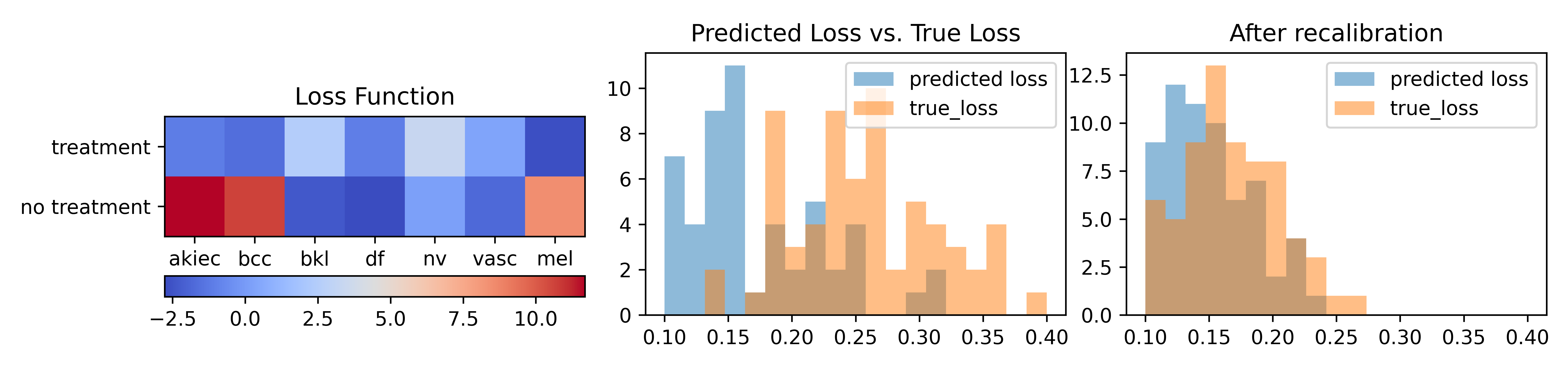
This experiment materializes our motivating example in the introduction. We aim to show on a real medical prediction dataset, our recalibration algorithm improves both the decision loss and reduces the decision loss estimation error. For the estimation error, as in Definition 4 for any loss function $\ell$ and corresponding Bayes decision rule $\delta_{\ell}$ we measure

In addition to the loss function in Figure 1 (which is motivated by medical domain knowledge), we also consider a set of 500 random loss functions where for each $y\in{\mathcal{Y}},a\in{\mathcal{A}}$, $\ell(y,a)\sim\text{Normal}(0,1)$, and report both the average loss gap and the maximum loss gap across the loss functions.

We stress test our algorithm on Imagenet. The aim is to show that even with deeply optimized classifiers (such as inception-v3 and resnet) that are tailor made for the Imagenet benchmark and a large number of classes (1000 classes), our recalibration algorithm can improve the loss gap in Eq.(10).

References

- Barber et al. (2019) Rina Foygel Barber, Emmanuel J Candes, Aaditya Ramdas, and Ryan J Tibshirani. The limits of distribution-free conditional predictive inference. arXiv preprint arXiv:1903.04684, 2019.
- Brier (1950) Glenn W Brier. Verification of forecasts expressed in terms of probability. Monthly weather review, 78(1):1–3, 1950.
- Dawid (1984) A Philip Dawid. Present position and potential developments: Some personal views statistical theory the prequential approach. Journal of the Royal Statistical Society: Series A (General), 147(2):278–290, 1984.
- Dwork et al. (2019) Cynthia Dwork, Michael P Kim, Omer Reingold, Guy N Rothblum, and Gal Yona. Learning from outcomes: Evidence-based rankings. In 2019 IEEE 60th Annual Symposium on Foundations of Computer Science (FOCS), pp. 106–125. IEEE, 2019.
- Dwork et al. (2021) Cynthia Dwork, Michael P Kim, Omer Reingold, Guy N Rothblum, and Gal Yona. Outcome indistinguishability. STOC, 2021.
- Fang et al. (1994) Yuguang Fang, Kenneth A Loparo, and Xiangbo Feng. Inequalities for the trace of matrix product. IEEE Transactions on Automatic Control, 39(12):2489–2490, 1994.
- Guo et al. (2017) Chuan Guo, Geoff Pleiss, Yu Sun, and Kilian Q Weinberger. On calibration of modern neural networks. In International Conference on Machine Learning, pp. 1321–1330. PMLR, 2017.
- Hébert-Johnson et al. (2018) Ursula Hébert-Johnson, Michael Kim, Omer Reingold, and Guy Rothblum. Multicalibration: Calibration for the (computationally-identifiable) masses. In International Conference on Machine Learning, pp. 1939–1948. PMLR, 2018.
- Huang et al. (2017) Gao Huang, Zhuang Liu, Laurens Van Der Maaten, and Kilian Q Weinberger. Densely connected convolutional networks. In Proceedings of the IEEE conference on computer vision and pattern recognition, pp. 4700–4708, 2017.
- Jung et al. (2020) Christopher Jung, Changhwa Lee, Mallesh M Pai, Aaron Roth, and Rakesh Vohra. Moment multicalibration for uncertainty estimation. arXiv preprint arXiv:2008.08037, 2020.
- Kim et al. (2019) Michael P Kim, Amirata Ghorbani, and James Zou. Multiaccuracy: Black-box post-processing for fairness in classification. In Proceedings of the 2019 AAAI/ACM Conference on AI, Ethics, and Society, pp. 247–254, 2019.
- Kleinberg et al. (2016) Jon Kleinberg, Sendhil Mullainathan, and Manish Raghavan. Inherent trade-offs in the fair determination of risk scores. arXiv preprint arXiv:1609.05807, 2016.
- Kuleshov et al. (2018) Volodymyr Kuleshov, Nathan Fenner, and Stefano Ermon. Accurate uncertainties for deep learning using calibrated regression. In International Conference on Machine Learning, pp. 2796–2804. PMLR, 2018.
- Kull & Flach (2015) Meelis Kull and Peter Flach. Novel decompositions of proper scoring rules for classification: Score adjustment as precursor to calibration. In Joint European Conference on Machine Learning and Knowledge Discovery in Databases, pp. 68–85. Springer, 2015.
- Kull et al. (2019) Meelis Kull, Miquel Perello-Nieto, Markus Kängsepp, Hao Song, Peter Flach, et al. Beyond temperature scaling: Obtaining well-calibrated multiclass probabilities with dirichlet calibration. arXiv preprint arXiv:1910.12656, 2019.
- Mohri et al. (2018) Mehryar Mohri, Afshin Rostamizadeh, and Ameet Talwalkar. Foundations of machine learning. MIT press, 2018.
- Platt et al. (1999) John Platt et al. Probabilistic outputs for support vector machines and comparisons to regularized likelihood methods. Advances in large margin classifiers, 10(3):61–74, 1999.
- Pleiss et al. (2017) Geoff Pleiss, Manish Raghavan, Felix Wu, Jon Kleinberg, and Kilian Q Weinberger. On fairness and calibration. In Advances in Neural Information Processing Systems, pp. 5680–5689, 2017.
- Shabat et al. (2020) Eliran Shabat, Lee Cohen, and Yishay Mansour. Sample complexity of uniform convergence for multicalibration. NeurIPS, 2020.
- Song et al. (2019) Hao Song, Tom Diethe, Meelis Kull, and Peter Flach. Distribution calibration for regression. In International Conference on Machine Learning, pp. 5897–5906. PMLR, 2019.
- Tschandl et al. (2018) Philipp Tschandl, Cliff Rosendahl, and Harald Kittler. The ham10000 dataset, a large collection of multi-source dermatoscopic images of common pigmented skin lesions. Scientific data, 5(1):1–9, 2018.
- Widmann et al. (2019) David Widmann, Fredrik Lindsten, and Dave Zachariah. Calibration tests in multi-class classification: A unifying framework. arXiv preprint arXiv:1910.11385, 2019.
- Zhao & Ermon (2021) Shengjia Zhao and Stefano Ermon. Right decisions from wrong predictions: A mechanism design alternative to individual calibration. In International Conference on Artificial Intelligence and Statistics, pp. 2683–2691. PMLR, 2021.
- Zhao et al. (2020) Shengjia Zhao, Tengyu Ma, and Stefano Ermon. Individual calibration with randomized forecasting. arXiv preprint arXiv:2006.10288, 2020.
Appendix A Relaxations to Decision Calibration
We define the algorithm that corresponds to Algorithm 1 but for softmax relaxed functions. Before defining our algorithm at each iteration we first lighten our notation with a shorthand (at different iteration , denotes different functions), and is the vector of .
For the intuition of the algorithm, consider the -th iteration where the current prediction function is . On line 4 we find the worst case that maximizes the “error” , and on line 5-7 we make the adjustment to minimize this error . In particular, the adjustment we aim to find on line 5-7 (which we denote by ) should satisfy the following: if we let
we can minimize
We make some simple algebra manipulations on to get
Suppose is invertible, then the optimum of the objective is
When is not invertible we can use the pseudo-inverse, though we observe in the experiments that is always invertible.
For the relaxed algorithm we also have a theorem that is equivalent to Theorem 2.2. The statement of the theorem is identical; the proof is also essentially the same except for the use of some new technical tools.
Appendix B Additional Experiment Details and Results
Additional experiments are shown in Figure 4 and Figure 5. The observations are similar to those in the main paper.