Constraints on pure point diffraction on aperiodic point patterns of finite local complexity
Abstract
It is shown that the partial amplitudes of the pure point part of the diffraction spectrum of an aperiodic Delone point pattern of finite local complexity are linked by a set of linear constraints. These relations can be explicitly derived from the geometry of the prototile space of the underlying tiling.
1 Introduction
Delone sets of finite local complexity (FLC) are traditional objects of study in the diffraction theory of aperiodic solids. In this paper, instead of considering individual Delone sets which just happen to have the FLC property, we rather deal with families of such sets, having common allowed local configurations, and study the constraints on the pure point diffraction stemming from these local rules. The main motivation of this approach comes from the problem of the structural analysis in quasicrystals and is explained in details in [1]. However, in contrast with [1], this paper is not limited to the case of the quasiperiodic long-range order. Neither the restrictions on local environments need to have the strength of the matching rules, that is fix by themselves the long-range order of the structure. In particular, the results are also applicable to the pure point part of diffraction of random tiling models.
The results of this paper are formulated in terms of the partial diffraction amplitudes of the following distribution associated with an FLC Delone multiset in the Euclidean space :
| (1) |
where the index enumerates atomic sites distinguished by their local environment and the weights represent their diffractive power. The partial amplitudes will be properly defined in Proposition 2, but it is reasonable to think of them informally as of the following quantities:
| (2) |
where is the wave vector corresponding to a Bragg peak and is the ball of radius centered at the origin. The hypothesis that the pure-point part of the diffraction measure of the distribution (1) is related to the amplitudes (2) by the formula
| (3) |
is commonly known as Bombieri-Taylor conjecture [2].
We shall consider the sets in (1) as decorations of a tiling in , and treat the corresponding prototile space as the embodiment of the local rules. In this setting, the informal expression (2) offers a glimpse of the nature of the constraints on the partial diffraction amplitudes , considered as functions on the prototile space. Indeed, as moving the decorating point within a prototile shifts the entire set and thus modifies (2) by a phase factor, all these functions belong to a finite-dimensional linear space. Furthermore, since the decoration at a tile boundary can be assigned to either of the neighboring tiles, the partial amplitudes are subject to additional linear constraints akin to the Kirchhoff’s current conservation law.
The paper is organized as follows. Section 2 sets up the model of Delone multisets of finite local complexity in terms of flat-branched semi-simplicial complexes and isometric windings. Section 3 is devoted to a formal definition of the partial diffraction amplitudes in terms of dynamical systems. The main results of the paper (Theorem 1 and Corollary 2) are exposed in Sections 4 and 5. Finally, Section 6 illustrates these results by several examples of aperiodic point patterns.
2 The model
A convenient way to impose local rules on the multiset in (1) consists in treating it as a decoration of a tiling of . The range of the local rules is not limited by the tiles sizes, since the environment on a longer range can always be specified by discrete labels attached to the tiles. Without loss of generality, we can limit the consideration to the case of simplicial tilings. Note, that contrary to a common usage, we treat such a tiling as a partition of by a countable set of interiors of affine simplices, in particular we accept simplicial tiles of any dimension from to (by a common convention, a vertex is its own interior). A class of tiles identically labeled and having the same shape (up to a translation) is called a prototile (this term may also refer to an arbitrary representative of the class). One can introduce an order on the vertices of each prototile by choosing a direction in not orthogonal to any prototile edge, and ordering vertices by the values of their projections on this direction. Then the face of a prototile is defined as its face not containing the vertex. Let stand for the set of prototiles of dimension . The matching constraints on the tiles are realized by defining the maps assigning to each the prototile glued to its face. Since the ordering of vertices remains consistent across dimensions, the maps satisfy the simplicial identity (54). We shall denote the resulting semi-simplicial set (see Appendix A) by . The corresponding geometric realization thus represents the prototile space of the tiling.
In addition to the combinatorial data encoded by , the local rules must also specify the geometry of prototiles, which can be recovered from the directions and orientations of edges. The latter are constrained by the condition that the edges of each face of a prototile form a triangle. This constraint can be conveniently formulated in terms of the chain complex (see Appendix A), leading to the following definition [1]:
Definition 1.
A flat-branched semi-simplicial complex (FBS-complex) is a triple , where is a finite semi-simplicial set of dimension , is a real Euclidean vector space and is a homomorphism satisfying the following conditions:
- •
The homomorphism vanishes on boundaries.
- •
For any , the vectors are linearly independent.
For any let be given by the formula
| (4) |
The second condition of Definition 1 guarantees that is a non-degenerate affine simplex. Identification of barycentric coordinates within and defines a homeomorphism
| (5) |
The tilings obeying the matching rules encoded by an FBS-complex are in one-to-one correspondence with the isometric windings of the latter [1]:
Definition 2.
A continuous map is called isometric winding of an FBS-complex if
- •
For each the restriction is a covering map of .
- •
The composition restricted to any connected component of is a translation of by some vector of .
The tiling corresponding to an isometric winding is given by the partition of by connected components of for all . Fixing a point defines a decoration of this tiling by the set . We shall use this construction to define the sets in (1) by fixing points and setting . This leads to the following formula for the distribution of the diffracting quantity:
| (6) |
The formula (6) describes the model of the distribution of matter which will be used throughout the rest of the paper.
3 Partial diffraction amplitudes
The main flaw of the informal expression (2) is the presence of the limit operation, which makes proving any result about a daunting task. The crucial step towards a closed expression for the diffraction amplitudes consists in using the theory of dynamical systems. The key element in this scheme is the hull of the diffracting distribution – a compact topological space representing arbitrarily large finite patches of an infinite system “all at once”. The idea to use the hull in studying diffraction has been proposed by Dworkin in [3], and since then has lead to a significant progress in understanding the relation between the diffraction and dynamical spectra ([4, 5, 6]). In this section, we follow mostly the ideas of [4] and [7], but with the twist of using a matrix-valued diffraction measure.
In the theory of aperiodic order, hulls are built by adding limiting points to the orbit of an aperiodic structure under the action of translations. The actual construction may come in different guises, either as a closure of the orbit in an appropriate topological vector space (for the hulls of almost periodic functions or measures), or as a completion of the orbit in appropriate metric (in the case of point sets or tilings [8]). Since we shall be mostly interested in the dependence of the pure point component of the diffraction measure on the parameters and in (6) (cf. the formula (20) below), the construction of the hull should depend only on the properties of the isometric winding in (6). The translation of the diffracting distribution by a vector corresponds to the following transformation of :
| (7) |
For a given isometric winding we shall define its hull as the closure of its orbit in the compact-open topology of :
| (8) |
Let us show that this construction is equivalent to that of the tiling space (a continuous hull) [8] of . Consider the patch of a shifted tiling contained within a compact window . Since has finite local complexity, there exists a compact such that all these patches are generated by shifts . Therefore
| (9) |
Since the right-hand side of (9) is an image of the compact , the left-hand side is closed in the compact-open topology of . Thus, for any there exists such that . Therefore all points of are isometric windings and thus correspond to tilings, while the convergence in is equivalent to that in the tiling space of .
The closed formula for the partial diffraction amplitudes requires one more ingredient – a translation invariant probability measure on . Such a measure always exists since is compact, but it may be not unique. Although the results of this section remain valid for any translation invariant measure, it should be emphasized that the well-definedness of the limit in the formula (2) is guaranteed only in the case when there exists only one such measure, that is when the measure-preserving dynamical system is uniquely ergodic [9]. On the other hand, in real physical applications the condition of unique ergodicity is not very stringent since it corresponds to an intuitive notion of macroscopic uniformity of the specimen. Bearing this in mind we shall treat the measure as a background parameter and omit to reference it unless necessary.
Let stand for the Schwartz space on . For a given point , let be the linear map defined by the formula
| (10) |
Since is rapidly decreasing and is uniformly discrete, the sum in the above expression converges absolutely, therefore is continuous. Consider the following sesquilinear functional on (we use the convention that Dirac bracket is antilinear in the first argument):
This functional is translationally invariant, positive definite and continuous in each argument. Therefore (see [10, Chapter II.3, Theorem 6] and the discussion afterwards), there exists a positive tempered measure on such that
| (11) |
We shall take (11) as the definition of the diffraction measure of the distribution (6) (see Appendix B for the proof that this definition is equivalent to more traditional ones).
The diffraction measure in (11) is sesquilinear in the weights :
| (12) |
where are complex-valued tempered measures on . It is convenient to consider them as elements of a matrix-valued measure on
The values of on bounded Borel sets of are Hermitian positive semi-definite matrices.
We shall now follow the ideas of [4] and construct the isometric embedding of Hilbert spaces
| (13) |
where stands for the space of (classes of) functions square-integrable with respect to the matrix-valued diffraction measure (see [11] for the details). Let as start by defining the action of on the Schwartz space by the formula
| (14) |
where and stands for the canonical basis in . As follows from (11) and (12), intertwines the inner product of restricted to with that of . The isometric embedding (13) is then defined as the continuous extension the map (14) to , which is unique by virtue of the following proposition:
Proposition 1.
is dense in
Proof.
Let us denote the scalar measure given by the trace of by and consider as a space of classes of functions on . Since is non-negative, the norm of is stronger than that of . This defines a continuous linear map
| (15) |
As follows from [11, Theorem 3.11], simple functions are dense in . By standard arguments so are also the simple functions with compact support. Since is locally finite, the latter belong to the image of (15), which is therefore dense in . Let stand for the space of continuous functions with compact support. These functions are approximated by those of uniformly, and thus also in the norm of . It remains to show that is dense in , which follows immediately from [12, Theorem 3.14]. ∎
Let us show now that the isometric embedding (13) is equivariant with respect to translations of . For any let stand for the unitary operator on defined by the formula
| (16) |
where and . The translation also acts on by the unitary operator :
where , and is given by the formula (7). In particular, for in (10) we have
| (17) |
where . Therefore, as follows from (14)
Then, by virtue of Proposition 1, the identity
| (18) |
holds on the entire Hilbert space . In other words, the isometric embedding (13) intertwines the action of on by with that on by .
The notable consequence [4, 6, 7] of the identity (18) is that the pure point part of the diffraction measure is a subset of the pure-point part of the dynamical spectrum of , which is defined as the set of values for which there exists a non-zero eigenfunction :
While the dependence of the diffraction measure on the weights in (6) is captured by the matrix-valued measure , the latter still depends on the positions of the atomic decorations . The following result shows that the pure-point part of the diffraction measure can be expressed in terms of individual contributions of each atomic site , thus justifying the formula (3):
Proposition 2.
Let be an isometric winding and let be a translationally invariant probability measure on its hull . Then for any eigenvalue and a corresponding normalized eigenfunction there exists a (not necessarily continuous) function such that for any set of atomic decorations in (6) holds the identity
| (19) |
Moreover, if is ergodic, one also has
| (20) |
We shall refer to the functions as the partial diffraction amplitudes of the dynamical system .
Proof.
Let us consider the distribution defined by the formula
Using (17) we get
hence satisfies the following equation:
| (21) |
The solutions of this equation in have the form
where is an arbitrary complex constant. Therefore there exists a function such that
| (22) |
for any and any . Then as follows from (14)
| (23) |
Since the multiplication by in is the projector on the eigenspace of (16), the embedding intertwines it with the projector on the corresponding eigenspace of and we have
4 Constraints on partial amplitudes of a single Bragg peak
We are now going to study the behavior of the partial amplitudes as functions on . The results can be conveniently formulated in terms of semi-simplicial vector spaces (see Appendix A)11 1 In the case when the semi-simplicial set describes a regular cellular complex the results of Sections 4 and 5 can also be formulated in terms of homology of cellular cosheaves [13] on . While this approach might be more natural for the case of no-simplicial tilings, it is not immediately applicable to some relevant examples when the cellular complex associated with is not regular.. Let us start by constructing a family of such spaces parameterized by a vector .
Let be the space of functions spanned by , where
| (24) |
Since all functions are linearly independent, they form a basis of the direct sum
which is naturally a subspace of the space of all complex-valued functions on .
Proposition 3.
Let be the partial diffraction amplitudes defined in Proposition 2. Then for any
| (25) |
Proof.
Let us now provide the graded vector space with the face operators , defined via the face maps as:
| (26) |
where and is given by
| (27) |

Note that with the expression (27) for , the affine simplex is the face of the affine simplex for any (see Figure 1). Consequently, the linear operator in (26) acts on the basis function by its continuation to the face of . Therefore, the operators satisfy the simplicial identity (54) and provide with the structure of a semi-simplicial vector space which we shall denote by .
To formulate the main result of this section, we shall need an orientation of , which can be introduced by fixing a non-zero constant :
| (28) |
Let be defined as
Theorem 1.
Let be the partial diffraction amplitudes defined in Proposition 2. Then for any , the function is a of the chain complex :
| (29) |
Proof.
Note first that since by Proposition 3 and is constant on all of and zero elsewhere, we have . To prove the cycle condition (29) it suffices to show that vanishes on any . As follows from (26), the values of on depend only on the values of on the neighboring of . Let us denote the set of those neighbors (considered together with the index of the face corresponding to ) by :
As follows from (24) and (26), for any and for any points and one has
| (30) |
The identity (30) allows to express the value of at a point via the values of at arbitrarily chosen points (one for each ):
| (31) |
To finish the proof, we shall use an appropriate choice of the points to show that that the right-hand side of (31) is zero.
For any , the affine simplex has as its face. Let us denote the opposite vertex of by . The hyperplane of containing divides the set of points in two parts, following the sign of the expression
| (32) |
The set is thus naturally split as , according to the sign of (32). As follows from (27), the position of is given by the formula
To compute the sign of (32) one can use the identity
together with (28), which gives rise to
Let and stand for the intersections of the affine simplices for belonging to and respectively:
| (33) |

(see Figure 2). Both and are non-empty open polyhedra having as a face. Therefore, one can choose a vector such that and fix the points in (31) in such a way such that
| (34) |
The formula (31) then yields
| (35) |
where
Note now that as follows from (34), if and only if for any isometric winding . In other words,
and for any
Then, as follows from (21)
| (36) |
and the terms at the right-hand side of (35) cancel each other, which proves (29). ∎
As follows from the equations (25) and (29), the functions restricted to the simplices of belong to a linear space of dimension not exceeding . On the other hand, as can be seen from (36), the values of on the simplices of dimension depends linearly on those on the neighboring simplices. The reasoning leading to (36) can be easily generalized to simplices of lower dimensions. Therefore, if the number of atomic positions in the model (6) is big enough, the contributions of these positions in the pure point diffraction are subject to linear constraints:
Corollary 1.
There exist at least linear constraints on the partial amplitudes .
5 Bragg peaks densely filling a subspace
Let be a non-zero linear subspace of . We are going now to establish a connection between constraints on partial amplitudes of different Bragg peaks in the case where is dense in an open subset of , and this is the second main result of this paper. Let us start by showing that the semi-simplicial vector spaces for any can be obtained by an appropriate extension of scalars from only one semi-simplicial module.
Let us denote by the image of the group homomorphism given by the formula
| (37) |
For , let stand for the ring homomorphism extending the following character of :
| (38) |
and let stand for the functor of extension of scalars by .
Proposition 4.
There exists a semi-simplicial such that for any the semi-simplicial vector space is isomorphic to .
Proof.
We shall define by providing an ordinary free graded over the formal basis with the face homomorphisms. Let us start by fixing an element and associating with each an arbitrarily chosen satisfying the condition
| (39) |
(this is always possible since is connected). The face homomorphisms of are defined via the face maps as follows:
| (40) |
where and is given by
(this expression is well-defined since in both cases the arguments of are cycles). To check that is indeed a semi-simplicial , it remains to verify that the homomorphisms (40) satisfy the simplicial identity (54). This result stems from the following identity in :
| (41) |
(note that we use the multiplicative notation for the action of as an element of the group ring in (40) and the additive notation for the group operation in in (41)).
Let be the basis in corresponding to . The functorial image of the face homomorphisms is then given by the following formula:
Consider now the bijective linear map defined by its action on the basis :
| (42) |
where is defined in (24) and the unitary factors are given by
| (43) |
As follows from the identity
commutes with the face operators and is therefore an isomorphism of semi-simplicial vector spaces and . ∎
Proposition 5.
Let be a generating set of of (which can always be chosen finite since is a Noetherian ring) and let be the coefficients of the cycle in the basis of :
Then for almost all with the possible exception of a nowhere dense subset of , the space of of is spanned by the set of vectors
| (44) |
where the phase factors are given by (43)).
Corollary 2.
For any linear subspace , there exists a finite set of smooth functions indexed by a generating set of the of , such that for almost all (with the possible exception of a subset nowhere dense in ), the vector of partial diffraction amplitudes defined in Proposition 2 belongs to a subspace spanned by .
As follows from (24), (43) and (44), the components of are finite exponential sums of the form
| (45) |
where is a finite subset of , and . It is remarkable that while the dependence of the diffraction amplitudes on is usually utterly irregular, the constraints (45) for the partial amplitudes are smooth functions of . Note, however, that these constraints are effective only if the Bragg peaks fill densely an open subset of and when the number of distinct atomic sites in (6) is large enough (e.g. if exceeds the number of generators of the of ).
To prove Proposition 5 we shall need the following technical result:
Proposition 6.
If is a homomorphism of free , then for all
Moreover, the subset for which this inequality is strict
is nowhere dense in .
Proof.
Let . Since is a commutative domain, the rank of a homomorphism of free modules coincides with that of its matrix over the quotient field of [14, Ex. 5.23A]. Hence, all minors of order of the matrix of (if any) are zero, and there exists a non-zero minor of order . All these minors are elements of and the corresponding minors of are obtained from them by the ring homomorphism . Therefore, for any . Let be a non-vanishing minor of of order . Then the expression
defines an entire analytic function on vanishing on and thus also on the closure of in . If this closure contains an open subset of , this function is zero. Since the set of functions
is linearly independent, . This contradiction proves the Proposition. ∎
Proof of Proposition 5.
Consider the homomorphism mapping each basis element of the free over the set to the corresponding element of . Since is the generating set of the submodule of , the following sequence of free
| (46) |
is exact. Applying the extension of scalars to (46) yields the upper row of the following diagram (which is commutative by Proposition 4):
| (47) |
Since the sequence (46) remains exact when extended to the vector spaces over the quotient field, one has
Then by Proposition 6, for all holds the equality
and thus the rows of (47) are also exact. As follows from (42), the vectors of the set (44) are images of the the basis vectors of in the bottom row of (47). Therefore, for all the subspace of in is spanned by (44). Since is nowhere dense in , this proves the Proposition. ∎
In the physically relevant case where (and therefore can be considered as a subgroup of ), is possible to give a geometric meaning to formula (45) in the following way. Since is a quotient of by the kernel of (37), there exists a normal semi-simplicial covering for which is the group of deck transformations. The corresponding action of on commutes with the face homomorphisms and therefore defines on the structure of a semi-simplicial . It is straightforward to check using formula (40) that this module is isomorphic to . Hence, the of can be seen as formal finite integer linear combinations of copies of prototiles translated by vectors of . The of (and thus also those of ) then correspond to the combinations with boundaries canceling out. The advantage of this approach is that it can be directly applied to tilings with tiles of arbitrary shapes, without preliminary triangulation, as illustrated by Figure 3. This representation can be used directly to calculate the sum at the right hand side of (45). Assuming that Figure 3 depicts the cycle , and the decoration corresponds to the point , the vectors in (45) are given by the positions of the copies of the decorating point, and the coefficients are the weights of the corresponding tiles ( and for the case shown on Figure 3).

6 Examples
6.1 Binary patterns in one dimension
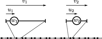
One-dimensional binary patterns are decorated tilings of the real line by two types of intervals. Let and stand for the length of the intervals and let and be the positions of the decorating points (relative to the left end of the respective intervals). The diffracting distribution (1) of a binary pattern is defined by assigning complex weights and to the respective decorations (see Figure 4).
Let us now describe the FBS-complex encoding the binary patterns. The graded set contains three elements:
with the face maps given by
Therefore, the geometric realization of the semi-simplicial set is a bouquet of two circles (see Figure 5). The group of of is generated by the one-dimensional simplices and . Finally, the homomorphism is defined by the formula
(recall that in this case is a real line).

Let us now assume that the set of Bragg peaks of the considered binary pattern is dense in . With the notation used in of Section 5, this amounts to the assumption that with naturally isomorphic to . Therefore, the group (see (37)) is generated by and .
Let us first consider the case when and are commensurate, that is there exists such that
where are coprime. In this case is a free abelian group of rank 1 generated by . It is convenient to write the group operation in multiplicative notation, and treat the group ring as a ring of Laurent polynomials:
where the multiplication by the indeterminate corresponds to the action of . Since contains only one vertex, one can set in (39) for all . Then the face homomorphisms (40) of take the following form
The generating set of Proposition 5 contains only one cycle with the coefficients
Therefore, the partial amplitudes and for all Bragg peaks with the exception of a nowhere dense set obey the following constraint:
valid for . In the case and this amounts to , which reflects the trivial fact that for in this case one recovers the periodic Dirac comb.
When and are incommensurate, is a free abelian group of rank 2 generated by and . Again, we shall use the multiplicative notations
with the multiplication by the indeterminate corresponding to the action of . The face homomorphisms (40) are then given by
and again, contains a single cycle with the coefficients
leading to the following constraint
valid for .
6.2 Decorated canonical tilings
Let us fix vectors , such that any of them are linearly independent over . The prototiles of an tiling [15] of are parallelotopes with edges (one prototile for every subset ). For the sake of simplicity we shall limit the consideration to the case when are linearly independent over and shall also assume that the Bragg peaks are dense in .
The results of this paper are not directly applicable to canonical tilings for since the prototiles are not simplices. However, as a parallelotope can be straightforwardly triangulated by simplices, we shall tacitly assume such triangulation applied to every tile. As follows from (25), partial diffraction amplitudes at the points belonging to the same simplex are related by a trivial phase factor. Since the triangulation of a prototile is purely formal, the same applies to the points belonging to the same prototile of the canonical tiling. To keep focus on the non-trivial constraints only, we shall therefore consider only the case when each prototile is decorated by a single point at its center (see Figure 6).


Similarly to the previous example, we assume . The group is then freely generated by and we shall use the multiplicative notation for the ring :
The space of the FBS-complex of an tiling is a (triangulated) of the standard CW-decomposition of an torus . We can use this fact to calculate the homology of the chain complex in the following way. For , let stand for the chain complex of free of rank 1:
| (48) |
The complex is isomorphic to the complex of submodules of corresponding to the the edge and the unique vertex of . The CW-decomposition of the entire torus then corresponds to the tensor product of over for :
| (49) |
Note that (49) is naturally a complex of modules over the ring
| (50) |
The of the torus is described by the truncated chain complex
| (51) |
The triangulation of the prototiles of the canonical tiling thus yields a chain quasi-isomorphism (see e.g. [16, Chapter 1.1]) of (51) to . Since the chain complex (48) is acyclic, so is and the of the truncated complex (51) are precisely the boundaries of the of . Therefore, the module of of is a free of rank . Taking into account that an tiling has prototiles, the constraints of Corollary 2 are effective in the case .
It is instructive to consider in details the case . In this situation, the generating set of of contains only one element. Therefore, the partial amplitudes at decorating points must belong to a one-dimensional subspace of , depending smoothly on . Let us denote by the decorating point belonging to the prototile not having as its edge (see Figure 6(b)). A straightforward computation (using the approach presented at the end of Section 5) then leads to the following formula for the partial amplitudes:
where the coefficient depends on the tiling under consideration and is clearly not a regular function of .
6.3 Decorated square-triangle tiling
The square-triangle tiling is a popular model for the structure of planar aperiodic systems with twelve-fold symmetry. It describes remarkably well the quasiperiodic order observed in molecular dynamics simulation [17], and has also attracted attention recently in soft mater physics [18]. Square-triangle tilings are commonly decorated at vertices, but we shall consider decorations positioned at the center of tiles instead (see Figure 7).

We shall impose no additional constraint on the tiling beyond the assumption that the pure-point part of its diffraction spectrum is dense in (a lot of examples of such tilings can be obtained by some inflation procedure, see e.g. [19]). The local order in the tiling is thus described by an FBS-complex obtained by gluing together the (triangulated) prototiles of Figure 7. The group is generated by the edges of the tiling and is a free abelian subgroup of of rank 4. The computation performed with the computer algebra system Nemo [20] shows that the null space of the boundary operator of in degree 2 has rank 2 (over the quotient field of ). Fortunately, it is possible to visualize the generating using the approach given at the end of Section 5 (see Figure 8).

To give explicit formulas for the constraints on the partial diffraction amplitudes, we shall use the following notation for the twelve vectors corresponding to the edges of the tiling (assumed to be of unit length):
We shall denote the points on corresponding to the decoration of the square and the triangle by and respectively. To obtain the constraints on the partial amplitude at a given decorating point, one has to find all copies of the corresponding tiles on Figure 8 and take into account their weights and the positions of decorations, as explained at the end of Section 5. This yields the following formulas:
| (52) |
and
| (53) |
where the complex-valued functions and depend on the considered tiling. Therefore, for almost all Bragg peaks of a square-triangle tiling, with the possible exception of a set nowhere dense, the seven partial amplitudes (52) and (53) depend on only two unknown quantities!
7 Conclusions and discussion
We have considered the pure-point part of the diffraction spectrum of the families of Delone point patterns in the Euclidean space , obeying local rules in a wide sense of the term (in particular, including disordered systems such as models of decorated random tilings). The partial diffraction amplitudes of such patterns are constrained by linear equations explicitly derivable from the local rules. More specifically, these equations depend on the properties of the corresponding FBS-complex – a geometric object encoding the local order of the pattern (see Definition 1). Whenever Bragg peaks fill densely a linear subspace , for almost all of them, with the possible exception of a subset nowhere dense in , the coefficients of these equations depend smoothly on the wave vector . For a given FBS-complex, these coefficients can be calculated explicitly in terms of finite trigonometric sums.
It has been argued in [1] that the goal of the structure analysis of aperiodic solids should be the determination of the local environments responsible for the formation of the long range order, rather than finding the position of each and every atom in the structure. The local environments are naturally described by decorated FBS-complexes, and the constraints on partial diffraction amplitudes could be used to evaluate the validity of such structure models. This brings up a question: are partial amplitudes experimentally measurable? Since formally can be derived (up to a common phase factor) through the dependence of the Bragg peak intensities (20) on the weights , one can think of using the method of isotopic substitution in neutron diffraction experiments [21]. However, this approach does not allow to distinguish the contributions of the same chemical element in different local environments. A alternative way to access the partial amplitudes is made possible by the recent progress in the development of phasing algorithms [22]. Namely, one could separate the contribution of different atomic sites to the diffraction via the segmentation of the reconstructed electronic density (see e.g. Figure 2 of [23]). Technically, such a segmentation can be performed by means of a watershed algorithm [24].
Corollary 2 provides a way to prove for a given set of local rules that the pure point part of the diffraction measure of any decorated tiling respecting these rules cannot be dense everywhere. The case of local rules enforcing periodic tilings is a trivial example of such a situation. An interesting open question is whether there are less trivial tilings for which the absence of everywhere dense pure point diffraction can be proven in this way.
Appendix A
Let stand for the small category of finite ordered sets and order preserving injective maps, and be the corresponding opposite category.
Definition 3.
The functor is entirely characterized by its value on objects and morphisms of . Thus, the first part of the data defining a semi-simplicial object is a sequence of objects of , where we use the notation for the functorial image . Let stand for the injective map from to missing the element . The entire set of morphisms of is a transitive closure of (called elementary coface maps). Let stand for the functorial image of . Therefore, the second part of the data defining is a set of the elementary face morphisms . These morphisms must satisfy the so-called simplicial identity:
| (54) |
which follows directly from the identity in the category .
In the case where is the category of sets and maps, semi-simplicial objects are called semi-simplicial sets. If is a semi-simplicial set, the disjoint union of the sets has naturally the structure of an set, which we will denote by . The semi-simplicial set is called if and for all . A finite-dimensional semi-simplicial set is finite if all sets are finite. For a semi-simplicial set we shall denote by its geometric realization (that is the topological cellular complex with the combinatorial structure given by , see e.g. [26] and [25, Chapter 4.2]). Similarly, for , the notation refers to the corresponding simplicial cell .
Let stand for the morphism in given by
We define the reference edge maps as the functorial image of :
Another important case of semi-simplicial objects corresponds to the situation when is the category of modules over a commutative ring . Such semi-simplicial objects are called semi-simplicial (or semi-simplicial vector spaces if is a field). If is a semi-simplicial , the face operators are homomorphisms:
As follows from (54), the operators defined as
satisfy the equation and thus make the module
into a chain complex .
Given a commutative ring and a semi-simplicial set , one can construct the free semi-simplicial by postcomposing with the free functor . It is noteworthy that the chain complex is tautologically isomorphic to the complex of cellular chains of considered as a CW-complex. For this reason we shall use for the more traditional notation .
Appendix B
Traditionally, the diffraction measure is defined as a Fourier transform of the autocorrelation (or Patterson) measure [7, 27] of the diffracting quantity. In this Appendix, we shall show that the distribution defined by the formula (11) equals the Fourier transform of the autocorrelation measure of (6).
Let us start by constructing the autocorrelation measure of the weighted Dirac comb in the sense of the dynamical system . For a given , let us consider the product measure on . Averaging this measure over the hull yields a positive translation bounded measure on
which is invariant with respect to translations of the form . Therefore, there exists a positive translation bounded measure on such that for any holds the following
| (55) |
It can be shown following the Dworkin’s argument [3] (see also [6] for a detailed account) that if the dynamical system is uniquely ergodic, then the naïve autocorrelation measure of exists and is equal to . The former is defined (see for instance [27]) as the Eberlein convolution , where the symbol stands for complex conjugation and changing the sign of the function argument, i.e. .
Let us now express the left hand side of (11) in terms of . The right-hand side of (10) is a square-integrable function with well-defined values everywhere on (and not just everywhere). Therefore, taking into account (6), for any and any one has
By integrating this identity over the hull and taking into account (55), we get
Using (11) for the left-hand side and expressing the right-hand side through the Fourier transform of yields
Therefore, since the functions of the form are dense in , we have the identity
Acknowledgments
P.K. thanks Marat Rovinski for fruitful discussions.
References
- [1] Pavel Kalugin and André Katz. Robust minimal matching rules for quasicrystals. Acta Crystallographica Section A: Foundations and Advances, 75(5):669–693, 2019.
- [2] E Bombieri and J E Taylor. Which distributions of matter diffract? An initial investigation. Le Journal de Physique Colloques, 47(C3):19–28, 1986.
- [3] Steven Dworkin. Spectral theory and x-ray diffraction. Journal of mathematical physics, 34(7):2965–2967, 1993.
- [4] Xinghua Deng and Robert V Moody. Dworkin’s argument revisited: point processes, dynamics, diffraction, and correlations. Journal of Geometry and Physics, 58(4):506–541, 2008.
- [5] Daniel Lenz and Robert V Moody. Stationary processes and pure point diffraction. Ergodic Theory and Dynamical Systems, 37(8):2597, 2017.
- [6] Michael Baake and Daniel Lenz. Spectral notions of aperiodic order. arXiv preprint arXiv:1601.06629, 2016.
- [7] Michael Baake and Daniel Lenz. Dynamical systems on translation bounded measures: Pure point dynamical and diffraction spectra. Ergodic Theory and Dynamical Systems, 24(6):1867–1893, 2004.
- [8] Lorenzo A Sadun. Topology of Tiling Spaces, volume 46 of University lecture series. American Mathematical Society, Providence, Rhode Island, 2008.
- [9] Daniel Lenz. Continuity of eigenfunctions of uniquely ergodic dynamical systems and intensity of Bragg peaks. Communications in mathematical physics, 287(1):225–258, 2009.
- [10] I.M. Gel’fand and N.Y. Vilenkin. Generalized Functions: Applications of Harmonic Analysis. Number 4 in Generalized functions. Academic Press, London, 1964.
- [11] Milton Rosenberg. The square-integrability of matrix-valued functions with respect to a non-negative Hermitian measure. Duke Math. J., 31(2):291–298, 06 1964.
- [12] Walter Rudin. Real and complex analysis. McGraw-Hill Book Company, Singapore, 1987.
- [13] Justin Michael Curry. Sheaves, cosheaves and applications, volume 1249 of Publicly Accessible Penn Dissertations. University of Pennsylvania, 2014.
- [14] Tsit-Yuen Lam. Exercises in Modules and Rings. Problem Books in Mathematics. Springer, New York, 2009.
- [15] Olivier Bodini, Thomas Fernique, and Damien Regnault. Crystallization by stochastic flips. In Journal of Physics: Conference Series, volume 226, page 012022. IOP Publishing, 2010.
- [16] Charles A Weibel. An introduction to homological algebra. Number 38 in Cambridge Studies in Advanced Mathematics. Cambridge University Press, Cambridge, 1994.
- [17] Pak Wo Leung, Christopher L Henley, and G V Chester. Dodecagonal order in a two-dimensional Lennard-Jones system. Physical Review B, 39(1):446–458, 1989.
- [18] Christopher R Iacovella, Aaron S Keys, and Sharon C Glotzer. Self-assembly of soft-matter quasicrystals and their approximants. Proceedings of the National Academy of Sciences, 108(52):20935–20940, 2011.
- [19] F Gähler and R Klitzing. The diffraction pattern of self-similar tilings. NATO ASI Series C Mathematical and Physical Sciences-Advanced Study Institute, 489:141–174, 1997.
- [20] Nemo computer algebra package. https://nemocas.org/.
- [21] M Cornier-Quiquandon, R Bellissent, Y Calvayrac, JW Cahn, D Gratias, and B Mozer. Neutron scattering structural study of AlCuFe quasicrystals using double isotopic substitution. Journal of Non-Crystalline Solids, 153:10–14, 1993.
- [22] Lukas Palatinus. The charge-flipping algorithm in crystallography. Acta Crystallographica Section B: Structural Science, Crystal Engineering and Materials, 69(1):1–16, 2013.
- [23] Hiroyuki Takakura, Cesar Pay Gomez, Akiji Yamamoto, Marc De Boissieu, and An Pang Tsai. Atomic structure of the binary icosahedral Yb–Cd quasicrystal. Nature materials, 6(1):58–63, 2007.
- [24] Serge Beucher and Fernand Meyer. The morphological approach to segmentation: the watershed transformation. In Mathematical morphology in image processing, Optical Science and Engineering, pages 433–481. CRC Press, 2018.
- [25] Rudolf Fritsch and Renzo A Piccinini. Cellular structures in topology, volume 19 of Cambridge Studies in Advanced Mathematics. Cambridge University Press, Cambridge, 1990.
- [26] John Milnor. The geometric realization of a semi-simplicial complex. Annals of Mathematics, 65(2):357–362, 1957.
- [27] Michael Baake and Uwe Grimm. Aperiodic Order: Volume 1, A Mathematical Invitation, volume 149 of Encyclopedia of Mathematics and its Applications. Cambridge University Press, 2013.