Superclustering with the Atacama Cosmology Telescope and Dark Energy Survey
I. Evidence for thermal energy anisotropy using oriented stackingAstropy (Astropy Collaboration et al. 2013; Astropy Collaboration et al. 2018), COOP (Huang 2016), Healpy (Zonca et al. 2019), HEALPix (Górski et al. 2005), NumPy (Harris et al. 2020)
Abstract
The cosmic web contains filamentary structure on a wide range of scales. On the largest scales, superclustering aligns multiple galaxy clusters along inter-cluster bridges, visible through their thermal Sunyaev-Zel’dovich signal in the Cosmic Microwave Background. We demonstrate a new, flexible method to analyze the hot gas signal from multi-scale extended structures. We use a Compton- map from the Atacama Cosmology Telescope (ACT) stacked on redMaPPer cluster positions from the optical Dark Energy Survey (DES). Cutout images from the map are oriented with large-scale structure information from DES galaxy data such that the superclustering signal is aligned before being overlaid. We find evidence for an extended quadrupole moment of the stacked signal at the 3.5 level, demonstrating that the large-scale thermal energy surrounding galaxy clusters is anisotropically distributed. We compare our ACTDES results with the Buzzard simulations, finding broad agreement. Using simulations, we highlight the promise of this novel technique for constraining the evolution of anisotropic, non-Gaussian structure using future combinations of microwave and optical surveys.
Keywords:
Cosmology — Large scale structure — Filaments – Superclusters – Cosmic webI Introduction
The anisotropic clustering of galaxies, galaxy clusters, and intergalactic matter provides a unique insight into the development of large-scale structure (LSS) in our universe. Superclusters and filaments, often referred to as discrete objects, are in reality part of a continuous network of matter. Novel statistical methods focused on the anisotropic scale-dependent aligning tendencies of clusters, galaxies, gas, and dark matter in this network are needed to assess the relative amplitudes that the various species contribute to the overall ‘superclustering.’ We use this term to refer to elongated nonlinear overdense structures that span a wide range of scales (typically tens of Mpc, but also including near-cluster-core sizes of a few Mpc as well as some correlated structures which extend beyond 100 Mpc). The formation and evolution of superclustering is highly dependent on the cosmological model, and thus studying large populations of filaments and superclusters may provide key constraining power to discriminate between different cosmologies (Cen 1994; Frisch et al. 1995; Basilakos et al. 2001; Kolokotronis et al. 2002; Bharadwaj & Pandey 2004; Hopkins et al. 2005; Bagchi et al. 2017; Ho et al. 2018).
In this paper, we present a novel way of using the oriented stacking method with a combination of multi-wavelength data. As a proof-of-concept, we use the method to assess the anisotropy of the thermal energy distribution surrounding galaxy clusters. We begin with an overview of the theoretical and observational landscape of superclustering.
I.1 An Overview of Superclustering
Observations, simulations, and analytic theory have converged upon a common model of LSS formation. The early universe was a near-uniform field of Gaussian random density fluctuations which evolved through gravitational instabilities into the web-like structure that exists today. This continuous network of matter, dubbed the ‘cosmic web’ by Bond et al. 1996 (hereafter BKP), has complex features across a wide range of scales. Its large-scale pattern is predictable from features in the early universe density field, namely the locations of rare mass-peaks and the surrounding large-scale tidal fields (Bardeen et al. 1986; Bond et al. 1996; Bond & Myers 1996). Meanwhile, the small-scale details are products of complex local gravitational interactions in the late-time universe.
From the very earliest cosmological simulations, filaments emerged as the dominant characteristics of the cosmic web. Two distinct theories of their formation (the pancake picture of Zel’Dovich 1970 and hierarchical clustering) were synthesized into the BKP model, as reviewed in van de Weygaert & Bond 2008a; van de Weygaert & Bond 2008b. This model demonstrates how close pairs of clusters are bridged by filaments with a strength determined by the proximity and alignment of the cluster neighbors. However, the alignment of structure is not limited to the cluster-bridge scale. Clusters themselves can align and cluster, forming superclusters. This superclustering of clusters and galaxies is ubiquitous at lower redshifts, and is also played out at higher redshifts in protoclusters.
Supercluster regions consist not only of clusters and filaments; their 3D complexity includes membranes joining filaments and large voids. Despite being the largest nonlinear structures in the universe, they are far from dynamical equilibrium. Hence there is no simple (e.g., spherical) shape readily usable for analysis. Though supercluster regions always have some alignment, a simple straight filament picture does not adequately capture the way in which filaments arc between clusters as the orientations of the clusters pass from perfect alignment to partial alignment.
In recent years, the advent of larger and larger surveys has driven the cosmology field away from localized measures of LSS and towards global statistical descriptors. The isotropic two-point correlation function and its Fourier transform, the power spectrum, are frequently used to describe the clustering of matter (Coil 2013, a review is presented in) and have provided strong constraints on cosmological parameters (see Alam et al. 2017, for the cosmological results from DR12 of BOSS). However, these methods are only sensitive to isotropic clustering, as they are functions of a directionless distance (for the correlation function) or wavenumber magnitude (for the power spectrum). The lowest-order statistic beyond power is the bispectrum (Desjacques et al. 2018, a review is provided in Section 4 of). This is the Fourier transform of the 3-point correlation function (Peebles 1980). The bispectrum encodes information about non-Gaussianity in the late universe, measuring significant cosmological information beyond the power spectrum which can be used to probe dark energy (Takada & Jain 2004; Sefusatti et al. 2006). However, it is expensive to measure in its full glory with all possible wavenumber triangle configurations, and reductions of the wavenumber possibilities to specific choices restricts the measurable information. (Desjacques et al. 2018). In the era of large surveys, localized measurements of superclustering are still needed, especially those which consider local alignments and can be applied to a wide range of scales.
I.2 Motivation
| Object class(es) | Approx. long-axis length | Science case(s) |
|---|---|---|
| Galaxy clusters and local surroundings | Mpc | Filaments feeding clusters, |
| cluster assembly processes, | ||
| baryonic feedback | ||
| Inter-cluster filaments, | Mpc Mpc | Cosmological model (dark energy, dark matter), |
| small to mid-sized superclusters | gas dynamics from filament compression, | |
| baryonic feedback | ||
| Largest superclusters | Mpc | Potential tests of |
| primordial non-Gaussianity |
With the goal of pushing beyond the limitations of correlation functions, which are ensemble averages of localized measurements centered at every point in the universe, this paper presents a new way to explore anisotropic structure through localized measurements at selected centers in real space. We emphasize the distinction between statistical and localized anisotropy; in this paper we refer only to local anisotropies, i.e., the local variations as a field is rotated around a selected point. While the superclustering of matter can be examined through multiple probes, this work focuses on signals from hot gas for a proof-of-concept. Measurements of the gas anisotropy surrounding galaxy clusters have the potential to address cosmological and astrophysical questions across a wide range of scales; Table 1 provides a brief overview. We focus the discussion on low redshifts (), where galaxy survey data (a key component of our methods) is most abundant.
For a homogeneous and statistically isotropic Gaussian random field in the linear phase, all information, including local anisotropic aspects, is encoded in the 3D power spectrum. If there is primordial non-Gaussianity, the power spectrum is insufficient to capture the full information of the LSS fields even on linear scales. Thus higher-order statistics like the bi- and tri-spectra are often used to search for primordial non-Gaussianity, in the hopes of distinguishing between different models of inflation (Giannantonio et al. 2012). However, some types of primordial non-Gaussianity may also be detectable through methods (such as those presented in this work) which measure, in real space, any excess in the anisotropy of different tracers around selected points in the cosmic web. These searches would be best applied at large scales which are less affected by the non-Gaussianity induced by late-time gravitational evolution.
On scales for which the universe has evolved beyond the linear regime, gravitational collapse drives runaway local anisotropy and non-Gaussianity of the dark matter (and baryons). At late times, dark energy changes the superclustering pattern. Hence, localized probes of extended structure ranging from scales of a single inter-cluster bridge to a many-cluster superstructure encode information on the nature of the dark components that may be obscured in the global -space compression of the information onto isotropic power. Understanding the gas and galaxy content of filaments is also important for galaxy evolution studies. For example, studies have shown that the position of a galaxy relative to filaments correlates with its spin and spin alignment (Codis et al. 2018a; Krolewski et al. 2019; Welker et al. 2020) as well as its mass, morphology, star formation rate, nuclear activity, and feedback mechanisms (Darragh Ford et al. 2019; Kraljic et al. 2020; Santiago-Bautista et al. 2020). Overall, the relationship between the dark matter, galaxies, and gas in filamentary structures contains a wealth of cosmological and astrophysical information. Our succeeding paper will focus on measuring the relationship between the galaxy number density and gas thermal energy using the methods presented herein.
On smaller scales, the orientation of the gas and galaxies within and on the outskirts of clusters is determined by highly nonlinear dynamics. While the anisotropy is certainly influenced by the properties of dark energy and dark matter, the many unknowns in complex dynamical processes such as mergers and splashback make cosmological information difficult to disentangle. However, the dynamics and assembly history of such objects is interesting in its own right. Studying how the cluster gas orientation relates to its surrounding filament(s) could provide insight into the process by which the cosmic web feeds cold gas and galaxies into clusters (Kuchner et al. 2022; Kotecha et al. 2022, e.g., as recently studied in The ThreeHundred project in).
At all scales, baryonic feedback processes are a confounding factor in studying anisotropies in the gas thermal energy content for cosmological purposes. The complex small-scale processes which move baryons out of dark matter halos and change gas temperatures and pressures are not well understood, and must be constrained in order to glean cosmological information from thermal energy measurements. Understanding the effects of feedback on clusters, groups, and filaments will in turn improve our understanding of the feedback sources, namely black holes and massive stars.
Thus, localized measurements of thermal energy anisotropy are motivated by various science cases across a wide range of scales. For any scale, the questions of interest can be addressed by comparing the characteristics of the observational signal with simulations run under varying sets of cosmological and astrophysical assumptions.
I.3 Introduction to Methods
We measure the superclustering of thermal energy through the signals imprinted on cosmic microwave background (CMB) data from hot gas in galaxy clusters, groups, and filaments. We also incorporate data from a large-sky galaxy survey into the method to provide necessary LSS information. The galaxy number density, a biased tracer of the total matter, is also of interest as a signal and not only an intermediate step; our succeeding paper will address this. The mass field can be more directly probed with weak lensing maps (as done for filaments in Yang et al. 2020); we leave this for future exploration.
Hot gas in the universe is visible through the thermal Sunyaev-Zel’dovich (tSZ) effect. The tSZ effect is observed along lines of sight which pass through hot gas, arising because a small percentage of incoming cold photons from the primary CMB scatter off of hot free electrons in the intervening gas (Zeldovich & Sunyaev 1969; Sunyaev & Zeldovich 1970; Sunyaev & Zeldovich 1972). In this inverse Compton scattering process, the photons gain energy and the observed CMB spectrum shifts towards higher frequencies. This causes a shortage of CMB photons at frequencies lower than 218 GHz and an excess of photons at higher frequencies as compared to the usual CMB spectrum. Thus galaxy clusters appear as decrements in CMB maps with frequency GHz, and increments in higher frequency maps. The strength of the effect is parameterized by the dimensionless Compton- parameter,
| (1) |
a line-of-sight integral of the number density of electrons and the electron temperature . is the Thomson cross section and is the electron mass. Maps of are typically constructed with component separation techniques from linear combinations of CMB maps at multiple frequencies both higher and lower than 218 GHz (Remazeilles et al. 2011).
Recent improvements in ground-based tSZ surveys have yielded catalogues of galaxy clusters readily apparent in Compton- maps due to their high temperatures and densities. Details of the interior cluster gas are revealed through maps, as the profile of a cluster is a 2D (cylindrical) projection of the cluster ionized gas 3D pressure profile (Carlstrom et al. 2002; Mroczkowski et al. 2019). The relationship between the cluster halo mass and angular-integrated Compton- parameter, , which is proportional to (the electron pressure times cluster volume), is fairly consistent with , as occurs in a gas with adiabatic index in equilibrium (see Bond & Myers 1996; McCarthy et al. 2003; Giodini et al. 2013, and references therein.)
However, for lower-mass halos ( )—such as those that host galaxy groups along inter-cluster filaments—this relationship no longer holds. Lim et al. 2018; Hill et al. 2018 and others have shown that these smaller halos have a steeper – relation, primarily because gas is blown out of halos by feedback from active galactic nuclei (AGN), changing the relation from that which is expected by gravitational arguments alone. The extent to which feedback mechanisms from AGN, supernovae, magnetic fields and other sources determine the of lower mass clusters and groups and redistribute gas beyond halo boundaries is still not fully understood. Even for massive clusters, AGN feedback has been a needed addition to relate cluster observations to theory (Sijacki et al. 2007; Puchwein et al. 2008; Sijacki et al. 2008; Battaglia et al. 2010; Gitti et al. 2012).
Therefore, it is difficult to probe superclustering from the tSZ effect due to the wide variation in gas pressure in different parts of the cosmic web. The weak tSZ signals from lower-mass halos are drowned out by noise in individual images, and the signals from gas outside of halos are even weaker. Researchers frequently employ stacking to extract information from these low-signal regions. In stacking, multiple similar images are averaged. The signal is overlaid throughout the stack and the random noise averages down with more images. If all of the component images have roughly the same signal, the final stack has a higher signal-to-noise ratio (SNR) than any of individual images by a factor of . Stacking has been used to study the relationship between the tSZ signal and other properties of clusters using data from both space- and ground-based instruments (Plagge et al. 2010; Hand et al. 2011; Sehgal et al. 2011; Planck Collaboration et al. 2013; Sehgal et al. 2013; Planck Collaboration et al. 2016a, see e.g.). It has also been used to study small halos through the thermal and kinetic Sunyaev-Zel’dovich effects in recent work by Schaan et al. 2021; Amodeo et al. 2021, who found that the gas profile extends well beyond the virial radius of the dark matter halo.
In recent years, various teams employed stacking to study inter-cluster filaments and attempt to detect the warm-hot intergalactic medium (WHIM), low-density gas thought to have been blown out from dark matter halos by feedback processes. This gas at K may make up of baryons (Cen & Ostriker 2006; Shull et al. 2012). Thus, despite its lower tSZ signal compared to collapsed objects, it is an important contributor to the census of cosmological baryons (Cen & Ostriker 1999). By stacking 1 million pairs of Luminous Red Galaxies (typically found at the center of clusters), de Graaff et al. 2019 and Tanimura et al. 2019 detected a filament tSZ signal. The signal emerged from a combination of galaxies, groups, and the WHIM. The former group also claimed detection of the WHIM gas itself by accounting for the massive galaxies in each filament. In addition to tSZ evidence, recent studies have found tentative signals from the WHIM through absorption lines from filaments intersecting the lines-of-sight of quasars (Tejos et al. 2016; Pessa et al. 2018; Bouma et al. 2021). Altogether, these works have been important confirmations of the existence of a large amount of baryons in low-mass halos and intergalactic gas, accounting for most or all of the so-called ‘missing baryons’ (Tumlinson et al. 2017, as reviewed in).
Despite these successes, thus far, most studies of filamentary structure have been limited in scale. Cluster-pair stacking is limited by the distance between pairs: in the aforementioned studies, the filaments ranged from 6–10Mpc. Therefore, this method cannot be used to study very small-scale alignments of galaxies nearby a cluster, nor superclusters tens or even hundreds of Mpc long. Some recent work has used alternative methods to probe a wider range of scales (Tanimura et al. 2020, e.g.,), but more work is needed to fully explore the multi-scale information content of tSZ anisotropy.
I.4 Oriented stacking


Oriented stacking is a more general approach to stacking elongated structures which does not necessitate the identification of cluster pairs nor distinct filaments. This method seeks to quantify anisotropic superclustering over a range of scales. Oriented stacking was used in Battaglia et al. 2012a to examine the anisotropy of gas around clusters on relatively small ( Mpc) scales in simulations; it was also applied to studies of CMB polarization in Planck Collaboration et al. 2016b. Our paper presents its first application to a combination of CMB and galaxy data. This work complements a recent theoretical exploration of anisotropic superclustering in full 3D and in 2D projections given in Regaldo-Saint Blancard et al. 2021.
In Figure 1 we illustrate how oriented stacking is applied to a combination of a CMB -map and galaxy and cluster surveys to tease out the faint tSZ signals from superclustering. In this method, we stack the tSZ signal from both clusters and the surrounding gas by aligning along a measured axis of large-scale structure. We go beyond previous filament studies by applying characteristics of the galaxy field to select on areas of high superclustering, which we control, augmenting the signal relative to the fluctuation noise. We demonstrate how multi-scale selections on superclustering features can probe how the gas signal changes with scale. After performing oriented stacks, we quantify our results using a multipolar decomposition of the results. We compare the observational results with simulations to search for any discrepancies indicating inaccuracies in the cosmology, galaxy and cluster sample selection, and/or gas prescription in the simulations.
Because the number of stacked objects in this work is 2–3 orders of magnitude smaller than the cluster-pair stacking studies, we do not expect to significantly detect the WHIM signal. Rather, the dominant signals come from clusters and galaxy groups, and thus our methods generally probe the anisotropic clustering of thermal energy. In future work, we will determine whether the methods described herein can be used to find explicit evidence for hot gas outside of halos. Future work will also explore the potential of oriented stacking to address the various science questions in Table 1, including how to disentangle the small-scale baryonic physics from cosmological effects and ultimately search for signs of physics beyond the standard model.
This paper is organized as follows. In Section II, we describe each data product. Section III describes the properties of the galaxy density field we use to find regions of high superclustering. Section IV describes the stacking methods used. Section V presents the expected signal from the Websky (Stein et al. 2020) and Buzzard (DeRose et al. 2019) simulations with various cluster populations. In Section VI we compare the ACTDES results with the Buzzard simulations and forecast for future data. Finally, in Section VII we discuss the prospects of applying these novel methods to future superclustering analysis.
Throughout the paper, when a cosmological model is assumed for conversions from redshift to comoving distance and from angular size to transverse comoving distance, we use the Planck15 cosmology from the astropy.cosmology11 1 https://docs.astropy.org/en/stable/cosmology/index.html#module-astropy.cosmology package which implements a Flat CDM model with parameters from the Planck Collaboration et al. 2016c. The model has , , , a single species of massive neutrinos with mass 0.06 eV, and . All quoted distances are in comoving units.
II Data
In this work we combine the tSZ Compton- signal maps derived from high-resolution ACT measurements with DES cluster and galaxy catalogs, and then compare our observational results to simulations of large scale structure.
II.1 ACT Compton-y map
ACT is a 6-meter off-axis Gregorian telescope, located in the Atacama Desert of northern Chile, at an elevation of 5190 m on the Cerro Toco stratovolcano (Fowler et al. 2007; Swetz et al. 2011). The telescope has been operating since 2008, first measuring only temperature fluctuations in the microwave regime. In 2013 the ACTPol receiver was deployed, enabling ACT to observe both temperature and polarization data at 98 GHz and 150 GHz (Thornton et al. 2016). The receiver was subsequently upgraded to Advanced ACTPol, adding three more frequencies (Henderson et al. 2016; Ho et al. 2017; Choi et al. 2018; Li et al. 2018). ACT has recently produced maps covering 18,000 square degrees of the sky (Naess et al. 2020; Aiola et al. 2020). This paper focuses only on the region for which a tSZ map has been made which also overlaps with part of the DES footprint. This 456 square degree region is called ‘D56’ and was first presented in Louis et al. 2017.
We use the Compton- map in D56 first presented in Madhavacheril et al. 2020. This map was reconstructed from a combination of 2015–2016 night-time data from the ACTPol receiver at 98 and 150 GHz as well as multifrequency data from the Planck satellite (Planck Collaboration et al. 2016a). Data from Planck were isolated to include only modes between for the Planck low-frequency instruments (LFI) at 30 GHz and 44 GHz respectively, for the 70 GHz LFI and modes between for the high frequency instruments (HFI) at 100, 143, 217, 353 and 545 GHz. Data from ACT include modes . The maps are combined via an internal linear combination (ILC) algorithm to isolate the -component in each Fourier pixel using the estimated covariance between the map arrays at different frequencies. The resulting map has an effective 1.6 arcminute beam.
The map may contain residual contribution from the primary CMB and astrophysical foregrounds. For the purposes of this work, the residual of greatest concern is the cosmic infrared background (CIB): this emission from dusty galaxies is highly correlated with the tSZ effect. Radio point sources are a far sub-dominant source of contamination because they are much less correlated with tSZ sources (Sehgal et al. 2010), and the primary CMB is not expected to bias our results as it is uncorrelated. To test the impact of the CIB contamination, we make use of an additional map described in Madhavacheril et al. 2020, made with a constrained ILC algorithm in which the frequency-combined map is required to have a null response to the CIB in addition to having unit response to Compton-y. For our key results in this paper (Sec. VI) we run our pipeline with this CIB-deprojected map and find that it biases the signal slightly lower compared to the results with the original map. The signal is reduced by , which corresponds to only of the original 1-sigma errorbars. Because it is a negligible effect compared to the errors, we choose to present results using the less noisy map without CIB deprojection.
In addition to the residual contamination from non- components, the map contains stripey instrument noise which is oriented along the ACT scan direction and uncorrelated with any structure in the Galactic or extragalactic sky. We emphasize that this does not affect the oriented stacking procedure, as orientations are entirely determined by the galaxy data described in Sec. II.3 and collected by a different survey (DES).
A complete description of the map procedure is found in Madhavacheril et al. 2020 and the maps are publicly available on the NASA Legacy Archive Microwave Background Data Analysis (Miller & LAMBDA group 2018, LAMBDA,).22 2 https://lambda.gsfc.nasa.gov/product/act/act_dr4_derived_maps_info.cfm#compsep Figure 2 shows the sky area of the map (outlined in black) overlaid on a map of the positions of galaxies (red points) and galaxy clusters (black points) from the DES. We discuss these cluster samples below.
II.2 Galaxy cluster data

We stack cutout images from the ACT Compton- map on locations of galaxy clusters identified in the Dark Energy Survey (DES) Y3 data. DES (The Dark Energy Survey Collaboration 2005) recently completed a six year survey (2013–2019) of 5,000 square degrees of the southern sky in five optical filters (grizY). The survey was conducted by the 4-meter Blanco Telescope, fitted with the Dark Energy Camera (Flaugher et al. 2015), at the Cerro Tololo Inter-American Observatory (CTIO) in Chile. The redMaPPer algorithm, originally introduced in Rykoff et al. 2014, identifies galaxy clusters by searching for overdensities of red galaxies. The first redMaPPer catalog for DES was published using the Science Verification Data (Rykoff et al. 2016). The algorithm determines a value for richness, , for each cluster by summing the membership probability of each galaxy which has some likelihood of belonging to that cluster, within a defined radius. is therefore related to the mass; a detailed study of the mass-richness relation for DES was done in McClintock et al. 2019. Our study uses a catalog generated from Y3 Gold data from the first three years of the survey (Sevilla-Noarbe et al. 2021). This redMaPPer catalog (titled v6.4.22+2 Full) extends out to , includes all clusters, and provides a photometric redshift (photo-) for each cluster with uncertainties (McClintock et al. 2019).
From this catalog, we select only clusters which overlap with the ACT D56 region. We further limit the cluster area by enforcing that clusters must be over 2 degrees inside the edge of D56, as shown in Figure 2 (black points versus black D56 outline). This ensures that no edge effects are present in any of the -map cutouts. Additionally, we remove clusters that are closer than 1 degree to the edge of DES galaxy data (discussed in the Section II.3). Thus, every cluster is surrounded by ample LSS information in all directions, necessary for the accurate determination of orientation.
We choose to limit the cluster sample to . This threshold is a trade-off between the disadvantage of small-number statistics when imposing a stricter cutoff and the advantages of a higher-richness sample. These advantages include (a) that the anisotropic Compton- signal from the LSS surrounding higher- clusters is stronger, and (b) that higher- cluster data are more pure. Point (a) is determined in Section V.2 with simulations. As for point (b), past cosmology studies with redMaPPer clusters have almost always excluded clusters with due to their known impurities (Abbott et al. 2020; To et al. 2021; Costanzi et al. 2021, e.g.). These low- clusters are more likely to be false detections from random fluctuations or line-of-sight projections in the galaxy field. They also suffer from more mis-centering (Rykoff et al. 2016). However, in our study, a cutoff is not feasible. There are not enough clusters available in the D56 sky region to achieve a detection of anisotropic thermal LSS, especially given that the Compton- signals beyond the cluster radius are much weaker than the internal signal, which is often the focus of cluster-stacking research. To choose the specific threshold, we test , , and on noiseless simulations (described below). The correlation described in (a) does not provide enough signal boost to offset the increase in random noise from limiting the cluster sample beyond . Since this cutoff results in the highest SNR, we apply it to the real data.
Effects from mis-centering are expected to be negligible in our study, as the center offsets are typically a fraction of the redMaPPer cluster radius (Zhang et al. 2019) and we will examine signals beyond 1.5. However, the effects of false cluster detections may be non-negligible, and we would expect them to bias our results lower. We discuss this further in the conclusions.
There are 5,494 clusters in the remaining sample. The median photometric redshift uncertainty is . As part of the stacking process described in Section IV, we divide the cluster sample into even slices in comoving distance along the line-of-sight, which are each 200 Mpc thick. Figure 3 shows the distribution of cluster richness for each distance slice of the sample. The figure also shows three colored lines which represent the different richness thresholds tested in simulations in Section V.2.

II.3 Galaxy data
We use galaxy data from DES to orient each Compton- map cutout with respect to the axis of surrounding elongated structure. The redMaGiC algorithm selects Luminous Red Galaxies from photometric surveys using a matched-filter technique (Rozo et al. 2016). It has recently been applied to Y3 DES data over the full DES footprint, as detailed in Pandey et al. 2021. The algorithm is designed to minimize errors in galaxy photo-, resulting in an average scatter of . In this study we use the High Density catalog, which covers redshifts 0.1 to 0.7 with fairly consistent number density ( ). The high density nature of this catalog is important for accurate orientation. The average halo mass of redMaGiC galaxies is quite large, at (Pandey et al. 2021, ,). In the future, it would be interesting to explore stacking on every redMaGiC galaxy rather than only redMaPPer clusters, which would sample more points in the cosmic web and provide improved statistics.
II.4 Buzzard Simulations
For comparison with the observational data, we make use of the Buzzard Version 1 simulations (DeRose et al. 2019, hereafter D19). The Buzzard galaxy and cluster catalogs were explicitly designed to provide a comparison with DES by replicating many of the survey’s selection effects; therefore this simulation suite is the most straightforward choice for direct comparison with our ACTDES results. Buzzard assigns realistic galaxies to dark matter halos in -body dark-matter only simulations using the ADDGALS method (Wechsler et al. 2022). The implemented cosmology has . This is slightly different from the Planck Collaboration et al. 2016c cosmology which we use for radial and transverse distance calculations; however, the differences contribute at most a error to the rescaling of cutout images which is later described in Section IV. The galaxy catalogs are post-processed by the DES pipelines to create mocks of the redMaPPer and redMaGiC catalogs in the same footprint with the same selection effects. We apply the same redshift selections to Buzzard as we do to the observational data.
The redMaGiC mock galaxies approximate the clustering in the real catalog well as shown in D19. However, the simulation struggles to match the redMaPPer observables from DES. Key differences between the mass-richness relation and the cluster abundance in Buzzard and DES are shown in Figures 12 and 13 of D19. In Buzzard, the number of identified redMaPPer clusters is a factor of 3–5 below the number of real redMaPPer clusters for the redshifts and richnesses used in our work. This deficit is likely due to a reduced number of galaxies in the central regions of galaxy clusters and a reduced number of red galaxies in dense regions, both of which result in fewer richness selected clusters (D19, Wechsler et al. 2022). Despite the lower cluster number density, the number of Buzzard clusters available to use for the noiseless theory cmoparison is times larger than it is for DES. This is due to the fact that the Buzzard tSZ, cluster, and galaxy data overlap fully in the entire DES footprint, whereas which the ACTDES overlap is x smaller. Thus the random noise in stacks will be lower when using Buzzard. We further discuss the effects of the cluster abundance discrepancy in Section VII.2.
To create a mock Compton- map, we paste pressure profiles from Battaglia et al. 2012b on Buzzard halos from the same simulation run, then convert these to Compton-. This follows the approach from Stein et al. 2020, described in more detail in Sec. II.5. We apply the model down to halo masses of , although halos at such low masses contribute very little to the overall tSZ signal. The result is a noiseless projected map. The map contains only signal from halos; because Buzzard is not a hydrodynamic simulation there is no prescription for ejecting baryonic material out of halos into the WHIM. Therefore, filaments in Buzzard only contain bound gas in halos. We then convolve this map with a 1.6 arcminute beam and remove modes with to match the filtering of the ACT Compton- map.
Ideally, we would create many noisy versions of the Buzzard map by combining many realizations of the Buzzard simulation with many realizations of simulated ACT noise. Such maps would be useful to assess uncertainties and provide a direct comparison between simulations and data. This is unfeasible because there is only one readily available realization of the Buzzard simulation which has had all the post-processing steps applied to create galaxy and cluster catalogs as well as a map. Also, the relevant ACT noise has only been simulated in a small fraction of the Buzzard sky footprint. Instead, we estimate uncertainties by using spatial splits of the single Buzzard realization combined with many ACT noise simulations in D56; details are further described in Sec. IV.5. We also use Buzzard for a noiseless comparison to ACT results.
The Buzzard algorithm was recently improved in v2.0 for validation of the DES Y3 results (DeRose et al. 2022); our follow-up paper will use the state-of-the-art for DES mock simulations.
II.5 Websky Simulations
We wish to use simulations not only to make direct comparison with ACTxDES, but also to generate pure-theory expectations for the superclustering of thermal energy over time. The Buzzard redMaGiC and redMaPPer mock catalogs are not ideal for studying pure theory expectations because of the DES observational limits applied to them, i.e., the limited redshift range and sky coverage. The Buzzard suite also includes more extensive catalogs without DES limitations; however, we choose instead to make use of the full-sky Websky Extragalactic CMB Simulations (Stein et al. 2020, hereafter S20). The notable speed of the Websky algorithms will be useful in future work for generating alternative cosmologies to which we will apply oriented stacking.
The halo catalogs for Websky were produced via the Peak Patch algorithm, which rapidly generates halos from an initial density field using an ellipsoidal collapse model (Bond & Myers 1996; Stein et al. 2019), excluding overlapping halos in the final list. Websky extends out to and was run with Planck 2018 cosmology: , and . These parameters are slightly different than those used for Buzzard, but this is unimportant as we will not directly compare the two simulations.
The Peak Patch halo catalogs were transformed to sky maps of various probes of structure, including the tSZ effect. For the tSZ effect, the Websky simulation assigns each halo a thermal pressure as a function of redshift and mass. This pressure profile relationship was determined by the stacking of halos found in the large-scale structure simulations of Battaglia et al. 2012b, which focused on clusters and galaxy groups and included AGN feedback. The exact prescription in Websky is given in equation 3.12 of S20. The Websky Compton- power spectra have been validated against multiple observational data sets.
In this paper, we will stack the Websky map on halo positions extending to , which allows us to go well beyond the DES redMaGiC limit of . Because the full Websky halo catalog extends further (to ), for any stack, there are ample higher-redshift clusters contributing to a realistic uncorrelated tSZ background. As with the Buzzard map, we convolve the Websky map with a 1.6 arcminute beam and remove all power for modes .
We select cluster-mass halos in a few mass ranges and use mass-weighted halos to provide information about large-scale structure, as further detailed in Section V.
III Galaxy field characteristics
We begin by studying large-scale properties of the projected galaxy number density field. The bulk of this study is implemented with the Cosmology Object Oriented Package (Huang 2016, COOP33 3 https://www.cita.utoronto.ca/~zqhuang/work/coop.php,). Later, these properties will be used to constrain the redMaPPer cluster sample and thus limit the stacks of map cutouts to special locations in the cosmic web. In particular, we are interested in the gas signal from superclusters, where the tSZ contribution from high and low mass clusters, lower-mass groups, and shock-heated gas in filaments and other compressing configurations should be stronger than that of average aligned structure. Superclusters correspond with overdense and elongated regions of coarsely-smoothed galaxy maps (Oort 1983; Einasto et al. 1997; van de Weygaert & Bond 2008b).
We search for regions which satisfy these criteria using projected galaxy overdensity maps in bins of redshift. The overdensity is defined as , where is the two-dimensional number density of galaxies and is its mean. In practice, each map is created in the Healpix44 4 https://healpix.sourceforge.io/ pixelization scheme through the Python package Healpy (Górski et al. 2005; Zonca et al. 2019). Each map is created with NSIDE=4096 by adding 1 to the appropriate pixel for every galaxy within the redshift bin. After transforming to , we smooth the map by convolving with a 2D Gaussian function, creating a smoothed map . Various choices of smoothing kernel would be valid, and the top-hat function is another that is frequently used in the LSS literature; we choose a Gaussian as it is most conveniently implemented in COOP. The Gaussian filter scale is related to the full-width at half-maximum by FWHM=. We vary the smoothing scale to observe the LSS properties at a range of scales. Specifically, we examine results for Gaussian smoothing with full-width at half-maximum (FWHM) ranging from 6 to 18 Mpc. The approximate equivalent range in top-hat radius , if the maps were smoothed with a top-hat filter to produce similar field properties, is Mpc. The conversion is done by enforcing an equal volume under the top-hat function with radius and height 1, and a Gaussian function with amplitude 1. The range is chosen to examine highly nonlinear structure beyond a typical cluster radius; smoothing scales are discussed further in Section IV. In the current section, we use a FWHM of 14 Mpc for demonstration purposes.
The primary property we use to determine superclustering is the field excursion ,
| (2) |
where is the field value at some position and is its root mean square (RMS) after smoothing on some scale (Bardeen et al. 1986). Given that the maps have a mean of zero, is equivalent to the standard deviation, making a measure of signal-to-fluctuation-noise. Points with higher correspond to rarer overdensities.
We also use the asymmetry of the field as a metric of superclustering. To measure the alignment and elongation at any point in the field, it is natural to consider using the tidal field, because the tidal shear in the early universe is key to producing filaments (van de Weygaert & Bond 2008b). In addition, it has the same power spectrum as the density. The derivative of a Gaussian-smoothed tidal field with respect to scale is the Hessian matrix of the Gaussian-smoothed density, which has frequently been used to characterize cosmic web phenomenology (Libeskind et al. 2018, as reviewed in). The Hessian is defined in 2D as
| (3) |
for a field , evaluated at some point. We use the Hessian to determine the asymmetry and alignment of the smoothed projected galaxy overdensity field at cluster positions. The choice of smoothing scale defines a characteristic radius from each selected field point at which the Hessian encompasses maximal information; this can also be thought of as a shell region of the tidal field.
We adopt the notation and conventions of Bond & Efstathiou 1987, hereafter BE87, in defining dimensionless eigenvalues of the Hessian. BE87 first applied the study of these field properties to the CMB. At any field point, the Hessian has eigenvalues and corresponding eigenvectors. Note that with the negative sign, are defined to be positive at peaks and negative at troughs. We order the eigenvalues as , such that corresponds to the eigenvector along which curvature is changing most rapidly: the ‘short axis’ of curvature. Using the eigenvalues, we can define the ellipticity :
| (4) |
This follows the definition in BE87, which succeeded the 3D representations for galaxy fields in Bardeen et al. 1986, hereafter BBKS. The numerator describes how elongated the field is at a certain point by the difference in eigenvalues there. This is normalized by the trace of the Hessian to provide an equitable comparison between different-amplitude peaks/troughs. The and parameters are visualized in Fig. 4.

In BBKS, the ellipticity was applied in the context of cluster-scale smoothing to the 3D galaxy density field. In this context, clusters lie at peaks in the field. At a location with negative curvature in both directions, such as a peak, the minimum value for is 0, and consequently . However, for the larger scale (e.g. 14 Mpc) smoothing used in this work, most clusters do not lie at peaks in the projected, smoothed galaxy overdensity maps. Many clusters exist where the gradient of is non-zero. These large-scale gradients point toward supercluster centers rather than toward the individual clusters that make up each supercluster. For some clusters, where the field has two equal-sign eigenvalues, . Many clusters also lie at regions where the eigenvalues have opposite signs (which are saddle points if the background gradient is 0), where . Thus the distribution of values, while concentrated towards 0, extends well beyond 0.5 and can become very large when the denominator of equation 4 is small (in other words, when ). We find that points with higher , at rarer overdensities, are more likely to have . Later, we choose to apply a minimum threshold to select for locations of the field that are highly elongated, which is a feature of superclustering. However, we do not limit our sample by applying a maximum threshold; is allowed to be arbitrarily large.
We also consider the field curvature excursion, , related to the trace of the Hessian:
| (5) |
where is the root mean squared value of . This property was defined in Bond & Efstathiou 1987; our definition differs by an absolute value sign such that our is allowed to be negative. Points with high have large curvature in one or both directions. , which is the denominator of , so points where have small and large . Due to the divergence of at , we choose to show the non-normalized elongation in upcoming figures for visual purposes.
To better understand these characteristics and how they may be used to find regions of strong superclustering in the universe, we compare the , , and distributions of the galaxy overdensity field with that of a Gaussian random field we have constructed with the same power spectrum. We divide the Buzzard redMaGiC galaxy catalog into 3 redshift bins: , , and . Using measurements of the Buzzard galaxy autospectrum, (Pandey et al. 2021), we generate a Gaussian Random Field (GRF) realization from the power spectrum by using the Synfast function from Healpy. We will refer to this map as the pseudo-galaxy map.
As we are interested in properties of the Buzzard field at the locations of mock-RedMaPPer clusters, it is necessary to identify RedMaPPer-like peaks in the GRFs. Accordingly, we identify peaks in the field of a similar angular size as RedMaPPer clusters for each bin. We determine the size by finding the approximate mass of a cluster using the mass-richness relation from McClintock et al. 2019. refers to the mass enclosed within a sphere of radius within which the density is, on average, 200 the mean matter density of the universe at that redshift. was chosen because it is the median richness of our sample. Next, we convert to and find the Gaussian filter equivalent of a top-hat filter with that radius. (For discussion on top-hat to Gaussian conversion, see Section IV.2.) We smooth the pseudo-galaxy field with a Gaussian function with FWHM Mpc. The equivalent angular size varies for each redshift bin. For the smoothed field, we find all peaks and sub-select them by applying a threshold on the small peak scale. We choose a threshold for each bin which results in the same number of GRF peaks as Buzzard mock RedMaPPer clusters. In summary, we perform approximate abundance-matching to find GRF peaks which are similar in size and amplitude to RedMaPPer clusters.
Next, we examine the distributions of for the galaxy overdensity fields smoothed on larger scales. Figures 5 (6) show the distribution for () versus for the galaxy / GRF field smoothed at a 14 Mpc scale, at the chosen cluster / peak positions in the middle bin.


In the real and mock galaxy fields, the clusters (red + blue points in the top two panels) display a and distribution which is more stretched compared to the GRF. The distributions are both skewed towards the high end, displaying more high- and high- points than the GRF which by definition has no skew. Additionally, the field elongation extends to larger values in the real and mock data than in the GRF. We examine these distributions for a few galaxy field smoothing scales. For finer-grained smoothing, the distribution of GRF peaks is roughly the same but the skew of the real and simulated galaxy fields increases, especially in . This is expected because with finer smoothing, the galaxy field is more non-Gaussian due to nonlinear structure formation. As the smoothing scale becomes coarser, the galaxy fields approach the GRF result.
We later demonstrate, in Section V.2, that enforcing a minimum and threshold for the RedMaPPer cluster sample enhances the supercluster gas signal in stacks. We choose as the optimal cuts (justified in Section V.2). Clusters satisfying this constraint are shown in blue in Figures 5 and 6. This selection furthers the distinction between the GRF and galaxy overdensity fields, as remaining points are more concentrated in the GRF in all properties. The field constraints select for clusters in highly overdense, elongated regions of coarse-grained galaxy maps: effectively, regions of strong superclustering. In Section IV.6, we examine the effect that these constraints have on the non-Gaussianity of oriented stacks.
We also find that the and properties on the 14 Mpc scale are not highly correlated with cluster richness , a small-scale property. Figure 7 demonstrates this: despite the weak correlation, the remaining clusters after the cut are still distributed across a wide range in . A higher-richness cluster is more likely to be in a higher large-scale overdensity, but low richness clusters may also belong to such regions. For example, a small cluster may lie on the edge of a supercluster and thus have a high value. For (not shown), there is a weak anti-correlation: clusters in very high-ellipticity regions tend to be lower-richness. This suggests that these small clusters are more likely to lie at saddle points in the field, such as between two massive overdensities, where is large due to its normalization. There is no correlation in the non-normalized property.

IV Stacking Methods
The stacking procedures were originally developed and implemented as part of the Cosmology Object Oriented Package (Huang 2016), which we use in our stacking pipeline. This work is its first application to low-redshift objects (galaxies and clusters), whereas the program had been previously used for primary CMB analysis.
IV.1 Oriented Stacking with ACT and DES
In individual cutouts of clusters in the ACT tSZ data, only the most massive clusters are easily detectable by eye because the map is noise-dominated. The tSZ signal of lower-mass clusters, groups, and galaxies lies well below the noise and only emerges through stacking. In addition, stacking averages over the diversity of distributions and shapes of thermal energy along cosmic filaments. While the physics of individual superclusters is interesting in its own right, our goal is to measure the ensemble average of the anisotropic clustering of thermal energy around galaxy clusters.
Therefore, for each selected cluster sample, we stack cutout images from each Compton- map with orientation. Oriented stacking aligns and combines the gas signal from the most massive extended structures surrounding each cluster while driving down the noise (Figure 1).

Applying the method to our observational data begins by dividing the selected redMaPPer clusters and all redMaGiC galaxies into equal-sized slices in comoving distance along the line-of-sight direction. Each slice is 200 Mpc thick. The thickness is chosen to minimize projection effects from uncorrelated structure, yet ensure that most clusters and galaxies are placed in the correct redshift slice given that the DES photo- uncertainties are ( Mpc at the redshifts of interest). The distributions of the cluster and galaxy data within the slices are shown in Figure 8.
In each slice, we create a smoothed projected galaxy overdensity map as described in Sec. III. The local Hessian matrix (Equation 3) of the galaxy overdensity at the position of each cluster provides information on the strongest axis of anisotropic clustering. The eigenvector with eigenvalue points along the axis of slowest change, which we define to be the superclustering axis. The choice of smoothing scale defines the characteristic radius at which this axis is identified; thus for the same galaxy map smoothed at different levels, the eigenvector for a given cluster can rotate. The vector will point along near-cluster structure, inter-cluster filaments, and superclusters as the map is increasingly smoothed.
For each cluster, we take a cutout from the ACT Compton- map centered on the cluster (RA, dec). At the redshift range explored in this work, this corresponds to a coverage of Mpc (closest slice) to Mpc (furthest slice) on each side of the square cutout. Thus, if the central cluster is a member of a supercluster, the cutout should almost always contain the entire structure (see Borgani 1995 for a detailed discussion of supercluster scales). The square cutout is oriented along the superclustering axis, and each cutout is rotated so as to align the superclustering axis of all cutouts along the horizontal axis of the stacked image. After alignment, the final stack is the average of all the cutouts. The SNR of the final image is proportional to , where is the total number of stacked cutouts. The cutout, orientation, and stacking processes are implemented with the GetPeaks and Stack programs from the Cosmology Object Oriented Package55 5 https://www.cita.utoronto.ca/~zqhuang/work/coop.php (Huang 2016).
IV.2 Choice of smoothing scale
Multiple smoothing scales are explored in Sections V.2 and VI; they span a range of Gaussian FWHM from Mpc. The upper end of this range is motivated by recent cluster-pair stacking studies which revealed filament signal from pairs separated by a transverse distance of Mpc (Tanimura et al. 2019). Considering that our stacking method centers on single clusters, the simplest way to enforce orientation at these typical scales would be to apply top-hat smoothing to the galaxy overdensity map with a radius of Mpc. A simple conversion from top-hat to Gaussian filter involves equalizing the volume under each function; with a top-hat of height 1 and a Gaussian with amplitude 1, this leads to FWHM. Thus, for cluster pairs separated by, e.g., Mpc, Gaussian smoothing for which the Hessian would best encode alignment at that scale has FWHM Mpc or Mpc.
We therefore choose 18 Mpc as our key scale to study with ACTDES data. We also select a range of smaller smoothing scales, down to FWHM=6 Mpc, to apply to both observational and simulated data in order to study aligned superclustering on highly nonlinear scales. Finer-grained smoothing causes the orientation to be determined primarily using inter-cluster filament galaxies and groups.
For each chosen comoving smoothing scale, the corresponding angular size is determined at the center of each slice. The angular size varies from map to map such that the FWHM in comoving Mpc is held constant across all redshifts.
IV.3 Redshift Slice Combination
Ideally, it would be most interesting to observe the change in the average superclustering signal with cosmic time by comparing multiple redshift slices. We explore this in simulations in Section V; however, we find that the signal-to-noise in the real data analyzed here is too low for each individual 200 Mpc slice. For the observed data we therefore combine stacks over nearly the full range of redshifts available with the DES data: , or 1000–2600 Mpc.
Each stack is the same angular size () by construction, and therefore stacks on structure in more distant slices span a larger transverse comoving distance. To properly combine multiple slices at different redshifts, we must first adjust all images to the same comoving size. We begin by calculating the transverse comoving size of the nearest image at the midpoint of the slice in the line-of-sight direction ( Mpc). At this distance, spans Mpc. For more distant slices, the stacks are cropped to the angular size which spans 80 Mpc at each slice midpoint and rescaled to the same pixelization via interpolation. Finally, all images are averaged together. By using the slice midpoints for the conversion from angular to transverse comoving size, we make the approximation that the slices are very thin, while in reality the conversion varies across the 200 Mpc slice thickness.
Figure 9 displays both the observational and simulated ingredients and outputs of the stacking process.
IV.4 Multipole Decomposition
To quantitatively compare the stacked images, we decompose each image into its multipole components. Each image can be deconstructed as
| (6) |
Since symmetry along the x-axis is enforced in the oriented stacking method, the odd components trend towards zero as the number of component images grows. The odd moments are consistent with zero in our results. For even , due to the alignment along the x-axis, we are interested in only the cosine component. The sine term is like a noise term and fluctuates around zero when the number of stacked images is large. The radial profile of the cosine component is taken by
| (7) |
where X is 2 for and 1 for all other . The multipole decomposition is visualized in Figure 10. Throughout the rest of the paper, we focus on a comparison of and .
All and profiles shown in this paper feature a rise, peak, and fall. This feature is almost entirely dependent on the smoothing scale, as we later demonstrate in Section V.2. In short, determining the orientation of each cluster with a galaxy overdensity map smoothed at a chosen scale enforces a radius at which structure is maximally aligned between all stacked images, translating to a peak at that radius.
Because the moment sums signal not only from the horizontal image axis, which contains signal by construction, but also from the vertical axis which contains only noise, is expected to be noisier than .

IV.5 Uncertainties
Uncertainties in the stacked profiles are expected to stem from a variety of sources including random noise, contamination of the map from other components such as dust and the primary CMB, and photometric redshift uncertainties in the DES data.
We characterize the uncertainties by estimating the covariance matrix, , of each profile. If a profile is binned into radial bins , each element is the covariance between the signal in the th and th radial bins, and the elements along the diagonal of the matrix are the variances of the signal in each bin. We attempt two different methods to estimate . Method 1 is sufficient for the simulated data but insufficient for the real data. In method 1, we split the clusters into separate regions on the map where ranges from 12 to 48 depending on the data set and cluster selection. Cluster samples in all the regions are approximately equal-sized and collected in (RA, Dec) space into patches deg2 in area, depending on . The clusters in each region are stacked with orientation, where the orientation is given by the full map such that information beyond the region edges can be incorporated. Splitting the data into spatially separate regions is motivated by the fact that our measurement contains both spatially correlated noise from large-scale structure fluctuations (data and simulations) and long-wavelength noise from residual low- primary CMB contamination (data only). With large-area regions, each sample is reasonably independent from the rest, save for some inevitable LSS and long-wavelength noise overlap between neighboring regions.
The number of regions and the angular area per region depends on the data set. For Websky full-sky maps, we split the sample into 48 Healpix pixels. For the Buzzard and DES data, we use the kmeans_radec algorithm66 6 https://github.com/esheldon/kmeans_radec to split the clusters into approximately equal-sized regions on the sky. The full cluster sample is split into 16 regions in DES and 48 regions in Buzzard. Adding in the field constraints and shrinks the number of clusters, so when stacking this constrained sample we reduce the number of splits to 12 for DES and 24 for Buzzard.
After stacking the clusters in each region, we have stacks. We decompose each stack into multipole moments and measure the Compton- radial profiles . Each profile is binned in radius to make a data vector , where . We combine the profiles into a matrix, called . In calculating the covariance matrix, we weight each region by where is the number of clusters in the region and is the average over all regions. If becomes the modified matrix by subtracting the weighted average of each bin across all regions (i.e., the row mean), so that element is given by
| (8) |
then the covariance matrix element between bins and is
| (9) |
The left bracketed term is a normalization by the degrees of freedom that would simply be if there were no observation weights . Expressing the rightmost unbracketed sum in words, the weight is applied to every radial bin in the zero-mean profile of the region, and the result is matrix-multiplied with the transpose of (generally, ). In practice, we calculate with the NumPy cov77 7 www.numpy.org/doc/stable/reference/generated/numpy.cov.html function. as defined above represents an estimate of the covariance of a single region’s profile which was ‘observed’ times, so we further divide by to achieve our estimate of the covariance of the full map data.
The map-split method works sufficiently well for the Buzzard and Websky simulations, which both can be split into a larger number of regions and have more clusters per region than in the real data. However, we find that there are not enough possible sub-regions of the smaller-footprint ACT map to achieve convergence of the covariance matrix. With only 12 regions and 3–5 radial bins, we find that the position and number of bins significantly affects the resulting and signal to noise estimates.
Due to the lack of convergence, we apply a different method to the observed data. In method 2, we assume that each covariance matrix for the final ACT profiles can be decomposed into the sum of components:
| (10) |
where refers to the covariance matrix from all non-signal components in the maps, and refers to the covariance matrix which would emerge from a noiseless map.
To estimate the former, and dominant, source of error (), we use 120 simulated ACT Compton- maps described in Section VII of Madhavacheril et al. 2020. Each map contains an independent realization of Gaussian signal generated with a tSZ power spectrum as well as independent realizations of the estimated noise contribution from all known contaminants. Each map covers the D56 footprint. The contaminants include the low- primary CMB, high- instrument noise, and high- residual foregrounds. We subtract the tSZ realization from each map so that only the noise contribution remains. We estimate by generating a stack for each different map. The noise in the simulated maps is uncorrelated with true cluster and galaxy positions, so for each map we stack on a sample of random points which is the same size as the cluster sample and apply random orientation. We bin the data to sample the radial profile in positions of interest, and the resulting covariance matrix emerges from independent stacks. Because the number of images per stack is constant, Equations 8 and 9 simplify to:
| (11) |
| (12) |
We estimate , the covariance matrix of the signal component of the measurement, as being equal to the Buzzard map-splits covariance matrix (calculated by Eq. 9) scaled by (the relative number of clusters in Buzzard versus DES). We compute for each separate smoothing scale that we apply to the galaxy maps; therefore it includes the correlation induced between radial bins by smoothing. This is an imperfect estimate of the true signal variances and covariances due to the known inaccuracies in Buzzard’s mass-richness relation and our approximate, prescriptive approach to adding gas to the simulation. We compute and examine which component contributes more to the total. dominates the variances of the signal in each radial bin, as its diagonal is larger than the diagonals of . However, the off-diagonal covariances are similar in magnitude. Therefore, although the noise contribution is more important overall, any inaccuracies in the Buzzard simulation may have a non-negligible impact on . Future work using expanded ACT sky coverage will avoid this concern by estimating uncertainties through data only.
When working with simulations to determine general theory expectations in Section V, we use arbitrarily fine binning for the radial profiles . However, when making robust comparisons between ACTDES and Buzzard in Section VI, we choose the binning more carefully. We determine the convergence of for bins by examining the matrix and its inverse as the number of contributing maps increases from 60 to 100 to 120. We also examine the condition number (the ratio of the largest to smallest eigenvalue) of . We find instability and a high condition number for 5 or more bins when using the constrained cluster sample, because the Buzzard covariance matrix was calculated using only 24 separate map regions. Therefore we select 3 bins for stable results and useful placement along the radial profile. It may be possible to achieve a more stable finely-binned covariance matrix with alternative uncertainty methods, but we leave that for future work with larger ACTDES sky coverage.
We note that the DES photo- uncertainties are expected not only to contribute to the overall uncertainty of the anisotropic stacked signal, but also to bias the signal in a redshift-dependent manner. The contribution to uncertainty is accounted for within method 2: includes variance across small samples of different photo- realizations for galaxies and clusters within Buzzard. Buzzard reproduces the photo- uncertainties of the DES catalogs well, shown in D19.
The redshift-dependent bias, however, is unaccounted for in the uncertainties. Due to photo- error, for any redshift slice, some objects near the edge are not included and some interlopers just outside the slice are included. This results in a distribution of the true redshifts of objects which is concentrated toward the middle of each slice with tails extending beyond the slice edges. On average, of galaxies and of clusters are interlopers in a given slice. The combination of the peaked distribution and the inclusion of interlopers has a non-trivial effect on the determination of orientation, as it both increases the correlation of objects within the slice but also adds in distant, uncorrelated structure. We test the effect this has on the anisotropic stacked signal using the Websky simulations. For each redshift slice, we transform the true Websky halo redshifts to photometric redshifts by drawing from a Gaussian distribution with the average of galaxies / clusters in DES. We then compare the radial profiles from a stack using photo-s versus a stack using true s. We find that the profile can be boosted, decreased, and/or shifted in radial units due to the use of photo-s, depending on the redshift slice. The most significant effect is in the most distant slice, where there is a decrement of in the maximum height of the profile. To make physical inferences from the values of our observational results, these effects must be fully characterized and corrected for, which will be one of the goals of our succeeding paper. However, they do not impact the conclusions of this paper as we limit our comparison to only Buzzard vs. ACTDES. Due to Buzzard’s accurate reproduction of the photo- uncertainties from DES, oriented stacks using Buzzard will be biased in the same manner. We do not attempt to compare Websky directly with Buzzard or ACTDES.
IV.6 Comparison with a Gaussian Random Field
Can oriented stacking be used to examine non-Gaussian structures in the late-time universe which result from non-linear evolution? In the cold dark matter model, gravitational instabilities cause the primordial matter field, which is Gaussian or very nearly Gaussian, to cluster. At early times, the amplitudes of the matter fluctuations grow linearly at almost all scales. As the universe evolves, small-scale overdensities begin to exceed a critical threshold for collapse. The increase in clustering on small scales causes non-Gaussianity in the matter field and non-linear deviations in the matter power spectrum. Over time, as the overall power spectrum grows, increasingly larger scales pass the threshold, leading to the collapse of the first stars, then galaxies, then clusters. These non-linear effects are important at the scales and redshifts studied in our paper, e.g., non-linearity increases the amplitude of the matter power spectrum by at and , and by at the same scale at (Springel et al. 2018). Accordingly, we search for a characteristic signal of late-time non-Gaussianity in the stacked maps by comparing the Buzzard simulations to a purely Gaussian random field.
We generate GRFs using the measurements of the galaxy autospectrum, galaxy- cross-spectrum, and autospectrum in the Buzzard simulations (Pandey et al. 2021). These measurements were made for three wide redshift bins in the galaxy simulation, rather than thin 200 Mpc slices which are used elsewhere. For each bin, the three power spectra contain all necessary information to generate two correlated GRFs which represent the galaxy field and field without non-Gaussianities.
Next, we stack on ‘peaks’ in the GRF that roughly match the size of galaxy clusters in Redmapper, as described in Section III. We pass the maps and peak positions through the same oriented stacking pipeline such that cutouts from the pseudo- map are rotated based on information from the pseudo-galaxy map, then stacked.
The comparisons between the resulting GRF stacks versus the Buzzard stacks are shown in Figure 11. The lower plots show the smoothed projected galaxy overdensity field for both Buzzard (left) and the GRF (right). These figures provide a visualization of the spatial distribution of the full cluster sample (red circles) and the clusters constrained by and limits (over-plotted blue circles; all blue circles belong to the red sample as well). The radial profiles for stacks on these points are shown above, for three multipoles, with the same color scheme for the unconstrained and constrained cluster samples. First we examine the isotropic signal, , which is equivalent to what it would be in an unoriented stack. It is consistent beyond 5 Mpc for both the full (red) and constrained (blue) cluster sample, demonstrating that large-scale differences between the GRF psuedo- and Buzzard maps are indistinguishable from unoriented stacking alone. For Mpc, the Buzzard profiles are significantly higher than the GRF profiles. The discrepancy at this small scale is expected because the realistic Buzzard and Compton- fields have high skew at small scales from the collapse of massive, rare peaks in the density field and the strong relation for massive clusters. A GRF, by definition, has no skew at any scale. Thus by generating the GRF, we redistribute Buzzard power evenly to both low and high values in the psuedo-galaxy and pseudo- maps. This redistribution of power causes there to be fewer high- peaks in the GRF. Some additional discrepancy may come from the imperfect peak-finding in the GRF, namely, the selection of peaks at only one scale.
However, in the anisotropic components and , significant distinctions appear. Generally, oriented stacking with the GRF results in some anisotropic signal because, as in the real universe, the field around any peak has a preferred alignment. The imposed correlation between the pseudo-galaxy and pseudo- fields results in an aligned pseudo- signal. We find that the moment is similar in shape and peak height for the full cluster sample between the GRF and Buzzard, although not perfectly in agreement. Notably, though, imposing the field constraints makes a significant difference. The Buzzard profile rises by while the constrained GRF stack remains nearly the same as before the constraints were applied. This demonstrates that imposing and on the Buzzard galaxy field selects for cluster locations in the map where the local anisotropy is highly non-Gaussian. Finally, the moment demonstrates the most striking signal of non-Gaussianity. The profile of the GRF stack for both peak samples is consistent with zero, while the Buzzard profile shows a significant peak which increases with the imposed field constraints. We interpret the moment as a sign of filament structure, flattened from small-scale gravitational effects in the late-time universe.
To support this claim, in the following section we examine the signal in oriented stacks from the Websky simulation.
V Expectations from Theory
V.1 Websky
We use the Websky simulations to give pure theoretical results which are not subject to the selection effects of DES and the Buzzard mocks. Two key questions are:
- •
How does superclustering depend on redshift?
- •
How does the average superclustering signal from hot gas depend on the mass of the clusters being stacked?
Websky is useful for addressing the former question because the simulations extend to redshifts of . In addition, answering either question requires splitting data into smaller sub-samples, which increases noise in the stacks. Due to the full-sky coverage of this simulation, there are enough clusters that the SNR of sub-sample stacks is sufficient to distinguish between the different results.
We create the analog to a galaxy overdensity map by using all Websky dark matter halos in the mass range [] . This range incorporates most Redmagic-galaxy-hosting halos (Clampitt et al. 2017; Pandey et al. 2021), and also includes most halos that would host galaxies from the Sloan Digital Sky Survey BOSS-CMASS sample (Dawson et al. 2013; Sonnenfeld et al. 2019; Maraston et al. 2013). The lower limit is slightly higher than the Websky minimum halo mass ( ) because cutting out the lowest-mass halos saves computational time. Nevertheless, the wide halo range paints a near-complete picture of the large-scale structure, while the redMaGiC galaxy data only form a subset of the galaxies which trace the underlying matter. We create mass-weighted halo number-density and overdensity maps using a weight of . These maps are roughly proportional to galaxy overdensity maps because the number of galaxies in a halo is approximately linearly proportional to the mass (Kravtsov et al. 2004). With smoothing scales far larger than a cluster, the missing details of the subhalo distribution are unimportant.


We test how the extended gas around massive clusters varies with redshift by stacking on halos with from to . We rescale the stacked images for pairs of consecutive 200 Mpc slices to the same physical size and combine them. The results are shown in Figure 12, demonstrating that the anisotropic tSZ signal increases from a low level at high redshifts (early times) until , after which it becomes fairly stable. As time evolves past , the peak exhibits a slight increase and subsequent decrease. However, as most of these low- profiles are consistent within the 1 error regions, we leave a detailed study of the low redshifts to future work.
These results can be interpreted as a combination of the halo mass function evolution as well as the evolution of superclustering in the late-time universe. As the simulation evolves, the cosmic web structure in which clusters are embedded becomes more pronounced. Halos merge to form larger and more massive halos, which are prescribed larger tSZ profiles in post-processing. This prescription mimics the theoretical and observational understanding that, over time, galaxies merge along filaments and flow towards clusters. These mergers are expected to heat up the gas in galaxy groups. In addition, mergers and AGN feedback can also heat up intergalactic gas. The effect of feedback and mergers are de facto included in the Websky simulations, encoded in the gas response to the presence of the evolving halo population, but there are many possibilities that are not accounted for. When galaxies fall into clusters, they undergo ram-pressure stripping and the clusters gain mass and heat up through shocks. Overall, the tSZ signal from the contributions of clusters, groups, and intergalactic gas should grow over time and thus the anisotropic superclustering signal should be stronger at lower redshifts. Our results match this expectation.
| Bin Title | Mass range ( []) | Equiv. | |
|---|---|---|---|
| Low-Mass | ] | [3, 11] | 3,017,917 |
| Mid-Mass | [11,18] | 314,389 | |
| High-Mass | [18,200] | 169,316 |
Note. — The equivalent cluster/group richness in the third column is calculated from Eq. 52 in McClintock et al. 2019 for a redshift of 0.5, with the caveat that the mass-richness relation shouldn’t be extrapolated to masses as small as the low-mass bin. The final column gives the number of halos in a 200 Mpc slice at .


We next explore how the strength of the gas signal from superclustering varies with the mass of the stacked clusters. We divide the data into three bins, the ranges for which are shown in Table 2. The table also shows the equivalent DES cluster richness range () at assuming the mass-to-richness relation from McClintock et al. 2019. After stacking the cluster cutouts, we combine stacks from 5 slices from 1200–1800 Mpc to get the images shown in Figure 13. Figure 14 shows the moments of the stacks in each mass bin. Larger halos have higher isotropic tSZ profiles, as the signal is prescribed in the simulations to be proportional to . Our results demonstrate that additionally, the anisotropic signal is stronger for structures surrounding higher-mass halos.
This stronger signal could result from a combination of effects. Because the Websky simulations are hydrodynamical only in the limited-spatial-range response to the presence of halos, albeit of all masses, we emphasize that this dependence is not from temperature differences in intergalactic filament gas, since these are not included in these simulations. The contributing tSZ sources are clusters and groups along the alignment axis. The increase in the and signal around more massive clusters is due to their being embedded in overall denser filaments on average. These regions would have more halos along the alignment axis contributing tSZ signal. In addition, massive clusters are known to have higher connectivity to the cosmic web (Aragón-Calvo et al. 2010; Codis et al. 2018b). In other words, more massive clusters are connected to a higher number of filaments. This could contribute to some of the correlation between mass and tSZ signal in and 4; massive clusters may have multiple filaments partially-overlapping along the line-of-sight of the alignment axis, boosting the signal. Both effects could be contributing simultaneously.
We attempt to address the same questions with the observational data. However, we find that splitting the small amount of available cluster data into richness bins increases the noise in the stacks enough that the results for different bins are all consistent within the errors. In addition, the redMaGiC high-density galaxy catalog extends only to . Within this range, the Websky results indicate that the superclustering signal is expected to remain fairly constant. We determine that the error bars in ACTDES and even the Buzzard mocks are too large to observe a redshift evolution in this range, and any apparent evolution may be only a function of the data selection functions.
|
 |
 |
 |
|---|---|---|
|
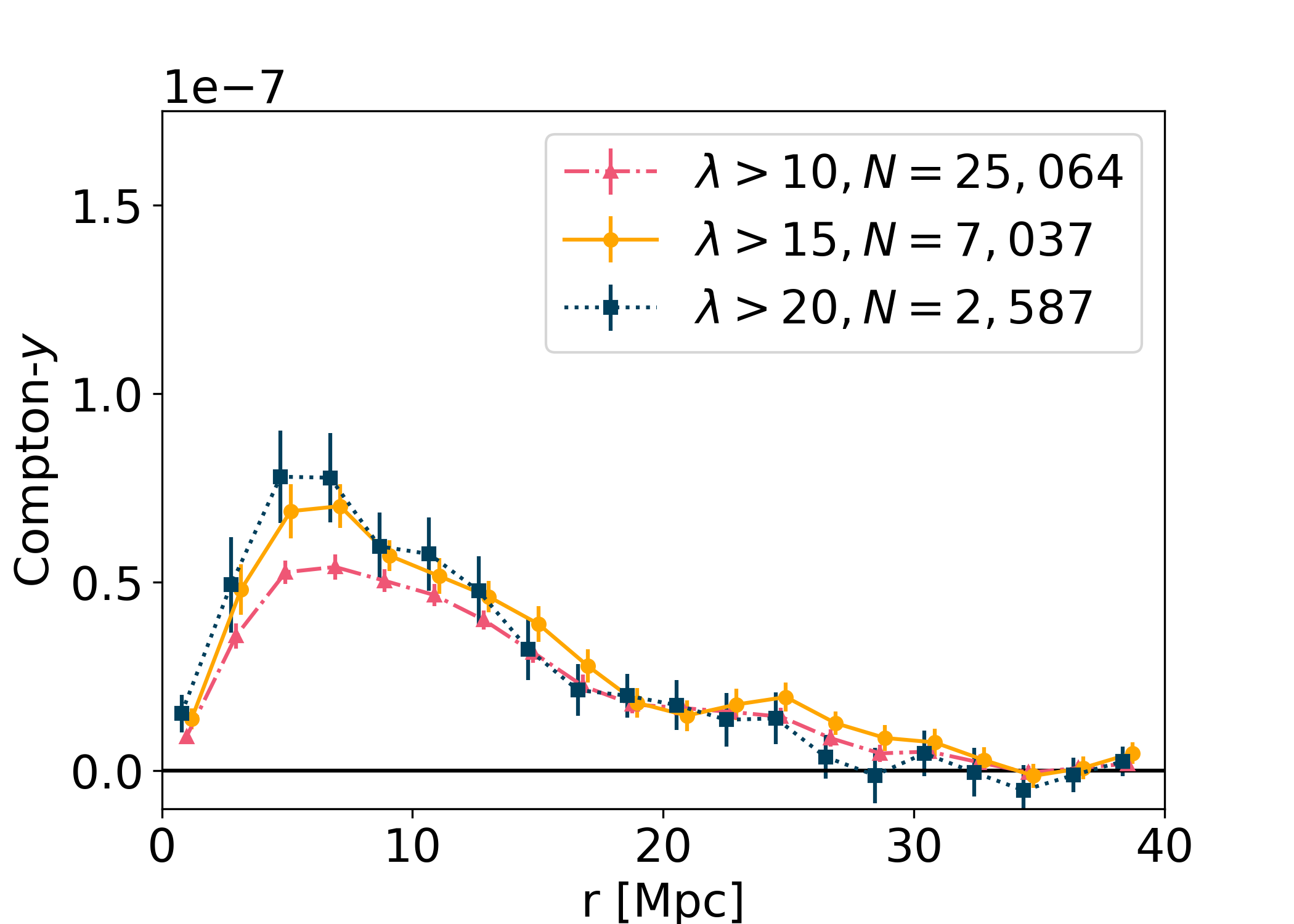 |
 |
 |
|
 |
 |
 |
V.2 Dependence on parameters
We examine the dependence of superclustering signal on cluster richness , field excursion , field ellipticity , and smoothing scale using the Buzzard mocks. Figure 15 shows the effects of imposing minimum limits on , , and on the stacked Compton- signal. The property has the strongest impact, demonstrating that clusters embedded in large-scale highly overdense regions tend to be members of more massive filaments and superclusters.

Certain cuts to the cluster sample significantly boost oriented signal, yet a reduction of factor to the number of stacked images augments the random noise by . For the different parameter values tested, we assess this trade-off by examining the signal-to-noise of the maximum bin of . We find that the full sample has the highest signal-to-noise. If including the field constraints, a combination of () is optimal.
Next we examine changes to the smoothing scale that is applied to the maps. As Figure 16 visually demonstrates, finer-grained smoothing causes the orientation for each cluster to be more dependent on local features such as nearby filament galaxies, whereas coarser smoothing makes larger-scale features (like the nearest-neighbor clusters) more important to the determination of curvature. With the Buzzard simulations, we perform oriented stacking with a Gaussian-smoothed map of FWHM=[6, 10, 14, 18] Mpc. The results are shown in Figure 18. We only show for brevity, but displays similar effects.


We find that the location of the peak of the profile scales nearly linearly with the smoothing scale. This is because the smoothing scale sets the radius from the cluster at which orientation is determined, and thus by construction, anisotropic structure is maximally aligned along the horizontal image axis of the stack at that radius. We will call this the ‘radius of maximal alignment.’ Figure 18 demonstrates this concept by rescaling the -axis by the Gaussian FWHM, bringing nearly all peaks into alignment. , not shown, behaves similarly. We emphasize that the peak location therefore contains little to no physical information. The height of the profile at the radius of maximal alignment, however, is physical, as it is determined by the average temperature and density of aligned structure at that scale. We will further analyse the meaning of peak height and its relationship to physical properties in a subsequent paper.
Another useful quantity is the total integrated Compton- signal for each moment,
| (13) |
where is defined in Equation 7. For , this is similar to the unitless angularly-integrated Compton- parameter, with the difference that our has units of Mpc2. is shown in the lower panel of Figure 18. depends not only on the gas properties at the radius of maximal alignment, but also on how coherent the structure is within and beyond that radius. It also depends on the galaxy field constraints and , which limit the cluster sample in a smoothing-dependent manner. As the smoothing becomes coarser, we observe that the profiles broaden and increases. This may suggest that LSS is more coherently aligned along the direction of orientation determined for larger scales than for smaller scales. However, because of the nontrivial impacts of smoothing on the galaxy field constraints, we leave a more robust physical interpretation for the succeeding paper.
The flexibility of our method to smoothing demonstrates that it can be applied to scales as small as individual clusters, to study the alignment of galaxies and cluster gas, and as large as the longest superclusters.
VI Comparison with Observational Data
We apply the method to ACTDES data and the Buzzard mocks using a few combinations of smoothing scales and field constraints. We will highlight results for 18 Mpc smoothing, a scale which roughly corresponds to inter-cluster filaments (as motivated in Sec. IV.2). We later show all three smoothing scales. Each result figure shows the observational measurements in 3 radial bins, as motivated in Sec IV.5. Each figure also shows the Buzzard results, which demonstrate what a ‘pure’ measurement would look like across the full DES footprint, with errorbars due to variance in the large scale structure but not instrumental noise. The Buzzard results are binned into the same 3 radial bins to assess the consistency with observations, while the figures also display the continuous Buzzard profiles for visual purposes.
To begin, we briefly examine the isotropic () component of the stacked images in Figure 19. This is identical for an oriented and unoriented stack and will not provide specific information about filaments. Nevertheless, comparing the Compton- signal beyond the stacked cluster radius between simulations and observations is informative of how well the simulations reproduce the large-scale clustering and gas content of halos.
Because our focus lies beyond the cluster interior, we exclude the majority of central-cluster tSZ contributions to the radial profile by choosing an inner cutoff radius. Our choice is , where is the redMaPPer cluster radius (Rykoff et al. 2014). is given by physical Mpc, which we calculate at the median richness in our sample, . After conversion, this results in a comoving radius of Mpc for the average redshift of the cluster sample. Therefore, in both the simulations and real data, we begin binning the signal beyond 2.5 Mpc.
The raw ACTDES profiles each have a constant positive offset with respect to the Buzzard profiles (not shown in any figure). This is primarily due to long-wavelength noise in the map from residual low- primary CMB contamination which does not average down with more stacked clusters. Stacks on random points in simulations of the ACT map described in Section IV.5 each result in a different constant offset depending on different realizations of the low- primary CMB. To account for the offset in the real ACT map and each simulation, we subtract the average value of from 33 to 40 Mpc (the tail of each profile) from the full profile. This is similar to performing aperture photometry, a technique typically applied to unoriented stacks to subtract the noise calculated in an annulus from the signal within some inner radius.

The adjusted profiles for 18 Mpc smoothing, after subtraction of the tail, are shown in Figure 19. There is a nonzero signal in the first two bins which is boosted when the constraint is applied. (The constraint has little to no effect on the isotropic profile, as previously demonstrated in Figure 15). The and constraints reduce the cluster sample by a factor of , causing an increase in noise of . We can determine the signal-to-noise of the results by comparing them to a null profile. This null result corresponds to the unphysical hypothesis that there is no tSZ signal outside of the average cluster radius. This would occur in a universe where every cluster were separated by Mpc from the nearest object containing hot gas. We compute the reduced- of the observational data vector (the coarsely binned profile) with respect to null:
| (14) |
where is the inverse covariance matrix of the data. Next, we find the probability that a truly null vector could exceed that . This Probability to Exceed (PTE) is measured by drawing 1 million random vectors from a normal distribution with mean zero and the covariance matrix from the data. We compute the of each vector with respect to null, then find the fraction of the sample for which the exceeds that of the real data vector. This fraction is the PTE; lower values indicate that the random vector is unlikely to exceed the true data vector, providing stronger evidence for a detection of non-zero signal in the data. We then relate this to a signal-to-noise (SNR) estimate which is the number of Gaussian sigmas away from null,
| (15) |
where erf is the error function. We also assess the goodness-of-fit to the Buzzard results by finding the reduced :
| (16) |
where is the summed covariance matrix for observational data and simulations, and refers to the coarsely binned Buzzard profile.
The bins are highly correlated for , so the SNR is only 1.7 and 2.3 for the profiles without and with constraints, respectively. Both profiles agree well with Buzzard, with . The low SNR of this extended isotropic signal, and the requirement to subtract a constant offset, are both arguments that extended structure is not probed well by unoriented stacking. Notably, the same constant offset does not appear in or . In addition, we achieve a higher-SNR detection with .
The moment of each stacked image, for the same 18 Mpc smoothing scale, is presented in Figure 20. We again remove the inner cluster region when coarsely binning the data to avoid cluster mis-centering effects. The binning is slightly uneven, designed to place the first bin at the location of the Buzzard continuous-profile peak. The signal for all clusters in Buzzard peaks at . Enforcing () raises the signal at the peak by a factor of . The Buzzard results are in strong agreement with ACTDES. We also show a null test, the of an ‘unoriented’ stack in which each cluster cutout was randomly rotated before stacking. This profile is consistent with zero as expected. Additionally, the figure shows the covariance matrices for both ACTDES data vectors.
We compare the signal to a completely null profile – corresponding to a perfectly isotropic stack – to determine its significance. Having no signal in would indicate that either (a) the average thermal energy distribution surrounding clusters is highly isotropic, (b) the galaxy distribution is uncorrelated with the gas distribution, or (c) our oriented stacking method does not effectively align large-scale structure. Table 3 presents the reduced-, PTE, and SNR values. Without constraints on the galaxy field, the ACTDES oriented stacks have 3.5 level evidence for signal in the moment. Introducing the field constraints does not change the significance, as the larger errorbars compensate for the boost in signal. Table 4 presents similar summary statistics for the Buzzard results, which have much higher significance (12 and 10) because of the lack of instrumental noise and larger cluster sample.
Finally, the results are shown in Figure 21. The same bins are applied to as . The Buzzard profiles peak at times smaller values than . For this component, a null profile could correspond to any of the (a), (b), and (c) possibilities listed for or the signal from a perfectly Gaussian random field. As shown in Tables 4 and 3, the Buzzard component from the constrained cluster sample is at , but the corresponding ACTDES result is only 1.5. Therefore, we can not claim evidence for the component in observations. The profiles are in agreement with Buzzard.


| m | Cuts (Y/N) | PTE | SNR | (d.o.f. = 3) | ||
|---|---|---|---|---|---|---|
| absolute | data-sim | |||||
| FWHM of smoothing = | ||||||
| 2 | Y | 1190 | 0.06 | 2.6 | 1.8 | 0.9 |
| 4 | Y | 1190 | 0.3 | 2.4 | 3.9 | 1.2 |
| FWHM of smoothing = | ||||||
| 2 | Y | 1103 | 0.004 | 3.2 | 5.2 | 0.5 |
| 4 | Y | 1103 | 0.2 | 1.5 | 1.8 | 1.1 |
| FWHM of smoothing = | ||||||
| 2 | N | 5494 | 0.0004 | 3.5 | 6.0 | 0.1 |
| 4 | N | 5494 | 0.4 | 0.9 | 1.0 | 0.2 |
| 2 | Y | 975 | 0.0005 | 3.5 | 5.9 | 0.07 |
| 4 | Y | 975 | 0.1 | 1.5 | 1.8 | 0.3 |
Note. — From left to right, is the multipole moment, ‘Cuts’ refers to whether or not the cluster sample has been constrained by ; is the number of stacked clusters, PTE is the probability to exceed, SNR gives the number of Gaussian from null, and is the reduced value using 3 degrees of freedom (d.o.f.). is shown for the absolute value with respect to 0 as well as the value with respect to Buzzard. The highest signal-to-noise detections of extended signal come from the components of the and smoothed stacks. Data and simulation are generally in agreement, with (data-sim) consistently near or below 1.
| m | Cuts (Y/N) | SNR | (d.o.f. = 3) | |
|---|---|---|---|---|
| FWHM of smoothing = | ||||
| 2 | Y | 6165 | 10 | 31 |
| 4 | Y | 6165 | 4.8 | 7.8 |
| FWHM of smoothing = | ||||
| 2 | Y | 5401 | 11 | 37 |
| 4 | Y | 5401 | 5.3 | 9.2 |
| FWHM of smoothing = | ||||
| 2 | N | 24,922 | 12 | 51 |
| 4 | N | 24,922 | 3.9 | 5.1 |
| 2 | Y | 4,836 | 9.5 | 30 |
| 4 | Y | 4,836 | 2.8 | 2.6 |
Note. — The table repeats the calculations in Table 3 for the Buzzard simulations, with the same 3 radial bins. is only shown for the ‘absolute’ value, as the (data-sim) value is already presented in Table 3. Because the simulation results are high-SNR, rather than calculating a PTE we simply estimate SNR by taking the square root of . Generally, the detection significance is much higher for Buzzard than for ACTDES because the simulation is noiseless. is detected at a much higher significance than .
We repeat the stacking procedure for two smaller smoothing scales, FWHM=10 Mpc and FWHM=14 Mpc, with the and contraints enforced for the respective smoothed maps. The plots are shown in Figure 22. The binning is adjusted for each scale to align the first bin with the peak location. The continuous profiles in the figures are shown for visual purposes but cannot be directly compared to the binned real data; instead, this comparison is best captured in the column of Table 3.
There is evidence for signal at the 3.2 level for 14 Mpc smoothing and marginal 2.6 evidence for 10 Mpc. The SNR of is smaller in all cases, although there is marginal for an component in the smallest smoothing scale. This is consistent with the expectation that non-Gaussianity is more pronounced on smaller scales. However, because the evidence does not meet the 3 threshold, we leave further analysis to future work with larger data sets. Generally, the observed data are in very good agreement with the simulations, reaching at most a reduced- of 1.2.
Due to the lack of detection in , we cannot claim to find evidence for non-Gaussian structure with the currently available data. For , as discussed in Section IV.6, the boost from applying the and thresholds only occurs in realistic fields and not in a Gaussian random field. Therefore, it is likely that the strength of in stacks on the constrained cluster sample is indicative of non-Gaussianity. However, to robustly address this, we would need to repeat the study in Section IV.6 with the exact methods applied to the final results (using thin redshift slicing, rescaling, and combining multiple slices). We leave this detailed comparison for future work.


As discussed in Section V.2, the shape of each profile is highly dependent on smoothing scale and thus the integrated profile provides a useful single-value quantity for comparison between data and simulations. Figure 23 shows the integrated signal (computed with a Riemann sum) over the Buzzard (red) and ACTDES (blue) coarsely-binned profiles for three smoothing scales. Errors are propagated with the covariance matrix for each scale. At all scales, the Buzzard and ACT integrals are within 1 of each other. The ACT integrals have SNR=[1.0, 2.0, 2.7] for the [10, 14, 18] Mpc smoothing scales. Therefore, we find marginal indications of integrated anisotropic clustering of thermal energy for the two coarser scales.

VII Conclusions
VII.1 Overview
This paper introduced a new real-space method for probing anisotropies in gas signal in the cosmic web. By combining millimeter-wavelength data from the ACT CMB survey with optical data from the DES galaxy survey, we measured the average superclustering signal from hot gas surrounding DES redMaPPer clusters. We showed that there is a significant Compton- signal from non-Gaussianity in the late-time universe visible in the moment of simulated stacks. There is a marginal indication for signal in the observational data. Using characteristics of the galaxy field, we identified highly overdense, elongated regions. Selecting for clusters in these high-superclustering areas enhances the gas signal in the moment of oriented stacks, causing a distinction from a Gaussian random field. We visually demonstrated this enhancement in the observational data, leaving a more rigorous proof of non-Gaussianity to future work. Generally, with observed ACTDES data, we found marginal-to-significant evidence for extended signal in the moments; the significance depended on the chosen galaxy field smoothing. This evidence demonstrates that the average thermal energy distribution around clusters is not isotropic. This, of course, is expected because clusters are embedded in filamentary structures in the cosmic web spanning a wide range of scales. Comparing to the Buzzard mocks showed broad agreement in the and radial profiles. For the integrated Compton- from , the results at all scales are in agreement.
We did not attempt to constrain the contribution of the WHIM, due to gas outside individual halos, to the anisotropic signal. In a previous filament-stacking study, de Graaff et al. 2019 found a filament signal with = . The team also found that bound gas in halos only contributes % of this signal. A WHIM signal at , then, is of the peak signal measured in our work. If the de Graaff et al. 2019 study was correct, this indicates that as expected, the dominant tSZ signal from the extended large-scale structure surrounding clusters comes from bound gas in halos. The previously-measured WHIM signal is smaller than any of the 1 error bars in our work and thus undetectable with the current method and data. A detection may be possible with the currently available data by stacking on all galaxies instead of clusters, as well as by applying a more sophisticated approach to the combination of smoothing scales and field constraints. A WHIM detection may also be possible with the future, expanded version of the ACT map and greater overlap with DES cluster data. We leave a detailed study of how oriented stacking can be used to characterize the WHIM for future work.
With the Websky full-sky simulations, we demonstrated the potential of the oriented stacking method to probe the evolution of superclustering out to and the relationship between cluster mass and the surrounding environment. These theory results demonstrated that the anisotropic gas signal from superclustering is expected to grow with time from to , then stabilize. For fixed redshift, the strength of superclustering correlates with cluster mass, indicating that massive clusters are embedded in more massive and/or denser filaments. The limited number of available clusters in the ACT map overlapping with DES prohibited the same analyses on real data.
VII.2 Systematics and Future Outlook
We identify a few sources of systematic uncertainty which were negligible in this study but will become important as the ACT data expands and improves in the next few years. First, as noted in Section II, redMaPPer clusters are known to contain false detections. False clusters should be less correlated with the surrounding large-scale structure than real clusters, and therefore their inclusion should bias our results low. Nevertheless, we found evidence for superclustering in ACTDES, indicating that the impact of cluster sample impurities was not enough to drown out the signal. Estimating how much higher the signal would be with a completely clean sample is beyond the scope of this work, as these low-richness impurities have not yet been well-characterized.
A possible source of systematic error in the comparison with simulations, as noted in Section II, is the failure of Buzzard to reproduce the redMaPPer mass-richness relation. As the errors on ACTDES decrease with future data, this may become a source of tension between the simulation and data. However, there are reasons to suspect this has a minor effect on our measurements compared to other factors such as the imperfect gas prescription applied to Buzzard. First, because this work does not focus on the cluster interior, discrepancies in the richness distribution are only important to the extent that they correlate with the surrounding large-scale structure. We found in section V.2 that cluster richness is indeed correlated with the anisotropic Compton- signal; however, this is subdominant compared to the dependence on evaluated at larger scales. Additionally, because the mock Compton- map is created using only halo information from the Buzzard dark-matter-only simulation, the map signal does not depend on the realistic identification of redMaPPer clusters. The most important steps in our pipeline are the selection and orientation of clusters using the redMaGiC mock galaxy data, where Buzzard does well in matching DES. It may be possible to entirely avoid the mass-richness systematic in future work by using the Buzzard state-of-the-art: a recent version of Buzzard improves the color-dependent clustering which heavily affects redMaPPer selection (DeRose et al. 2022). In general, to fully understand the factors influencing the oriented tSZ signal, we must disentangle the effects of cosmology, galaxy and cluster modelling/selection, and gas prescription. A succeeding paper will address this by applying oriented stacking to the galaxy distribution alone and comparing the DES results to Buzzard.
Moving forward, future Compton- maps from ACT will cover a sky area with complete overlap with DES over the 5000 sq. deg. footprint (Naess et al. 2020). They will additionally include high-resolution 30, 40, and 230 GHz data collected using Advanced ACT arrays, allowing for better removal of contamination from Galactic synchrotron sources, extragalactic radio sources, the cosmic infrared background, and dust (Madhavacheril et al. 2020). Our study will be repeated with the full cluster sample from DES, which is approximately 14 times larger than the sample used in this study. The systematic error contribution is at the few percent level for the current map, so random errors will still dominate. Therefore, the error bars on the data are expected to shrink by a factor of . If the binned values in the profile for 18 Mpc smoothing remained the same with 3.7 smaller error bars, the detection of signal after and cuts will be at the 13 level. The component would be detectable at the 5 level for the same scale. Slight tension would emerge with Buzzard, with a of 2.5. With the next iteration of ACT data, oriented stacking will be able to address questions of non-Gaussianity and assess the accuracy of the tSZ pasting prescriptions in simulations in more detail.
Additionally, the larger cluster sample will allow us to remove low- clusters and repeat the study with a more pure, higher-richness sample. This is expected to boost the superclustering gas signal. In a succeeding paper, we will use this expanded data to study the impact of the WHIM on the superclustering signal from hot gas.
Looking further to the future, The Simons Observatory (Ade et al. 2019, SO,) is currently being built in Chile, expected to begin taking CMB observations in the mid-2020s. With measurements in 6 frequencies, the SO Compton- map will attain lower noise levels and higher resolution than that of ACT. In addition, upcoming telescopes like the Fred Young Sub-millimeter Telescope (Terry et al. 2019, fomerly CCAT-p,) and the future CMB S4 mission (Carlstrom et al. 2019) will further advance tSZ measurements by mapping the millimeter sky with improved sensitivity and frequency coverage.
To optimize the science returns from oriented stacking, these higher quality CMB maps will need to be coupled with augmented cluster and galaxy data. The SO team predicts that the number of clusters detected through the tSZ effect will rise by an order of magnitude from current levels (Ade et al. 2019). The sample will extend to further redshifts than the DES red-sequence-detected sample because the tSZ effect is redshift-independent, whereas received flux from optical galaxy observations (as in DES) diminishes with redshift. SO forecasts detected clusters in a bin of width at , whereas the DES RedMaPPer catalog extends only to . Higher-redshift clusters will enable us to measure the evolution of superclustering further into the universe’s past. In addition, the Dark Energy Spectroscopic Instrument (Dey et al. 2019, DESI,) will provide many new spectroscopic redshifts for galaxies and clusters, enabling improved tomographic slicing to study redshift evolution of the LSS (Zou et al. 2021). The Vera C. Rubin Observatory Legacy Survey of Space and Time (Ivezić et al. 2019, LSST,) will make unprecedented contributions to the optical galaxy and cluster data with deep observations of the Southern sky resulting in an estimated 20 billion galaxies. Looking to other wavelengths, eROSITA is expected to deliver hundreds of superclusters detected in the X-ray: additional objects on which to stack the tSZ signal (Ghirardini et al. 2021). Applying the methods detailed in this paper to combinations of these varied data sets, where they overlap, will greatly increase the signal-to-noise and redshift extent of superclustering measurements.
This paper demonstrates a flexible tool for examining superclustering in the universe. We have shown its effectiveness for a combination of galaxy and gas data, but it can also be used to combine galaxy and weak lensing data or to probe the anisotropies of the galaxy field alone. By combining different probes, this method can be implemented to study the anisotropic bias of galaxies and gas with respect to dark matter. A follow-up paper will use oriented stacking on galaxy number density maps and compare the results to extended gas signal to probe information about the anisotropic bias, the baryonic content of halos, and possibly the baryons outside of halos. This may provide more insight into the census of baryonic content in filaments. In addition, future work will determine whether this method of measuring anisotropic clustering can complement two-point clustering statistics in constraining viable models of dark energy.
Acknowledgments
We thank the anonymous referee for providing valuable comments which improved the quality of this paper.
Canadian co-authors acknowledge support from the Natural Sciences and Engineering Research Council of Canada. Computations were performed on the SciNet supercomputer at the SciNet HPC Consortium. SciNet is funded by: the Canada Foundation for Innovation; the Government of Ontario; Ontario Research Fund - Research Excellence; and the University of Toronto.
The authors thank Bruce Partridge for useful and extensive comments on the draft.
JRB’s research was funded by the Natural Sciences and Engineering Research Council of Canada Discovery Grant Program and a fellowship from the Canadian Institute for Advanced Research (CIFAR) Gravity and Extreme Universe program.
ADH acknowledges support from the Sutton Family Chair in Science, Christianity and Cultures.
R. H. is a CIFAR Azrieli Global Scholar, Gravity & the Extreme Universe Program, 2019, and a 2020 Alfred P. Sloan Research Fellowship. RH is supported by Natural Sciences and Engineering Research Council of Canada Discovery Grant Program and the Connaught Fund.
JPH acknowledges funding for SZ cluster studies from NSF AAG number AST-1615657.
KM acknowledges support from the National Research Foundation of South Africa.
This work was supported by the U.S. National Science Foundation through awards AST-0408698, AST-0965625, and AST-1440226 for the ACT project, as well as awards PHY-0355328, PHY-0855887 and PHY-1214379. Funding was also provided by Princeton University, the University of Pennsylvania, and a Canada Foundation for Innovation (CFI) award to UBC. ACT operates in the Parque Astronómico Atacama in northern Chile under the auspices of the Comisión Nacional de Investigación (CONICYT). The development of multichroic detectors and lenses was supported by NASA grants NNX13AE56G and NNX14AB58G. Detector research at NIST was supported by the NIST Innovations in Measurement Science program.
Funding for the DES Projects has been provided by the U.S. Department of Energy, the U.S. National Science Foundation, the Ministry of Science and Education of Spain, the Science and Technology Facilities Council of the United Kingdom, the Higher Education Funding Council for England, the National Center for Supercomputing Applications at the University of Illinois at Urbana-Champaign, the Kavli Institute of Cosmological Physics at the University of Chicago, the Center for Cosmology and Astro-Particle Physics at the Ohio State University, the Mitchell Institute for Fundamental Physics and Astronomy at Texas A&M University, Financiadora de Estudos e Projetos, Fundação Carlos Chagas Filho de Amparo à Pesquisa do Estado do Rio de Janeiro, Conselho Nacional de Desenvolvimento Científico e Tecnológico and the Ministério da Ciência, Tecnologia e Inovação, the Deutsche Forschungsgemeinschaft and the Collaborating Institutions in the Dark Energy Survey.
The Collaborating Institutions are Argonne National Laboratory, the University of California at Santa Cruz, the University of Cambridge, Centro de Investigaciones Energéticas, Medioambientales y Tecnológicas-Madrid, the University of Chicago, University College London, the DES-Brazil Consortium, the University of Edinburgh, the Eidgenössische Technische Hochschule (ETH) Zürich, Fermi National Accelerator Laboratory, the University of Illinois at Urbana-Champaign, the Institut de Ciències de l’Espai (IEEC/CSIC), the Institut de Física d’Altes Energies, Lawrence Berkeley National Laboratory, the Ludwig-Maximilians Universität München and the associated Excellence Cluster Universe, the University of Michigan, NFS’s NOIRLab, the University of Nottingham, The Ohio State University, the University of Pennsylvania, the University of Portsmouth, SLAC National Accelerator Laboratory, Stanford University, the University of Sussex, Texas A&M University, and the OzDES Membership Consortium.
Based in part on observations at Cerro Tololo Inter-American Observatory at NSF’s NOIRLab (NOIRLab Prop. ID 2012B-0001; PI: J. Frieman), which is managed by the Association of Universities for Research in Astronomy (AURA) under a cooperative agreement with the National Science Foundation.
The DES data management system is supported by the National Science Foundation under Grant Numbers AST-1138766 and AST-1536171. The DES participants from Spanish institutions are partially supported by MICINN under grants ESP2017-89838, PGC2018-094773, PGC2018-102021, SEV-2016-0588, SEV-2016-0597, and MDM-2015-0509, some of which include ERDF funds from the European Union. IFAE is partially funded by the CERCA program of the Generalitat de Catalunya. Research leading to these results has received funding from the European Research Council under the European Union’s Seventh Framework Program (FP7/2007-2013) including ERC grant agreements 240672, 291329, and 306478. We acknowledge support from the Brazilian Instituto Nacional de Ciência e Tecnologia (INCT) do e-Universo (CNPq grant 465376/2014-2).
This manuscript has been authored by Fermi Research Alliance, LLC under Contract No. DE-AC02-07CH11359 with the U.S. Department of Energy, Office of Science, Office of High Energy Physics.
This work received support from the U.S. Department of Energy under contract number DE-AC02-76SF00515 at SLAC National Accelerator Laboratory. This research used computing resources at SLAC National Accelerator Laboratory and at the National Energy Research Scientific Computing Center (NERSC), a U.S. Department of Energy Office of Science User Facility located at Lawrence Berkeley National Laboratory, operated under Contract No. DE-AC02-05CH11231.
References
- Abbott et al. (2020) Abbott, T. M. C., Aguena, M., Alarcon, A., et al. 2020, Phys. Rev. D, 102, 023509, doi: 10.1103/PhysRevD.102.023509
- Ade et al. (2019) Ade, P., Aguirre, J., Ahmed, Z., et al. 2019, J. Cosmology Astropart. Phys, 2019, 056, doi: 10.1088/1475-7516/2019/02/056
- Aiola et al. (2020) Aiola, S., Calabrese, E., Maurin, L., et al. 2020, J. Cosmology Astropart. Phys, 2020, 047, doi: 10.1088/1475-7516/2020/12/047
- Alam et al. (2017) Alam, S., Ata, M., Bailey, S., et al. 2017, MNRAS, 470, 2617, doi: 10.1093/mnras/stx721
- Amodeo et al. (2021) Amodeo, S., Battaglia, N., Schaan, E., et al. 2021, Phys. Rev. D, 103, 063514, doi: 10.1103/PhysRevD.103.063514
- Aragón-Calvo et al. (2010) Aragón-Calvo, M. A., van de Weygaert, R., & Jones, B. J. T. 2010, MNRAS, 408, 2163, doi: 10.1111/j.1365-2966.2010.17263.x
- Astropy Collaboration et al. (2013) Astropy Collaboration, Robitaille, T. P., Tollerud, E. J., et al. 2013, A&A, 558, A33, doi: 10.1051/0004-6361/201322068
- Astropy Collaboration et al. (2018) Astropy Collaboration, Price-Whelan, A. M., Sipőcz, B. M., et al. 2018, AJ, 156, 123, doi: 10.3847/1538-3881/aabc4f
- Bagchi et al. (2017) Bagchi, J., Sankhyayan, S., Sarkar, P., et al. 2017, ApJ, 844, 25, doi: 10.3847/1538-4357/aa7949
- Bardeen et al. (1986) Bardeen, J. M., Bond, J. R., Kaiser, N., & Szalay, A. S. 1986, ApJ, 304, 15, doi: 10.1086/164143
- Basilakos et al. (2001) Basilakos, S., Plionis, M., & Rowan-Robinson, M. 2001, MNRAS, 323, 47, doi: 10.1046/j.1365-8711.2001.04226.x
- Battaglia et al. (2012a) Battaglia, N., Bond, J. R., Pfrommer, C., & Sievers, J. L. 2012a, ApJ, 758, 74, doi: 10.1088/0004-637X/758/2/74
- Battaglia et al. (2012b) —. 2012b, ApJ, 758, 75, doi: 10.1088/0004-637X/758/2/75
- Battaglia et al. (2010) Battaglia, N., Bond, J. R., Pfrommer, C., Sievers, J. L., & Sijacki, D. 2010, ApJ, 725, 91, doi: 10.1088/0004-637X/725/1/91
- Bharadwaj & Pandey (2004) Bharadwaj, S., & Pandey, B. 2004, ApJ, 615, 1, doi: 10.1086/424476
- Bond & Efstathiou (1987) Bond, J. R., & Efstathiou, G. 1987, MNRAS, 226, 655, doi: 10.1093/mnras/226.3.655
- Bond et al. (1996) Bond, J. R., Kofman, L., & Pogosyan, D. 1996, Nature, 380, 603, doi: 10.1038/380603a0
- Bond & Myers (1996) Bond, J. R., & Myers, S. T. 1996, ApJS, 103, 1, doi: 10.1086/192267
- Borgani (1995) Borgani, S. 1995, Phys. Rep., 251, 1, doi: 10.1016/0370-1573(94)00073-C
- Bouma et al. (2021) Bouma, S. J. D., Richter, P., & Wendt, M. 2021, A&A, 647, A166, doi: 10.1051/0004-6361/202039786
- Carlstrom et al. (2019) Carlstrom, J., Abazajian, K., Addison, G., et al. 2019, in Bulletin of the American Astronomical Society, Vol. 51, 209. https://arxiv.org/abs/1908.01062
- Carlstrom et al. (2002) Carlstrom, J. E., Holder, G. P., & Reese, E. D. 2002, ARA&A, 40, 643, doi: 10.1146/annurev.astro.40.060401.093803
- Cen (1994) Cen, R. 1994, ApJ, 424, 22, doi: 10.1086/173868
- Cen & Ostriker (1999) Cen, R., & Ostriker, J. P. 1999, ApJ, 514, 1, doi: 10.1086/306949
- Cen & Ostriker (2006) —. 2006, ApJ, 650, 560, doi: 10.1086/506505
- Choi et al. (2018) Choi, S. K., Austermann, J., Beall, J. A., et al. 2018, Journal of Low Temperature Physics, 193, 267, doi: 10.1007/s10909-018-1982-4
- Clampitt et al. (2017) Clampitt, J., Sánchez, C., Kwan, J., et al. 2017, MNRAS, 465, 4204, doi: 10.1093/mnras/stw2988
- Codis et al. (2018a) Codis, S., Jindal, A., Chisari, N. E., et al. 2018a, MNRAS, 481, 4753, doi: 10.1093/mnras/sty2567
- Codis et al. (2018b) Codis, S., Pogosyan, D., & Pichon, C. 2018b, MNRAS, 479, 973, doi: 10.1093/mnras/sty1643
- Coil (2013) Coil, A. L. 2013, in Planets, Stars and Stellar Systems. Volume 6: Extragalactic Astronomy and Cosmology, ed. T. D. Oswalt & W. C. Keel, Vol. 6 (Dordrecht:Springer), 387, doi: 10.1007/978-94-007-5609-0_8
- Costanzi et al. (2021) Costanzi, M., Saro, A., Bocquet, S., et al. 2021, Phys. Rev. D, 103, 043522, doi: 10.1103/PhysRevD.103.043522
- Darragh Ford et al. (2019) Darragh Ford, E., Laigle, C., Gozaliasl, G., et al. 2019, MNRAS, 489, 5695, doi: 10.1093/mnras/stz2490
- Dawson et al. (2013) Dawson, K. S., Schlegel, D. J., Ahn, C. P., et al. 2013, AJ, 145, 10, doi: 10.1088/0004-6256/145/1/10
- de Graaff et al. (2019) de Graaff, A., Cai, Y.-C., Heymans, C., & Peacock, J. A. 2019, A&A, 624, A48, doi: 10.1051/0004-6361/201935159
- DeRose et al. (2019) DeRose, J., Wechsler, R. H., Becker, M. R., et al. 2019, arXiv e-prints, arXiv:1901.02401. https://arxiv.org/abs/1901.02401
- DeRose et al. (2022) —. 2022, Phys. Rev. D, 105, 123520, doi: 10.1103/PhysRevD.105.123520
- Desjacques et al. (2018) Desjacques, V., Jeong, D., & Schmidt, F. 2018, Phys. Rep., 733, 1, doi: 10.1016/j.physrep.2017.12.002
- Dey et al. (2019) Dey, A., Schlegel, D. J., Lang, D., et al. 2019, AJ, 157, 168, doi: 10.3847/1538-3881/ab089d
- Einasto et al. (1997) Einasto, M., Tago, E., Jaaniste, J., Einasto, J., & Andernach, H. 1997, A&AS, 123, 119, doi: 10.1051/aas:1997340
- Flaugher et al. (2015) Flaugher, B., Diehl, H. T., Honscheid, K., et al. 2015, AJ, 150, 150, doi: 10.1088/0004-6256/150/5/150
- Fowler et al. (2007) Fowler, J. W., Niemack, M. D., Dicker, S. R., et al. 2007, Appl. Opt., 46, 3444, doi: 10.1364/AO.46.003444
- Frisch et al. (1995) Frisch, P., Einasto, J., Einasto, M., et al. 1995, A&A, 296, 611. https://arxiv.org/abs/astro-ph/9503037
- Ghirardini et al. (2021) Ghirardini, V., Bulbul, E., Hoang, D. N., et al. 2021, A&A, 647, A4, doi: 10.1051/0004-6361/202039554
- Giannantonio et al. (2012) Giannantonio, T., Porciani, C., Carron, J., Amara, A., & Pillepich, A. 2012, MNRAS, 422, 2854, doi: 10.1111/j.1365-2966.2012.20604.x
- Giodini et al. (2013) Giodini, S., Lovisari, L., Pointecouteau, E., et al. 2013, Space Sci. Rev., 177, 247, doi: 10.1007/s11214-013-9994-5
- Gitti et al. (2012) Gitti, M., Brighenti, F., & McNamara, B. R. 2012, Advances in Astronomy, 2012, 950641, doi: 10.1155/2012/950641
- Górski et al. (2005) Górski, K. M., Hivon, E., Banday, A. J., et al. 2005, ApJ, 622, 759, doi: 10.1086/427976
- Hand et al. (2011) Hand, N., Appel, J. W., Battaglia, N., et al. 2011, ApJ, 736, 39, doi: 10.1088/0004-637X/736/1/39
- Harris et al. (2020) Harris, C. R., Millman, K. J., van der Walt, S. J., et al. 2020, Nature, 585, 357, doi: 10.1038/s41586-020-2649-2
- Henderson et al. (2016) Henderson, S. W., Allison, R., Austermann, J., et al. 2016, Journal of Low Temperature Physics, 184, 772, doi: 10.1007/s10909-016-1575-z
- Hill et al. (2018) Hill, J. C., Baxter, E. J., Lidz, A., Greco, J. P., & Jain, B. 2018, Phys. Rev. D, 97, 083501, doi: 10.1103/PhysRevD.97.083501
- Ho et al. (2018) Ho, A., Gronke, M., Falck, B., & Mota, D. F. 2018, A&A, 619, A122, doi: 10.1051/0004-6361/201833899
- Ho et al. (2017) Ho, S.-P. P., Austermann, J., Beall, J. A., et al. 2017, in Millimeter, Submillimeter, and Far-Infrared Detectors and Instrumentation for Astronomy VIII, ed. W. S. Holland & J. Zmuidzinas, Vol. 9914, International Society for Optics and Photonics (SPIE), 301 – 315. https://doi.org/10.1117/12.2233113
- Hopkins et al. (2005) Hopkins, P. F., Bahcall, N. A., & Bode, P. 2005, ApJ, 618, 1, doi: 10.1086/425993
- Huang (2016) Huang, Z. 2016, Phys. Rev. D, 93, 043538, doi: 10.1103/PhysRevD.93.043538
- Ivezić et al. (2019) Ivezić, Ž., Kahn, S. M., Tyson, J. A., et al. 2019, ApJ, 873, 111, doi: 10.3847/1538-4357/ab042c
- Kolokotronis et al. (2002) Kolokotronis, V., Basilakos, S., & Plionis, M. 2002, MNRAS, 331, 1020, doi: 10.1046/j.1365-8711.2002.05263.x
- Kotecha et al. (2022) Kotecha, S., Welker, C., Zhou, Z., et al. 2022, MNRAS, 512, 926, doi: 10.1093/mnras/stac300
- Kraljic et al. (2020) Kraljic, K., Pichon, C., Codis, S., et al. 2020, MNRAS, 491, 4294, doi: 10.1093/mnras/stz3319
- Kravtsov et al. (2004) Kravtsov, A. V., Berlind, A. A., Wechsler, R. H., et al. 2004, ApJ, 609, 35, doi: 10.1086/420959
- Krolewski et al. (2019) Krolewski, A., Ho, S., Chen, Y.-C., et al. 2019, ApJ, 876, 52, doi: 10.3847/1538-4357/ab1010
- Kuchner et al. (2022) Kuchner, U., Haggar, R., Aragón-Salamanca, A., et al. 2022, MNRAS, 510, 581, doi: 10.1093/mnras/stab3419
- Li et al. (2018) Li, Y., Austermann, J. E., Beall, J. A., et al. 2018, in Society of Photo-Optical Instrumentation Engineers (SPIE) Conference Series, Vol. 10708, Millimeter, Submillimeter, and Far-Infrared Detectors and Instrumentation for Astronomy IX, ed. J. Zmuidzinas & J.-R. Gao, 107080A, doi: 10.1117/12.2313942
- Libeskind et al. (2018) Libeskind, N. I., van de Weygaert, R., Cautun, M., et al. 2018, MNRAS, 473, 1195, doi: 10.1093/mnras/stx1976
- Lim et al. (2018) Lim, S. H., Mo, H. J., Li, R., et al. 2018, ApJ, 854, 181, doi: 10.3847/1538-4357/aaaa21
- Louis et al. (2017) Louis, T., Grace, E., Hasselfield, M., et al. 2017, J. Cosmology Astropart. Phys, 2017, 031, doi: 10.1088/1475-7516/2017/06/031
- Madhavacheril et al. (2020) Madhavacheril, M. S., Hill, J. C., Næss, S., et al. 2020, Phys. Rev. D, 102, 023534, doi: 10.1103/PhysRevD.102.023534
- Maraston et al. (2013) Maraston, C., Pforr, J., Henriques, B. M., et al. 2013, MNRAS, 435, 2764, doi: 10.1093/mnras/stt1424
- McCarthy et al. (2003) McCarthy, I. G., Babul, A., Holder, G. P., & Balogh, M. L. 2003, ApJ, 591, 515, doi: 10.1086/375486
- McClintock et al. (2019) McClintock, T., Varga, T. N., Gruen, D., et al. 2019, MNRAS, 482, 1352, doi: 10.1093/mnras/sty2711
- Miller & LAMBDA group (2018) Miller, N., & LAMBDA group. 2018, in American Astronomical Society Meeting Abstracts, Vol. 231, American Astronomical Society Meeting Abstracts #231, 430.05
- Mroczkowski et al. (2019) Mroczkowski, T., Nagai, D., Basu, K., et al. 2019, Space Sci. Rev., 215, 17, doi: 10.1007/s11214-019-0581-2
- Naess et al. (2020) Naess, S., Aiola, S., Austermann, J. E., et al. 2020, J. Cosmology Astropart. Phys, 2020, 046, doi: 10.1088/1475-7516/2020/12/046
- Oort (1983) Oort, J. H. 1983, ARA&A, 21, 373, doi: 10.1146/annurev.aa.21.090183.002105
- Pandey et al. (2021) Pandey, S., Krause, E., DeRose, J., et al. 2021, arXiv e-prints, arXiv:2105.13545. https://arxiv.org/abs/2105.13545
- Peebles (1980) Peebles, P. J. E. 1980, The large-scale structure of the universe (Princeton University Press)
- Pessa et al. (2018) Pessa, I., Tejos, N., Barrientos, L. F., et al. 2018, MNRAS, 477, 2991, doi: 10.1093/mnras/sty723
- Plagge et al. (2010) Plagge, T., Benson, B. A., Ade, P. A. R., et al. 2010, ApJ, 716, 1118, doi: 10.1088/0004-637X/716/2/1118
- Planck Collaboration et al. (2013) Planck Collaboration, Ade, P. A. R., Aghanim, N., et al. 2013, A&A, 550, A131, doi: 10.1051/0004-6361/201220040
- Planck Collaboration et al. (2016a) Planck Collaboration, Aghanim, N., Arnaud, M., et al. 2016a, A&A, 594, A22, doi: 10.1051/0004-6361/201525826
- Planck Collaboration et al. (2016b) Planck Collaboration, Ade, P. A. R., Aghanim, N., et al. 2016b, A&A, 594, A16, doi: 10.1051/0004-6361/201526681
- Planck Collaboration et al. (2016c) —. 2016c, A&A, 594, A13, doi: 10.1051/0004-6361/201525830
- Puchwein et al. (2008) Puchwein, E., Sijacki, D., & Springel, V. 2008, ApJ, 687, L53, doi: 10.1086/593352
- Regaldo-Saint Blancard et al. (2021) Regaldo-Saint Blancard, B., Codis, S., Bond, J. R., & Stein, G. 2021, MNRAS, 504, 1694, doi: 10.1093/mnras/stab927
- Remazeilles et al. (2011) Remazeilles, M., Delabrouille, J., & Cardoso, J.-F. 2011, MNRAS, 410, 2481, doi: 10.1111/j.1365-2966.2010.17624.x
- Rozo et al. (2016) Rozo, E., Rykoff, E. S., Abate, A., et al. 2016, MNRAS, 461, 1431, doi: 10.1093/mnras/stw1281
- Rykoff et al. (2014) Rykoff, E. S., Rozo, E., Busha, M. T., et al. 2014, ApJ, 785, 104, doi: 10.1088/0004-637X/785/2/104
- Rykoff et al. (2016) Rykoff, E. S., Rozo, E., Hollowood, D., et al. 2016, ApJS, 224, 1, doi: 10.3847/0067-0049/224/1/1
- Santiago-Bautista et al. (2020) Santiago-Bautista, I., Caretta, C. A., Bravo-Alfaro, H., Pointecouteau, E., & Andernach, H. 2020, A&A, 637, A31, doi: 10.1051/0004-6361/201936397
- Schaan et al. (2021) Schaan, E., Ferraro, S., Amodeo, S., et al. 2021, Phys. Rev. D, 103, 063513, doi: 10.1103/PhysRevD.103.063513
- Sefusatti et al. (2006) Sefusatti, E., Crocce, M., Pueblas, S., & Scoccimarro, R. 2006, Phys. Rev. D, 74, 023522, doi: 10.1103/PhysRevD.74.023522
- Sehgal et al. (2010) Sehgal, N., Bode, P., Das, S., et al. 2010, ApJ, 709, 920, doi: 10.1088/0004-637X/709/2/920
- Sehgal et al. (2011) Sehgal, N., Trac, H., Acquaviva, V., et al. 2011, ApJ, 732, 44, doi: 10.1088/0004-637X/732/1/44
- Sehgal et al. (2013) Sehgal, N., Addison, G., Battaglia, N., et al. 2013, ApJ, 767, 38, doi: 10.1088/0004-637X/767/1/38
- Sevilla-Noarbe et al. (2021) Sevilla-Noarbe, I., Bechtol, K., Carrasco Kind, M., et al. 2021, ApJS, 254, 24, doi: 10.3847/1538-4365/abeb66
- Shull et al. (2012) Shull, J. M., Smith, B. D., & Danforth, C. W. 2012, ApJ, 759, 23, doi: 10.1088/0004-637X/759/1/23
- Sijacki et al. (2008) Sijacki, D., Pfrommer, C., Springel, V., & Enßlin, T. A. 2008, MNRAS, 387, 1403, doi: 10.1111/j.1365-2966.2008.13310.x
- Sijacki et al. (2007) Sijacki, D., Springel, V., Di Matteo, T., & Hernquist, L. 2007, MNRAS, 380, 877, doi: 10.1111/j.1365-2966.2007.12153.x
- Sonnenfeld et al. (2019) Sonnenfeld, A., Wang, W., & Bahcall, N. 2019, A&A, 622, A30, doi: 10.1051/0004-6361/201834260
- Springel et al. (2018) Springel, V., Pakmor, R., Pillepich, A., et al. 2018, MNRAS, 475, 676, doi: 10.1093/mnras/stx3304
- Stein et al. (2019) Stein, G., Alvarez, M. A., & Bond, J. R. 2019, MNRAS, 483, 2236, doi: 10.1093/mnras/sty3226
- Stein et al. (2020) Stein, G., Alvarez, M. A., Bond, J. R., van Engelen, A., & Battaglia, N. 2020, J. Cosmology Astropart. Phys, 2020, 012, doi: 10.1088/1475-7516/2020/10/012
- Sunyaev & Zeldovich (1970) Sunyaev, R. A., & Zeldovich, Y. B. 1970, Comments on Astrophysics and Space Physics, 2, 66
- Sunyaev & Zeldovich (1972) —. 1972, Comments on Astrophysics and Space Physics, 4, 173
- Swetz et al. (2011) Swetz, D. S., Ade, P. A. R., Amiri, M., et al. 2011, ApJS, 194, 41, doi: 10.1088/0067-0049/194/2/41
- Takada & Jain (2004) Takada, M., & Jain, B. 2004, MNRAS, 348, 897, doi: 10.1111/j.1365-2966.2004.07410.x
- Tanimura et al. (2020) Tanimura, H., Aghanim, N., Bonjean, V., Malavasi, N., & Douspis, M. 2020, A&A, 637, A41, doi: 10.1051/0004-6361/201937158
- Tanimura et al. (2019) Tanimura, H., Hinshaw, G., McCarthy, I. G., et al. 2019, MNRAS, 483, 223, doi: 10.1093/mnras/sty3118
- Tejos et al. (2016) Tejos, N., Prochaska, J. X., Crighton, N. H. M., et al. 2016, MNRAS, 455, 2662, doi: 10.1093/mnras/stv2376
- Terry et al. (2019) Terry, H., Battaglia, N., Basu, K., et al. 2019, in Bulletin of the American Astronomical Society, Vol. 51, 213. https://arxiv.org/abs/1909.02587
- The Dark Energy Survey Collaboration (2005) The Dark Energy Survey Collaboration. 2005, arXiv e-prints, astro. https://arxiv.org/abs/astro-ph/0510346
- Thornton et al. (2016) Thornton, R. J., Ade, P. A. R., Aiola, S., et al. 2016, ApJS, 227, 21, doi: 10.3847/1538-4365/227/2/21
- To et al. (2021) To, C., Krause, E., Rozo, E., et al. 2021, Phys. Rev. Lett., 126, 141301, doi: 10.1103/PhysRevLett.126.141301
- Tumlinson et al. (2017) Tumlinson, J., Peeples, M. S., & Werk, J. K. 2017, ARA&A, 55, 389, doi: 10.1146/annurev-astro-091916-055240
- van de Weygaert & Bond (2008a) van de Weygaert, R., & Bond, J. R. 2008a, in A Pan-Chromatic View of Clusters of Galaxies and the Large-Scale Structure, ed. M. Plionis, O. López-Cruz, & D. Hughes, Vol. 740 (Dordrecht: Springer), 24, doi: 10.1007/978-1-4020-6941-3_11
- van de Weygaert & Bond (2008b) —. 2008b, in A Pan-Chromatic View of Clusters of Galaxies and the Large-Scale Structure, ed. M. Plionis, O. López-Cruz, & D. Hughes, Vol. 740 (Dordrecht: Springer), 335, doi: 10.1007/978-1-4020-6941-3_10
- Wechsler et al. (2022) Wechsler, R. H., DeRose, J., Busha, M. T., et al. 2022, ApJ, 931, 145, doi: 10.3847/1538-4357/ac5b0a
- Welker et al. (2020) Welker, C., Bland-Hawthorn, J., Van de Sande, J., et al. 2020, MNRAS, 491, 2864, doi: 10.1093/mnras/stz2860
- Yang et al. (2020) Yang, T., Hudson, M. J., & Afshordi, N. 2020, MNRAS, 498, 3158, doi: 10.1093/mnras/staa2547
- Zel’Dovich (1970) Zel’Dovich, Y. B. 1970, A&A, 500, 13
- Zeldovich & Sunyaev (1969) Zeldovich, Y. B., & Sunyaev, R. A. 1969, Ap&SS, 4, 301, doi: 10.1007/BF00661821
- Zhang et al. (2019) Zhang, Y., Jeltema, T., Hollowood, D. L., et al. 2019, MNRAS, 487, 2578, doi: 10.1093/mnras/stz1361
- Zonca et al. (2019) Zonca, A., Singer, L., Lenz, D., et al. 2019, Journal of Open Source Software, 4, 1298, doi: 10.21105/joss.01298
- Zou et al. (2021) Zou, H., Gao, J., Xu, X., et al. 2021, ApJS, 253, 56, doi: 10.3847/1538-4365/abe5b0