3D MHD astrospheres: applications to IRC-10414 and Betelgeuse
Abstract
A significative fraction of all massive stars in the Milky Way move supersonically through their local interstellar medium (ISM), producing bow shock nebulae by wind-ISM interaction. The stability of these observed astrospheres around cool massive stars challenges precedent two-dimensional (magneto-)hydrodynamical simulations of their surroundings. We present three-dimensional magneto-hydrodynamical (3D MHD) simulations of the circumstellar medium of runaway M-type red supergiant stars moving with velocity . We treat the stellar wind with a Parker spiral and assume a magnetisation of the ISM. Our free parameter is the angle between ISM flow and magnetisation, taken to , and . It is found that simulation dimension, coordinate systems and grid effects can greatly affect the development of the modelled astrospheres. Nevertheless, as soon as the ISM flow and magnetisation directions differs by more than a few degrees (), the bow shock is stabilised, most clumpiness and ragged structures vanishing. The complex shape of the bow shocks induce important projection effects, e.g. at optical H line, producing complex of astrospheric morphologies. We speculate that those effects are also at work around earlier-type massive stars, which would explain their diversity of their observed arc-like nebula around runaway OB stars. Our 3D MHD models are fitting well observations of the astrospheres of several runaway red supergiant stars. The results interpret the smoothed astrosphere of IRC-10414 and Betelgeuse (Ori) are stabilised by an organised, non-parallel ambient magnetic field. Our findings suggest that IRC-10414 is currently in a steady state of its evolution, and that Betelgeuse’s bar is of interstellar origin.
Keywords:
methods: MHD – radiative transfer – stars: massive – stars: circumstellar matter.1 Introduction
Massive stars () are preponderant engines in the cycle of matter of the interstellar medium (ISM) of galaxies (Maeder 2009). They blow strong stellar winds, and, by synthetizing heavy chemical elements in their interiors, massive stars typically evolve from a long, hot, main-sequence phase to a short, cold red supergiant phase (Ekström et al. 2012). They may also experience series of eruptive, luminous blue mass-losing events and/or finally finish their lives as hot Wolf-Rayet stars, respectively (Vink 2006). The number, duration and stellar surface properties of these successive evolutionary phases are mostly determined by their initial mass, rotation rate (Brott et al. 2011; Szécsi et al. 2020), but also chemical composition (Sander et al. 2020), which uniquely characterise the evolution and fate of massive stars (Woosley et al. 2002). Throughout their lives, they lose mass and radiate strong ionizing photons, which both shape their surroundings as circumstellar bubble nebulae made of stellar wind and ISM material (Weaver et al. 1977).
The internal structures of wind-blown bubbles reflect the past stellar evolution of massive stars (Garcia-Segura et al. 1996; Freyer et al. 2006; Freyer et al. 2003; Dwarkadas 2007; Gvaramadze et al. 2010; van Marle et al. 2015a; Meyer et al. 2020). These circumstellar nebulae are punctual valves located in the ISM which release energy, momentum and heavy elements that considerably enrich their local ambient medium (Langer 2012). Some massive stars () eventually die as core-collapse supernova, a final explosive event marking their evolution (Woosley & Bloom 2006; Smartt 2009). It engenders a propagating blastwave, first going through their circumstellar medium, before further expanding into the pristine ISM (Chevalier 1977; Weiler & Sramek 1988). When the ejecta material of the defunct star shocks its surroundings, it produces nebulae of complex morphologies called supernova remnants, displaying unusual patterns of enriched gas emitting light throughout the whole electromagnetic spectrum, by means of both thermal and non-thermal emission (Weiler & Sramek 1988).
About of all massive main-sequence stars are moving supersonically though the ISM (Renzo et al. 2019). This happens when (i) the stars are ejected by gravitational swing from their parent stellar clusters (Lada & Lada 2003), (ii) by the explosive dissociation of binary systems (Blaauw 1961; Gies 1987; Hoogerwerf et al. 2001; Dinçel et al. 2015) or (iii) when massive binary system captures a third star, producing an unstable triple binary system from which one of the original binary component is ejected (Gvaramadze & Gualandris 2011). Hence, massive stars can move with high space velocities (from tens to hundreds of ), and, therefore, the wind-blown bubble of a runaway massive star is distorted as a bow shock nebula (Wilkin 1996). Such a circumstellar structures can mainly be observed in the context of hot massive runaway stars at various wavelengths (Gull & Sofia 1979; Kaper et al. 1997; Brown & Bomans 2005; De Becker et al. 2017). However, they are mostly visible in the infrared waveband (van Buren & McCray 1988; van Buren et al. 1995; Noriega-Crespo et al. 1997; Povich et al. 2008; Peri et al. 2012; Peri et al. 2015; Kobulnicky et al. 2016; Kobulnicky et al. 2017) whose emission are governed by dust physics (Henney & Arthur 2019a; Henney & Arthur 2019b; Henney & Arthur 2019c; Henney et al. 2019). Stellar wind bow shocks also exhibit polarized emission (Shrestha et al. 2018; Shrestha et al. 2021) and they are suspected to be cosmic-ray accelerators (del Valle & Pohl 2018; Benaglia et al. 2021). While massive stars run away, stellar evolution keeps going, and, consequently, a significant fraction of all core-collapse supernova remnants involve a runaway progenitor (Eldridge et al. 2011). The wind bubble and stellar wind bow shocks forming around runaway stars, ending their lives as red a supergiant, constitute the pre-supernova circumstellar medium inside of which the blastwave will subsequently expand (van Marle et al. 2005; Gvaramadze 2006; van Marle et al. 2008; Gvaramadze 2006; Chiotellis et al. 2012; van Marle et al. 2012; Broersen et al. 2014; Meyer et al. 2015; Chiotellis et al. 2021; Meyer et al. 2021).
Bow shocks form when the stellar wind of evolved, red supergiant massive stars interact with their ambient medium (Meyer et al. 2014). Because of their minimal terminal wind velocities (), the bow shocks of red supergiant stars are much smaller than those forming around moving hot OB stars, and, because of the low effective temperature of the star, the physics taking place inside of them is also more complex (Teyssier et al. 2012; Matsuura et al. 2014). Their winds are the site of rich chemical reactions (Cannon et al. 2021), and the clumps aggregating therein lead to the formation of large molecules (O’Gorman et al. 2015; Montargès et al. 2019). The dusty, neutral winds of red supergiant stars eventually interact with the hot, ionised gas of either the remaining H ii region of the OB star they descent from or of a neighbouring stellar cluster including, e.g. hot Wolf-Rayet star(s) (Meyer et al. 2014; Mackey et al. 2016). The neutral-ionised interface generates a photoionised-confined shell separating molecular gas from its ionized surroundings, which can be observed (Mackey et al. 2014). Note that similar features based of enhanced neutral walls also exist in the heliosheath and in the astrosheaths of the Sun (Izmodenov et al. 2003; Scherer et al. 2014). Three known bow-shock-producing red supergiant stars have been observed so far, namely that of Betelgeuse (Noriega-Crespo et al. 1997), Cep (Cox et al. 2012) and IRC-10414 (Gvaramadze et al. 2014), raising the question of their apparent smooth shape despite the instabilities predicted to be at work therein (Dgani et al. 1996b; Dgani et al. 1996a). The active role of the external ionization and magnetic fields has been shown to be a potential stabiliser in several numerical simulations (Meyer et al. 2014; van Marle et al. 2015a).
Stellar wind bow shocks from intermediate-mass and massive stars have been studied in many previous works. Several numerical models were produced to understand the functioning and emission properties of bow shock surroundings hot (Blondin & Koerwer 1998; Comerón & Kaper 1998; Meyer et al. 2014; Meyer et al. 2016; Meyer et al. 2017; Green et al. 2019; Meyer et al. 2020) and cold (Brighenti & D’Ercole 1995; Wareing et al. 2007a; Wareing et al. 2007b; van Marle et al. 2011a; Villaver et al. 2012; Cox et al. 2012b; van Marle et al. 2014; Acreman et al. 2016) runaway massive stars. The runaway red supergiant stars Betelgeuse (Mackey et al. 2012; Mohamed et al. 2012; Cox et al. 2012a) and IRC-10414 (Meyer et al. 2014) motivated dedicated studies tailored to their environment. Until recently, most simulations, except very few, were two-dimensional hydrodynamical models. Over the past few years, several three-dimensional hydrodynamical (Blondin & Koerwer 1998; Mohamed et al. 2012) and three-dimensional (magneto-)hydrodynamical (3D MHD) models have been performed (Gvaramadze et al. 2018; Katushkina et al. 2018; Scherer et al. 2020; Baalmann et al. 2021). However, no one so far has investigated the appearance of bow shocks from moving red supergiant stars using 3D MHD simulations. Therefore, the question is, which differences exist between two- and three-dimensional simulations of bow shocks around cool stars? How does a 3D MHD Eulerian bow shock model compare to that of its 2D hydrodynamical counterpart? Does it affect the optical emission properties of the astrosphere? Can one directly compare 3D MHD models to observed bow shocks and pronounce on the stability and the surroundings of, e.g. IRC-10414 or Betelgeuse? In this paper, we investigate employing 3D MHD numerical simulations the effects of an ISM magnetic field that is not aligned with the direction of motion of a red supergiant star onto the structure and emission properties of its associated stellar wind bow shock.
Our study is organised as follows. We introduce the reader to the numerical methods used to perform our 3D MHD simulations of stellar wind bow shocks around runaway red supergiant stars in Section 2. We describe the results and analyse therein the effects of the presence of the ISM magnetic field onto the organisation, stabilisation and emission properties of the bow shock nebulae in Section 3. Our results are further discussed in Section 4, and we conclude in Section 5.
| Star | Heating and radiative cooling | Purpose | ||||
|---|---|---|---|---|---|---|
| Run-test-1 | yes | IRC-10414a | no | test grid effects | ||
| Run-test-2 | no | IRC-10414a | no | test grid effects | ||
| Run--0 | no | IRC-10414a | heating/cooling for ionized gas | bow shock stability study | ||
| Run--45 | no | IRC-10414a | heating/cooling for ionized gas | bow shock stability study | ||
| Run--90 | no | IRC-10414a | heating/cooling for ionized gas | bow shock stability study | ||
| Run-Ori | no | Betelgeuseb | heating/cooling for ionized gas | comparison with observations |
Stellar wind properties are taken from (a) Meyer et al. 2014 ; (b) van Marle et al. 2014, respectively.
2 Method
This section presents both the governing equations that we solve to simulate the circumstellar medium of evolved, cool runaway massive stars, together with the initial conditions used in our study.
2.1 Governing equations
We consider the problem of a circumstellar nebulae generated by stellar wind-ISM interaction around an evolved massive stellar object supersonically moving through a magnetised ISM. The evolution of the gas constituting the so-produced stellar wind bow shock is described by the following non-ideal MHD equations,
| (1) |
| (2) |
| (3) |
and,
| (4) |
where is the magnetic field vector. Additionally, is the mass density, stands for the linear momentum vector, is the identity matrix, the quantity stands for the thermal pressure, is the gas velocity and,
| (5) |
if the total energy of the system, respectively. In the above relations, is the adiabatic index. Optically-thin radiative cooling and heating of the gas are represented by the source term , where and stand for the gas energy losses and photoheating, and where is the gas temperature. These cooling laws of photoionized gas is described in great detail in Meyer et al. 2014.
The MHD equations are solved with the pluto code (Mignone et al. 2007; Mignone et al. 2012; Vaidya et al. 2018) using a -order dimensionally unsplit scheme with linear reconstruction and the HLL Riemann solver (Harten et al. 1983). The divergence-free condition is controlled using the eight-wave formulation by Powell 1997. The simulations timesteps are controlled by the Courant-Friedrich-Levy condition, that is initially set to .
2.2 Initial conditions
We adopt a Cartesian coordinate system and a computational domain that is mapped with a uniform grid made of grid zones11 1 Our spatial resolution of is therefore coarser by an order of magnitude than that of Meyer et al. 2014 and van Marle et al. 2014, which are and , respectively. . The stellar wind is launched in spherical wind zone of radius cells centered onto the origin of the domain (), where the wind properties are imposed. Particularly, the stellar wind density reads,
| (6) |
with the mass-loss rate of the star, the radial distance to the origin and the terminal wind velocity. The simulations are conducted in the reference frame of the star, and our method is therefore the 3D Cartesian equivalent of the standard cylindrically-symmetric manner of modelling the wind-ISM interaction of massive stars (Comerón & Kaper 1998; van Marle et al. 2011b; van Marle et al. 2014; Green et al. 2019).
We adopt as initial conditions the stellar properties of the runaway red supergiant IRC-14414, which mass-loss rate , wind velocity , ISM gas of number density and stellar bulk motion have been measured and constrained in Gvaramadze et al. 2014 and in Meyer et al. 2014, respectively. Our stellar wind boundary conditions constrained by observations are motivated (i) the availability of real data to be compare our simulations to, and (ii) the uncertainty existing regarding to the theoretical estimate of mass-loss rates of red supergiant stars (Farrell et al. 2020). The star is considered as moving into a fully ionized ambient medium, produced either by the H ii region of its previous OB main-sequence phase, or by a neighbouring stellar cluster (Gvaramadze et al. 2014; Meyer et al. 2014). Consequently, although red supergiant stars are cool objects, the ISM temperature is taken to and gas obeys the heating and cooling rules for photoionized plasma detailed in Meyer et al. 2014. Inflow and outflow boundary conditions are imposed at the faces of our Cartesian computational domain.
For the sake of completeness, a stellar magnetic field is imposed at the inner wind boundary, in addition to the wind, as a Parker spiral (Parker 1958; Weber & Davis 1967). It is made of a radial component,
| (7) |
and of a toroidal component,
| (8) |
with,
| (9) |
respectively, where is the stellar radius (Dolan et al. 2016), is the angular velocity at the stellar equator of the runaway supergiant star Betelgeuse (Kervella et al. 2018) and is its stellar surface magnetic field (Vlemmings et al. 2005), respectively. The poloidal component of the stellar magnetic field is initially set to . The rotation axis of the star, is, for the sake of simplicity, taken to be the axis. Hence, our problem possesses three characteristic direction: the rotation axis (), the direction of stellar motion arbitrarily shifted along the and directions by each (see Section 4.2) and the direction of the large-scale ISM magnetic field, shifted from that of stellar motion by (Table 1). Considering the lack of observational data regarding to the magnetic field of IRC-10414, the rotation and magnetic properties in our models have been taken to that of the well-studied evolved cool stars Betelgeuse (Kervella et al. 2018) and other late-type giant stars such as Mira (Vlemmings et al. 2002; Vlemmings et al. 2005), respectively. Following studies tailored to the M-typed star V374 Peg, Proxima Centauri and LHS 1140, we scale the toroidal component of the stellar magnetic field to that of the Sun (Herbst et al. 2020; Baalmann et al. 2021). We refer the reader further interested on our magnetised stellar wind boundaries to the works of Chevalier & Luo 1994; Rozyczka & Franco 1996; García-Segura et al. 2018; García-Segura et al. 2020.
The organised, large-scale magnetization of the ISM is modelled by and chosen to lay in a plane described by its inclination with respect to the direction of stellar motion. We perform several simulations with changing inclination angle of the local vector magnetic field with respect to the direction of stellar motion . In most simulations that we run, the inflow is not parallel to the axis (see Section 4.2). The strength of the ISM magnetic field is taken to the standard value of for the warm phase of the ISM (van Marle et al. 2014; van Marle et al. 2015a; Meyer et al. 2017). Finally, the advection equation,
| (10) |
allows us to differentiate stellar wind from ISM materials and to trace the mixing of those stellar wind material into the forming gas nebula. The tracer is initially set to in the wind and to in the ISM, respectively. Table 1 summarises the simulation models in our study.
3 Results
In this section, we describe and analyse the structure of MHD bow shocks forming around a runaway red supergiant star. We pay a particular attention to the study of the bow shock stability as a function of the angle between the direction of motion of the star and that of the local magnetic field.


3.1 Bow shock stability as a result of the ISM magnetic field direction
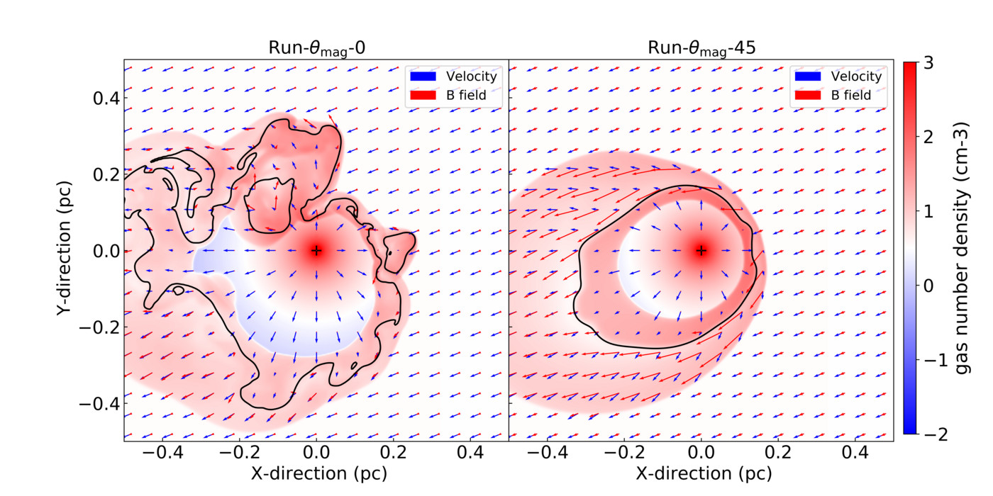
In Fig. 1 we display the number density field (in ) in the plane for models Run--0, Run--45 and Run--90, assuming different angles between the direction of motion of the star and that of the local magnetic field (a), (b) and (c), respectively. In each panel, the black contour marks the region in the astrosphere at which the mass contribution of stellar and ISM balance , respectively Meyer et al. 2017. The black cross marks the position of the star. The model Run--0 with ISM magnetic field direction parallel to that of the stellar motion recovers the hydrodynamical limit and produces an unstable bow shock exhibiting a very distorted, ragged and clumpy layer of shocked ISM material, consistent with the previous 3D hydrodynamical simulations of stellar wind bow shocks of Blondin & Koerwer 1998. The astropause, i.e. a tangential discontinuity22 2 Also called astropause, tangential discontinuity, wind-ISM interface, or pressure equilibrium surface (black line), is no more path-connected as a result of the turbulent velocity and magnetic fields in it, producing regions of ISM gas engulfed into the layer of stellar wind (Fig. 1a).
The stand-off distance of the bow shock (Baranov et al. 1971) is defined as,
| (11) |
where , standing for the gas density of the ambient medium, the ISM mean molecular weight and the proton mass. It is measured from the simulation data as (Fig. 1a-c). The stand-off distance lies on the inflow line, as Baranov et al. 1971 determined it using an incompressible irrotational fluid model, as does implicitly Wilkin 1996 who also assumes a thin-shell approach to the overall bow shock structure. The models with (Fig. 1b) and (Fig. 1c) have smoother and stable bow shock structures. Because of the extra stress and pressure provided by the ISM magnetic field, the layers of astropause and the forward shock are stabilised, see also van Marle et al. 2014, although the nebula still reveals traces of large scale eddies, repetitively advected from the apex to the tail of the bow shock (black line in Fig. 1c). The layer of shocked ISM material is enlarged and the post-shock density at the forward shock is dimmer Meyer et al. 2017.
In Fig. 2 we plot the number density field (in ) in the (left) and (right) planes in our models Run--0 (top) and Run--45 (middle) and Run--90 (bottom), assuming different angle between the direction of motion of the star and that of the local magnetic field (a,d), (b,e) and (c,f), respectively. As described above, the model with is clearly unstable and turbulent, with several knots and clumps overpassing the stand-off distance. This has been revealed in the 3D hydrodynamical simulations of the Rayleigh-Taylor and Vishiniac-unstable stellar wind bow shock modelled of Blondin & Koerwer 1998. The figures corresponding to the model with highlight that the astropause can have different stability properties can be different along distinct cross-sections such as the and planes. This induces projection effects of the nebula’s emission onto the plane of the sky, according to the viewing angle it is observed from (our Section 3.3).
Fig. 3 further illustrates the density fields in the plane of models Run--0 (left) and Run--90 (right). The overplotted vectors fields highlight the gas velocity (blue) and the magnetisation (red) of the plasma. On e sees the isotropic stellar wind flowing from the central black cross marking the position of the star, to the tangential discontinuity (thin black line). The size of the vectors scale with the magnitude of the field they represent. Hence, the Parker magnetic field in the stellar wind, several orders of magnitude smaller than that of the ambient ISM, are not visible at the naked eye in these figures. The velocity field is reduced in the post-shock region at the forward shock, as testifies the smaller blue arrows, which re-accelerate in the winged region of shocked ISM behind the apex of the astrosphere, see also our discussion on the Mach number in Section 3.2. Similarly, the ISM magnetic field is compressed in the wings of the bow shock, filled with shocked ISM material (right panels of Fig. 3).
Fig. 4 compares the analytic solution of Wilkin 1996 with the density field (in ) of the bow shock in our simulation model Run--90. The figure displays a cross-section through the plane and Wilkin’s solution is added as colored coutours representing the approximation for the morphology of an infinitely thin bow shock. It reads,
| (12) |
with is the angle between the direction of stellar motion in degrees and the stand-off distance (Eq. 11). The black contour corresponds to the stand-off distance derived from the observations of surroundings of IRC-10414 (Gvaramadze et al. 2014), while the green contour fits the astropause (marked with blue thin contour). A couple of remarks naturally arise from this comparison. First, the analytic approximation for bow shocks around red supergiant stars matches well the overall circumstellar structure. It is therefore suitable, e.g. for observers constraining the geometry of observed nebulae. However, it does not corresponds to a characteristic layer of the bow shock, such as the tangential discontinuity, for angles -. Its applicability is therefore limited to the apex of the bow shock (Blondin & Koerwer 1998; Mohamed et al. 2012).

3.2 Bow shock internal properties
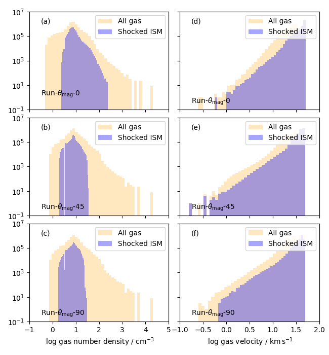
Fig. 5 shows the distribution of the gas density (right) and gas velocity (left), for both all gas in the bow shock nebulae (yellow) and for the shocked ISM gas component (blue), respectively. Figures are displayed for different angles, namely, (top), (middle) and (bottom). Gas number density (in ) and velocity (in ) are plotted in log- scale, while the distribution represents the number of grid zones which is a measure of the volume. Inspection of the left panels reveals that the inclination of the ISM magnetic field induces notable differences in the bow shock density distribution between the models, see e.g. models with (Fig. 5a) and with (Fig. 5b). Indeed, the unstable model in the hydrodynamical limit (Fig. 5a) has a density distribution which is globally larger than in the other models (Fig. 5b,c). This illustrates the well-know effect of magnetic fields in dimming the gas density in post-shock region at the forward shock (Meyer et al. 2017). Note that density distribution peaks are similar in all three models (Fig. 5a-c) as each bow shock model is driven by the same star. Not much difference is noticeable between the models with and , suggesting also that their respective maximal emissivity might not greatly differ compare to the case with (see Section 3.3).
The right panels display histogram for the gas velocity distributions in the astrospheres. The similar upper part of all distributions (Fig. 5d-f) in each panels comes from the fact that all simulations have the same central star expelling the same winds, moving at the same space velocity through the same ISM. Only mild differences are found in the low-velocity region of the two distributions, because of the changes in the velocity field in the post-shock region at the forward (bow) shock and at the reverse (termination) shock, respectively The more the flow is laminar in the shocked ISM (the less the tangential discontinuity is unstable) the lower will be the minimum gas velocity (Fig. 5e). This may have observational consequences, e.g. on atomic and molecular line emissions of the nebula, which is much beyond the scope of this study.

In Fig. 6 we further illustrate the internal structure of the stable bow shock in our model Run--. The plot is a three-dimensional rendering of the astrophere around the runaway red supergiant star IRC-10414. Transparent clipped number density surfaces render the bow shock structure and streamlines mark the magnetic field (yellow) and velocity fields (red), respectively. It shows how the stellar magnetic field, initially made of a Parker spiral transported with the stellar wind in the equatorial plane of the star, fills the entire region of freely-expanding, accelerated unshocked stellar wind. These field lines do not reconnect with the ISM magnetic field lines that penetrate the forward shock and stabilise the astropause, but rather expand as a wider spiral in the tail of the bow shock. The gas streamlines also highlight the isotropically-outflowing stellar wind from the inner stellar boundary, which enters the region of shocked wind and bends towards the tail of the astrosphere. The ISM gas enters the bow shock in its turn and flow along the wind-ISM discontinuity.
Fig. 7 displays the temperature field (top panels), sonic Mach number field (middle top panels), Alfévnic Mach number field (middle top panels) and fast magnetosonic Mach number field (middle bottom panels) in the plane of our bow shock models, displayed as a function of (left), (middle) and (right). The black contour is astropause interface of the bow shock, i.e. the location of the nebula made of equal proportion of stellar wind and ISM material (). On each panel the cross marks the position of the star. The temperature maps illustrate that the maximum temperature is at the bow shock, where it exceeds that at the termination shock (Fig. 7a-c), see also Meyer et al. 2017.
The series of panels on the Mach number,
| (13) |
shows that the gas is supersonic in the free-streaming wind and in the unshocked ISM gas, respectively. Indeed, the accelerated stellar wind is larger than the radially-decreasing temperature by adiabatic cooling , and everywhere in the unperturbed ISM. The gas is sub-sonic in the shocked regions, both located downstream the termination shock and the bow shock, as a result of the changes in both the post-shock temperature and velocity (). This permits us to clearly classify the astrosphere of IRC-10414 as a bow shock, instead of other circumstellar structures such as bow wave or dust waves which can by produced around moving stars (Pogorelov et al. 2017; Henney & Arthur 2019c). Note also that the sonic Mach number increases in the region of shocked stellar wind gas in the in wings of the bow shock (Fig. 3e,f).
The Alfénic Mach number is defined as,
| (14) |
and the fast-magnetosonic Mach number reads as,
| (15) |
with the fast-magnetosonic speed,
| (16) |
where is the angle between the gas velocity and magnetic field vector fields. Note that the sound speed is the characteristic dynamical quantity of an hydrodynamical simulation, whereas the fast-magnetosonic speed is the relevant dynamical quantity of an magneto-hydrodynamical model, respectively. Expanding stellar wind and unperturbed ISM are supersonic, super-Alfénic and super-fast magnetosonic. The values of the sonic Mach number is lower in the shocked wind region than in that of the shocked ISM gas because the post-shock gas velocity at the termination shock is smaller than at the forward shock, and because the sound speed is larger in that dense region of shocked wind (Fig. 7a-c). Similarly, the Alfénic Mach number is smaller in the shocked ISM region at the apex of the bow shock than in the layer of shocked stellar wind, because of both the changes in compressed magnetic field lines and gas number density (Fig. 7h,i). The fast-magnetosonic Mach number is below unity in all shocked regions of the stable bow shocks but larger than unity in the freely streaming stellar wind and in the ambient medium, as described in Scherer et al. 2020.
Fig. 8 shows cross-sections in the number density and Mach number fields taken through the maps displayed in Fig. 7, measured along the directions. The stellar wind density profile is clearly visible at the origin of the domain, which decreases to values that are lower in the part of the figure than in the , in the region of the bow shock opposite of the direction of stellar motion. The sonic Mach number profile reflects the decrease of the temperature in the stellar wind under the effect of adiabatic cooling while the the external photo-heating accelerates the stellar wind (Fig. 8d), see also (Meyer et al. 2014; Mackey et al. 2014), from the inner stellar wind region that is excluded from the computational domain, to the termination shock of the bow shock. As expected and above described, the fast magnetosonic Mach number number diminishes and is in the post-shock layers of materials located between the termination shock and the bow shock (Fig. 8c).


3.3 Emission maps
We produce emission maps using the radmc-3d code (Dullemond 2012), which permits calculating radiative transfer for analytic prescription of emission coefficients such as optical H optical emission. In Fig. 9, we plot H emission maps of our bow shock model Run--0. The figure displays the surface brightness (in ) of a nebula located at a distance of , corresponding to the IRC-10414 distance (Gvaramadze et al. 2014). The projected emissivity is shown under several considered rotation of the polar and azimuthal viewing angles, respectively. The white cross marks the position of the runaway star. The bow shock of the model Run--0 results turbulent. Its exhibits a diffuse nebula morphology, showing several filaments and knots dispersed around the central object. The star is much brighter than its surroundings, which raises the question of the saturation of observed fluxes and of the screening of red supergiant bow shocks.
A series of two arcs is visible ahead of the star, roughly in the direction of stellar motion (Fig. 9a). However, the star is not at the geometrical centre of the arc and some clumps are much beyond the bow shock (Fig. 9a-c). Note that this structures are very different from the circular ones obtained with 2D hydrodynamical simulations in Meyer et al. 2014. The images with are brighter than that with by a factor ?, as expected from previous 2D simulations. This behaviour is because the line-of-sight intercepts more dense material and consequently produces brighter surface brightness (Fig. 9d-f). The observed star-arc distance (called stand-off distance in the observational literature) varies significantly between models, some of them revealing distorted and clumpy arcs close to the star (Fig. 9d). The changes in the bow shock morphology are important for mild changes in the viewing angle (Fig. 9e). In these conditions, it is very difficult to distinguish a circumstellar structure, and even more uneasy to identify bow shocks, if at all, although the nebula has formed and exist (Fig. 9).
In Fig. 10, we display H emission maps of our astrosphere model Run--45. The projected emissivity morphology is very different than in the case with , as evident bow shock morphologies are visible in each panel of the figure. The maximum emission originates from the sub-sonic and super-Alfénic region of shocked stellar wind, much denser than the compressed magnetised ISM material, plus a lighter overarching arc tracing the forward shock of the bow shock. Bright clumps appear in the shocked wind close to the region of maximum emission (Fig. 10a-c). This fact reflects the instabilities at the interface between wind and ISM material visible in the plane (black line in Fig. 2b). These infrared bow shocks are not strictly symmetric with respect to the direction of motion of the star, as a consequence of the inclined magnetic field direction inducing extended wing-like regions of shocked ISM gas of different size (Fig. 2b). By projection effects, these regions can produce brighter zones wrongly suggesting, from a purely observational point of view, the presence of filaments, while it relies large-scale instabilities in the astropause interface. High-resolution simulations would result in qualitatively different patterns, and this should be explored in future works. This structure can also appear as stripes normal to the direction of motion of the runaway star (Fig. 9e,f) difficult to interpret from the observational point of view. As in Fig. 9 the surface brightness of the astrosphere is more significant with than with . Finally, note that some models are also very smooth (Fig. 9h) and fit well with the 2D predictions of Meyer et al. 2014, see Section 4.3.
In Fig. 11, we show H emission maps for our bow shock model Run--90. The situation is similar to that in our model Run--45. Several shapes arise from projection effects, with differences in the maximum emission of the circusmtellar material (Fig. 11a). Very smooth shells (Fig. 11h) or irregular (Fig. 11d,g,i) patterns of dense shocked stellar wind are mostly consequences of the unstable tangential discontinuity. Interestingly, the perpendicular orientation of the ISM magnetic field can result in series of multiple arcs normal to the direction of motion of the star (Fig. 11f) as modelled in the context of hot OB stars in Katushkina et al. 2017; Katushkina et al. 2018, see also Baalmann et al. 2021. Furthermore, the opening of the bow shock can significantly differ from a projection model to another, with rounder termination shocks (Fig. 11f) and wider arcs (Fig. 11d). Overall, our emission maps reveal the importance of projection effects in the appearance of stellar wind bow shocks from runaway red supergiant stars at H. It supports the use of astrometric measures, such as Gaia in order to determine the direction of proper motion of runaway stars instead of their circumstellar bow shocks, the latter being a source of errors resulting from the random orientation of projected astrospheres, see Peri et al. 2015.
4 Discussion
In this section, we discuss the limitations of our simulation method. As application, we reproduce the bow shocks of two runaway red supergiant stars, IRC-10414 and Betelgeuse (see below), respectively. Last, we discuss our findings in the context of nebulae around other massive stars and core-collapse supernova remnants.
4.1 Model limitation
Our 3D MHD simulations are a leap forward in studying the circumstellar medium of runaway late-type (super)giant stars, as it includes both stellar and ISM magnetic fields within a three-dimensional framework, completed with radiative transfer calculations. Therefore, the simulations are intrinsically more realistic, for example in terms of development and damping of instabilities in the bow shock structure, compare to that previously conducted in, e.g. Meyer et al. 2014. Mainly, it is possible to explore and study the effects of an ISM magnetic field that is not aligned with the direction of stellar motion, which latter configuration was imposed by the two-dimensional cylindrical coordinate system used in the other studies of that series and in van Marle et al. 2014. We study this effect by varying the angle between the direction of stellar motion and the direction of the ISM magnetic field. Our results stress the stabilising role of the ISM magnetic field already noticed in 2D precedent works with (van Marle et al. 2014; Meyer et al. 2017).
Nevertheless, within the stellar wind properties of IRC-10414, the damping of instabilities in stellar wind bow shocks is very efficient in 3D only if a few degrees, while simulations with recovers the hydrodynamical, unmagnetised limit (Fig. 13). These latter results have different stability properties than the 2D models of Meyer et al. 2014. This effect is a noteworthy difference between our 3D simulations and precedent 2D works in the context of the surroundings of IRC-10414. We interpret this difference as originating from the dissimilar coordinate systems used in these two works. The first one employs a cylindrical two-dimensional coordinate system which possesses a symmetry axis affecting the development of instabilities and leading to the complex topology of the bow shock apex (Comerón & Kaper 1998; Meyer et al. 2017). The second one considers a 3D Cartesian coordinate system, which permits circumventing that issue (Mignone 2014).
The spatial resolution of the simulations has become an essential parameter regarding the development of bow shock instabilities (van Marle et al. 2014). In that sense, future simulations should consider simulation models with even higher spatial resolution. However, one should keep in mind that fully resolving Rayleight-Taylor-based instabilities can not be achieved numerically using Eulerian codes (Blondin & Koerwer 1998; Mohamed et al. 2012), and that tending to such result would be at prohibitive numerical costs. Furthermore, our models does not include all microphysical mechanisms at work in the circumstellar medium of late-type giant stars, such non-ideal MHD processes like Ohmic diffusion and Hall effect, known to affect the density of magnetised plasmas, chemical reactions at work in the shocked enriched stellar winds or acceleration of stellar wind electrons and protons at the termination shock of bow shock nebulae (del Valle & Pohl 2018). Apart from lacking physical processes, our choices regarding boundary and initial conditions for stellar wind and the ISM will be studied in a future parameter study.
Indeed, the present study is tailored to the runaway red supergiant IRC-10414, which surface properties have been constrained by means of observations (Gvaramadze et al. 2014) completed with numerical simulations (Meyer et al. 2014). Our models, therefore, do not include stellar evolution as wind boundary conditions, e.g. time-dependently interpolating evolutionary tracks (Brott et al. 2011; Szécsi et al. 2020), which would permits to better treat the surroundings of red supergiant stars (Mackey et al. 2012; Meyer et al. 2014). On the other hand, the stellar evolution can be useful, to model core-collapse supernova remnants from - massive runaway progenitor stars (Katsuda et al. 2018). Additionally, the manner of the surrounding medium remains rather simplistic in our study as we assume a uniform, warm and ionized ISM. A natural improvement will assume a more realistic turbulent, inhomogeneous (Walch et al. 2011) and clumpy (Baalmann et al. 2021) medium. This would account for the intrinsic turbulence driven by the stellar winds of neighbouring massive stars and/or travelling shock wave from supernova remnants (Peters et al. 2017; Seifried et al. 2018).
4.2 Grid-induced effects on bow shock instability
Previous 3D Eulerian numerical works on stellar wind bow shock showed that instabilities develop along the and axis when the star moves along the axis (Blondin & Koerwer 1998). In order to avoid such an effect, our simulations impose the star a trajectory which does no coincide with a preferential direction of the 3D Cartesian coordinate system (, and ). Our direction of stellar motion makes arbitrary angles with the planes and , respectively. In Fig. 12, we plot a series of two models labelled Run-test-1 and Run-test-2 (Tab. 1), which compare the above discussed grid effects. We carry out these tests within the hydrodynamical limit (). The difference lies in the direction of the stellar motion imposed by the outer boundary conditions at the planes , and , respectively. In Run-test-1 the star moves along the axis while in Run-test-2 it moves along an arbitrary direction as described above.
The most important differences are the changes in the topology of the different discontinuities present in these cross-sections. The termination shock, astropause interface and forward shock are spherically symmetric in Run-test-1 (Fig. 12a) while absent in Run-test-2 (Fig. 12b). This fact reflects different faster-growing modes at work in the two simulation tests, it confirms the findings of Blondin & Koerwer 1998 and it illustrates the necessity to impose the star a direction of motion which does not coincide with any Cartesian axis unless grid-induced regular patterns such as the mode of Fig. 12a will develop in the shocked stellar wind. Although both are physical, Run-test-2 is closer to what would happen in nature. The isothermal stellar wind bow shock of Blondin & Koerwer 1998 concerns a slow-, dense-winded star, moving with velocity that develops a ragged, unstable, clumpy circumstellar structure. Their fig. 9 and 10 show the bow shock structure strongly influenced by the grid during many crossing-time of the ISM flow through the computational domain before becoming turbulent. Our method permits us to eliminate these grid effects without waiting for many flow times and reduce computational costs.
4.3 Comparison with observations


4.3.1 The case of IRC-10414
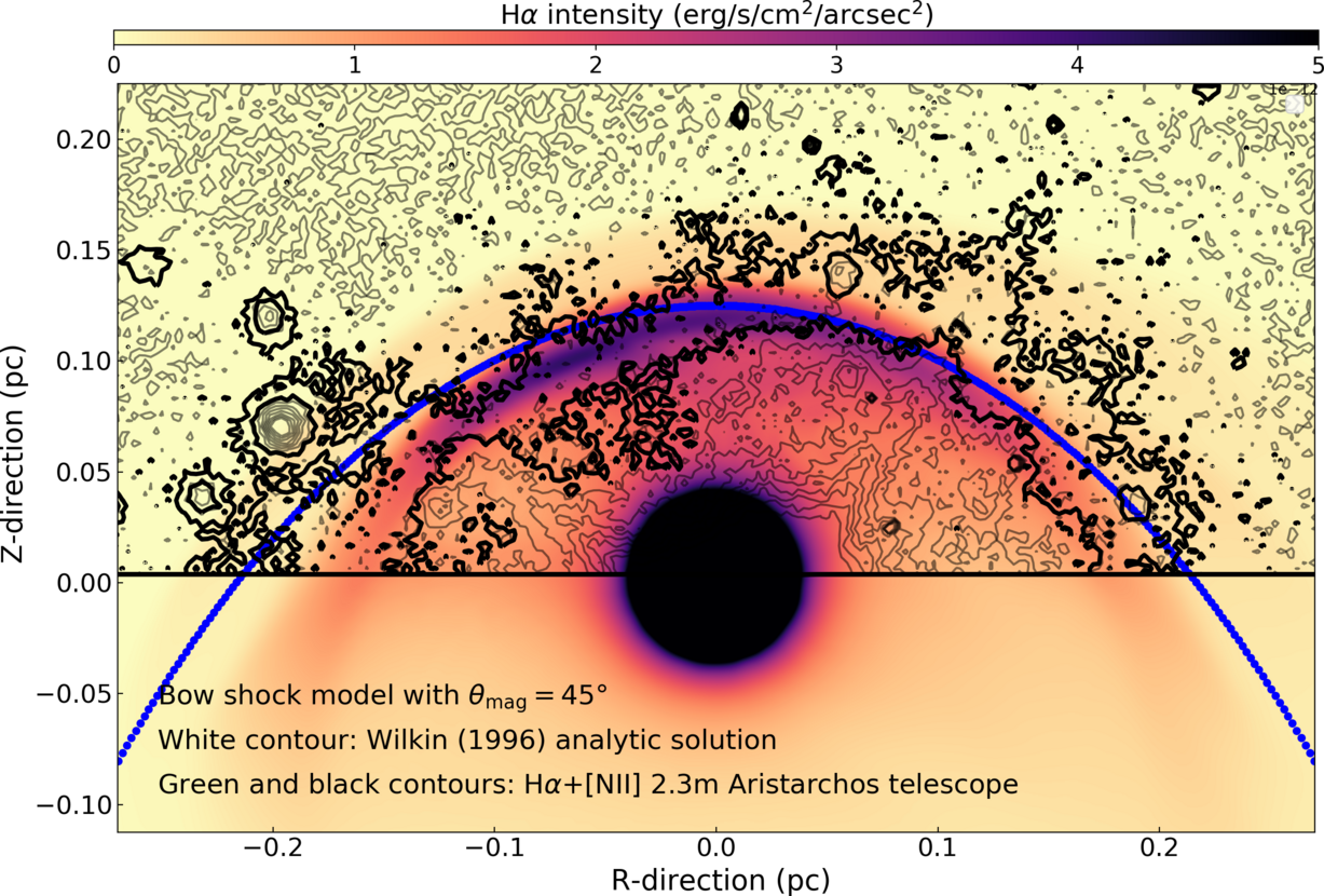
For the sake of completeness, we perform a comparison with observations between our modelled bow shock, which stellar wind properties are tailored to that of IRC-10414, and observational data of that particular circumstellar nebula. In Fig. 14, we plot a synthetic image of the simulation model Run--45 generating a stable nebula, as seen at the optical H emission line with a viewing angle characterised by and and which emission maps has been rotated so that the symmetry axis of the bow shock fits with the vertical axis of the plot. The figure additionally shows several contours from the observations taken by the Aristarchos telescope from the National Observatory of Athene (NOA) located at Mt Helmos, Greece (2326 meters above sea level). The data have been acquired via a single 30 minutes exposure, on August 9th, 2013. The thin black lines are several H+[NII] surface brightness isocontours highlighting the image background sky, and two thick black isocontours trace the arced circumstellar nebulae of IRC-10414. Last, the blue contour marks the analytic solution derived by Wilkin 1996. The data do not extend under as the telescope aperture was chosen to screen part of the star.
The observed bow shock is stable in the sense that no large-scale instabilities have developed. However, overplotted isocontours indicate that the flux is in some region of the nebula somewhat diffused. Perhaps this is caused by contamination from the starlight or background field sources, e.g. in the and part of the image. Despite of good qualitative agreements between our predictions and observations, the curvature of the bow shock is not the same in the and regions of the figure. This difference may rely on projection effects that our models do not reproduce, and better fine–tuning of our simulations would be necessary to address this question beyond the scope of our study, see Baalmann et al. 2021 for a first attempt. Therefore, even more, complex 3D MHD models are necessary to fit the data better, e.g. considering local variations in the ambient medium density and/or the turbulent character of the medium the star moves in. We chose to fit the data by matching the region at the left part ahead of the apex of the bow shock. However, we could have chosen to further rotate the nebula and fit one of our radiative transfer model with the region at the right of the apex of the bow shock, which would have engendered simulation/observations discrepancies in the left-hand part of the structure. This argument is strengthened by the blue contour representing Wilkin’s solution and consistent with only a part of the observed bow shock. Overall, our relatively good comparison with observations stresses that the bow shock of IRC-10414 is probably in a steady state. In other words, the star might have probably entered the red supergiant phase more than ago, which corresponds to the crossing-time of the simulation.
4.3.2 The case of Betelgeuse
Betelgeuse (Orionis) is the Earth-closet red supergiant star located in Orion’s neighbouring massive star-forming region. It is a runaway stellar object which displays a parsec-scale bow shock (Noriega-Crespo et al. 1997). This object is a laboratory to study the physics of cool stellar winds such as dust and test stellar pulsations models of these variable stars. Betelgeuse is the priority target of active researches on photometric variability of cool stars such as red supergiant and asymptotic giant branch stars. These works permitted the monitoring of Betelgeuse’s lightcurve and its Great optical Dimming (Dupree et al. 2020; Levesque 2021) together with measures of its magnetic field (Mathias et al. 2018; Montargès et al. 2021). Its intriguing circumstellar medium constituted of a stellar wind bow shock, an bright inner ring and a more extended, unexplained bar makes it an interesting target for hydrodynamical modelling. Previous studies on the surrounding of Betelgeuse taught us that it is a runaway star which probably experienced a blue loop. It was recently returned to the red supergiant phase (Mackey et al. 2012), leaving behind its precedent blue supergiant bow shock after briefly forming Napoleon’s hat (Wang et al. 1993). The youngness of its stellar wind bow shock is also the main conclusion of the work of Mohamed et al. 2012, presenting 3D hydrodynamical Lagrangian simulations tailored to the surroundings of Orionis. The smooth appearance of the astrosphere of Betelgeuse contradicting some simulation model ofMohamed et al. 2012. The inhibition of Rayleight-Taylor instabilities growing at the dense tangential discontinuity interface has been studied with 2.5D MHD simulations in van Marle et al. 2014, showing that the ambient magnetic field of Orion’s arm is sufficiently strong to reduce and damp the instabilities in the bow shock around Betelgeuse and modify its appearance. As for the astrosphere of IRC-10414, Betelgeuse is externally photoionised. The radiation pressure from the ionized ISM confines each of the H ii region of Betelgeuse, where the cool wind meets its hot accelerating wind within a neutral shell, is therefore located inside of the termination shock of the bow shock (Mackey et al. 2014).
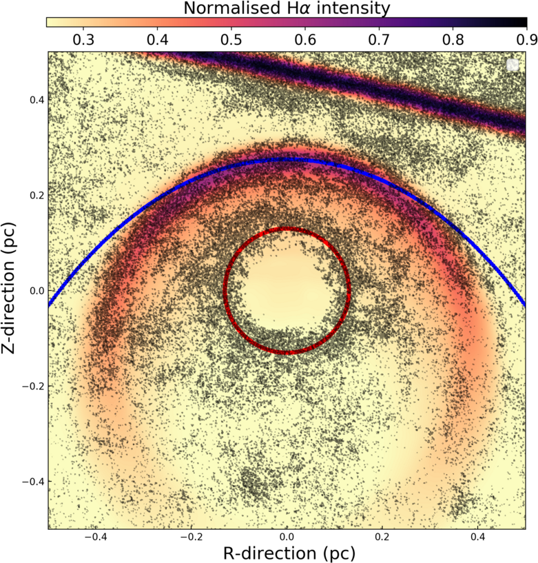
To further validate our method, we perform an additional 3D MHD simulation of Betelgeuse’s astrosphere by adopting the parameters of van Marle et al. 2014. In our simulation Run-Ori, the mass-loss rate of the star is , the stellar wind velocity is and its space velocity , respectively. The ISM ambient medium has a density , and we consider, as for IRC-10414, that its circumstellar medium is externally-ionized. Apart from the stellar wind and ISM properties, the numerical setup is the same as for IRC-10414. We adopt , i.e. we assume that the ambient medium magnetic field lines are nearly parallel to Betelgeuse’s bar. The surroundings of Betelgeuse is more complex than that of IRC-10414. Hence, we proceed differently as in Fig. 14. Betelgeuse’s bowshock is not visible in H because the star is too bright and its young nebulae too small; we mask the material that is inside of the photoionised-confined shell (also not modelled) extending up to radius . The bar is added as a denser region of Gaussian density profile peaking at and inclined with the direction of stellar motion with an angle that we adjust so that projected emission fits infrared observations. Fig. 15 compares an H emission map of the bow shock of Betelgeuse and its bar, with overlaid PACS Herschel33 3 ESA Herschel Science Archive Observation ID: 1342242656. infrared data (black contours). The blue contour is Wilkin’s solution for the bow shock morphology calculated with the observed stand-off distance of Betelgeuse’s astrosphere, whereas the red circle marks the location of the neutral shell forming at the neutral-ionized wind interface (Mackey et al. 2014). The projected bow shock structure matches well the infrared emission and we conclude that our simulation model for Betelgeuse as a old red supergiant star which astrosphere is magnetically stabilized is a probable explanation for the circumstellar medium of that star. We do not need any stellar argument to explain the bar that we treat as independent from the astropause interaction region, without any stellar evolution argument at the origin of the formation of, e.g. a double bow shock structure of Mackey et al. 2012. The concavity of the bar, slightly opposite of that of the astrosphere (Noriega-Crespo et al. 1997; van Marle et al. 2014, see), leads us to interpret the bar as of circumstellar origin, which supports the conclusions of Decin et al. 2012. The bow shock and Betelgeuse’s bar result on a serendipitous disposition and projection effects from both components.
Last, this radiative transfer modelling for the surroundings of Betelgeuse calls a few comments. First, concerning the selected simulated snapshot that we decided to produce Fig. 15. We took the youngest bow shock which aspect ratio is consistent with Betelgeuse’s observed one, measured to and (Mohamed et al. 2012; van Marle et al. 2014). It consists to the time instance after the onset of Run-Ori, when the physical size of the astropshere corresponds to that derived in Noriega-Crespo et al. 1997. The aspect ratio persists up to . At the same time, the nebula grows, i.e. bow shocks at a later time will still reasonably match the Herschel observations, however, at the cost of reevaluating the distance to the star. Secondly, the adopted inclination angle of the Betelgeuse bow shock with respect to the plane of the sky. For the sake of simplicity, when generating the initial conditions for the radiative transfer calculation, we have assumed an inclination angle of . Further modelling with the radmc-3d code indicates that no noticeable differences appear for inclination angles . However, for angles the H bow shock experiences significant projection effects, as already noted using column densities by Mohamed et al. 2012, see also our Fig. 16.

4.4 Implication for other astrophysical objects
4.4.1 Implication for bow shocks around OB stars
The many projection effects at work in our optical H emission maps of bow shocks around runaway red supergiant stars (Figs. 9-11) can be discussed in the context of earlier-type massive stars. Various catalogues of arc-like nebulae have been established, principally in the infrared waveband of the electromagnetic spectrum (van Buren & McCray 1988; van Buren et al. 1995; Noriega-Crespo et al. 1997; Peri et al. 2012; Peri et al. 2015; Kobulnicky et al. 2010; Kobulnicky et al. 2016; Kobulnicky et al. 2017). Many astrospheres around those main-sequence massive OB stars display partly irregular shapes, making their detailed classification difficult, redundant and uneasy. At the light of the emission maps of our 3D MHD simulations, we propose that other bow shocks are affected by similar projection effects, and that the peculiar morphology of some bow shocks around earlier-type massive stars are hence produced. This would greatly reduce the taxonomy of different physical morphologies of astrospheres.
4.4.2 Implication for core-collapse supernova remnants
Besides constraining stellar evolutionary parameters, the prime importance for the study of the surroundings of evolved massive stars is their role as the pre-supernova circumstellar medium of core-collapse supernova progenitors (Borkowski et al. 1992; Velázquez et al. 2006; Toledo-Roy et al. 2014; Broersen et al. 2014; Chiotellis et al. 2019; Chiotellis et al. 2021). After the explosive death of a massive star, the supernova shock wave will inevitably interact with its pre-shaped surroundings, which, according to the mass that is trapped into it (Meyer et al. 2015), first potentially feel its presence from the dynamical point of view, generate an asymmetric supernova remnant and eventually further expand into the ambient medium (Meyer et al. 2020). Inversely, the morphology of core-collapse supernovae remnants permit to constrain the properties of its circumstellar medium, itself function of the past evolution of the progenitor star. A significant fraction of massive stars being runaway stellar objects, a similar fraction of core-collapse supernova remnants must have been shaped, or at least must have at some time beard imprints of their progenitor’s bow shock, driven either by a red supergiant or a Wolf-Rayet star (Katsuda et al. 2018). Therefore, the expanding supernova shock wave properties will be completely different once it has passed through its circumstellar medium, and this will affect, e.g. particle acceleration mechanisms therein. Carefully understanding cosmic-ray acceleration in core-collapse supernovae requires an accurate treatment of its ambient medium prior to the explosion, and our work shows that this should be performed by means of 3D MHD simulations.
5 Conclusion
In this study, we explore the morphology and emission properties of the astrosphere generated around a runaway evolved, cool massive star. We present the first 3D MHD simulations of bow shocks forming in the vicinity of a runaway supergiant star, tailoring our simulations devoted to the surroundings of the M-type star IRC-10414 (Gvaramadze et al. 2014; Meyer et al. 2014). Our numerical simulations are 3D Cartesian models performed with the pluto code (Mignone et al. 2007; Mignone et al. 2012; Vaidya et al. 2018), a well-tested tool for modelling astropause interactions (Meyer et al. 2017). Constant adopted stellar wind properties are that of IRC-10414, constrained in Gvaramadze et al. 2014 and Meyer et al. 2014, and we assume that the ISM in which the star moves is supported by a typical magnetic field of strength . Our free parameter is the orientation of the ISM magnetic field with respect to the direction of stellar motion. We run a simulation for , which corresponds to a few dynamical crossing-time of the gas throughout the computational domain. For the sake of completeness, stellar rotation and magnetic field are included into the numerical setup as a Parker spiral. This 3D MHD study, therefore, permits exploring the effects of a non-aligned magnetic field on the structure and emission properties of the resulting stellar wind bow shock.
Magnetic fields stabilise astrospheres (van Marle et al. 2014; Meyer et al. 2017; Scherer et al. 2020). Mainly, when the local ISM magnetic field is aligned with less than a few degrees with that of the stellar motion, the bow shock is ragged, clumpy and strongly unstable, while previous 2D simulations produced stable structures (Meyer et al. 2014). Axisymmetric patterns are broken, principally because of large scale 3D eddies developing at the astropause interface and affecting the overall morphology of the bow shock wings. Grid-induced effects are at work when the star moves along a characteristic axis of the 3D Cartesian coordinate system, while they vanish when the stellar motion is directed along an arbitrary direction. Such results stress the need for 3D MHD simulations in further tackling the problem of the circumstellar medium of massive stars (van Marle et al. 2015b). We find that the stellar magnetic field is dynamically unimportant in shaping the astrosphere of evolved, red supergiant, massive stars, which is consistent with other studies devoted to, e.g., the heliosphere (Pogorelov et al. 2017) and the study on Cephei of Scherer et al. 2020.
Synthetic optical H emission maps of 3D MHD astrospheres around cool stars show that projection effects are important in the observed shape of the nebulae, and we speculate that this must also affect the astrospheres of earlier-type massive stars. This study shows that the problem of the smooth appearance of red supergiant bow shock can be solved with a simple, mild magnetisation of its ambient medium, and that the previously proposed external ionisation and/or youth of the structure might not be enough to explain the unique appearance of both IRC-10414 and Betelgeuse, although it participates to it (van Marle et al. 2014). We conclude that IRC-10414 is a star in a steady state and that Betelgeuse’s bar is of interstellar origin. Our work is therefore in accordance with the bow shock models for Betelgeuse of Mohamed et al. 2012 and van Marle et al. 2014, but it is in clear disfavour regarding to that proposed in Mackey et al. 2012. Our results will serve for future modelling of the circumstellar medium of runaway red supergiant stars and to realistically simulate the early supernova-blastwave interaction happening in core-collapse supernova remnants.
Acknowledgements
D. M.-A. Meyer thanks L. Decin and A.-J. van Marle for advice on observational data. The authors acknowledge the North-German Supercomputing Alliance (HLRN) for providing HPC resources that have contributed to the research results reported in this paper. M. Petrov acknowledges the Max Planck Computing and Data Facility (MPCDF) for providing data storage resources and HPC resources which contributed to test and optimise the pluto code. PFV acknowledges the financial support for PAPIIT-UNAM grant IA103121. This work is based on observations made with the “Aristarchos” telescope operated on the Helmos Observatory by the Institute of Astronomy, Astrophysics, Space Applications and Remote Sensing of the National Observatory of Athens.
Data availability
This research made use of the pluto code developed at the University of Torino by A. Mignone and collaborators (http://plutocode.ph.unito.it/) and of the radmc-3d code developed by C. Dullemond and collaborators at the University of Heidelberg (https://www.ita.uni-heidelberg.de/~dullemond/software/radmc-3d/), respectively. The figures have been produced using the Matplotlib plotting library for the Python programming language (https://matplotlib.org/). The 3D renderings have been generated using the Visit software https://visit-dav.github.io/visit-website/. Observational data of the circumstellar medium of Betelgeuse have been obtained via the Herschel data Schearch of the NASA/IPAC Infrared Science Archive (https://irsa.ipac.caltech.edu/applications/Herschel/). The data underlying this article will be shared on reasonable request to the corresponding author.
References
- Acreman et al. (2016) Acreman D. M., Stevens I. R., Harries T. J., 2016, MNRAS, 456, 136
- Baalmann et al. (2021) Baalmann L. R., Scherer K., Kleimann J., Fichtner H., Bomans D. J., Weis K., 2021, A&A, 650, A36
- Baranov et al. (1971) Baranov V. B., Krasnobaev K. V., Kulikovskii A. G., 1971, Soviet Physics Doklady, 15, 791
- Benaglia et al. (2021) Benaglia P., del Palacio S., Hales C., Colazo M. E., 2021, MNRAS, 503, 2514
- Blaauw (1961) Blaauw A., 1961, Bull. Astron. Inst. Netherlands, 15, 265
- Blondin & Koerwer (1998) Blondin J. M., Koerwer J. F., 1998, New Ast., 3, 571
- Borkowski et al. (1992) Borkowski K. J., Blondin J. M., Sarazin C. L., 1992, ApJ, 400, 222
- Brighenti & D’Ercole (1995) Brighenti F., D’Ercole A., 1995, MNRAS, 277, 53
- Broersen et al. (2014) Broersen S., Chiotellis A., Vink J., Bamba A., 2014, MNRAS, 441, 3040
- Brott et al. (2011) Brott I., de Mink S. E., Cantiello M., Langer N., de Koter A., Evans C. J., Hunter I., Trundle C., Vink J. S., 2011, A&A, 530, A115
- Brown & Bomans (2005) Brown D., Bomans D. J., 2005, A&A, 439, 183
- Cannon et al. (2021) Cannon E., Montargès M., de Koter A., Decin L., Min M., Lagadec E., Kervella P., Sundqvist J. O., Sana H., 2021, MNRAS, 502, 369
- Chevalier (1977) Chevalier R. A., 1977, ARA&A, 15, 175
- Chevalier & Luo (1994) Chevalier R. A., Luo D., 1994, ApJ, 421, 225
- Chiotellis et al. (2019) Chiotellis A., Boumis P., Derlopa S., Steffen W., 2019, arXiv e-prints, p. arXiv:1909.08947
- Chiotellis et al. (2021) Chiotellis A., Boumis P., Spetsieri Z. T., 2021, MNRAS, 502, 176
- Chiotellis et al. (2012) Chiotellis A., Schure K. M., Vink J., 2012, A&A, 537, A139
- Comerón & Kaper (1998) Comerón F., Kaper L., 1998, A&A, 338, 273
- Cox et al. (2012a) Cox N. L. J., Kerschbaum F., van Marle A.-J., Decin L., Ladjal D., Mayer A., 2012a, A&A, 537, A35
- Cox et al. (2012b) Cox N. L. J., Kerschbaum F., van Marle A. J., Decin L., Ladjal D., Mayer A., 2012b, A&A, 543, C1
- Cox et al. (2012) Cox N. L. J., Kerschbaum F., van Marle A.-J., Decin L., Ladjal D., Mayer A., Groenewegen M. A. T., van Eck S., Royer P., Ottensamer R., Ueta T., Jorissen A., Mecina M., Meliani Z., Luntzer A., Blommaert J. A. D. L., Posch T., Vandenbussche B., Waelkens C., 2012, A&A, 537, A35
- De Becker et al. (2017) De Becker M., del Valle M. V., Romero G. E., Peri C. S., Benaglia P., 2017, MNRAS, 471, 4452
- Decin et al. (2012) Decin L., N. L. J., Royer P., Van Marle A. J., Vandenbussche B., Ladjal D., Kerschbaum F., Ottensamer R., Barlow M. J., Blommaert J. A. D. L., Gomez H. L., Groenewegen M. A. T., Lim T., Swinyard B. M., Waelkens C., Tielens A. G. G. M., 2012, A&A, 548, A113
- del Valle & Pohl (2018) del Valle M. V., Pohl M., 2018, ApJ, 864, 19
- Dgani et al. (1996a) Dgani R., van Buren D., Noriega-Crespo A., 1996a, ApJ, 461, 927
- Dgani et al. (1996b) Dgani R., van Buren D., Noriega-Crespo A., 1996b, ApJ, 461, 372
- Dinçel et al. (2015) Dinçel B., Neuhäuser R., Yerli S. K., Ankay A., Tetzlaff N., Torres G., Mugrauer M., 2015, MNRAS, 448, 3196
- Dolan et al. (2016) Dolan M. M., Mathews G. J., Lam D. D., Quynh Lan N., Herczeg G. J., Dearborn D. S. P., 2016, ApJ, 819, 7
- Dullemond (2012) Dullemond C. P., , 2012, RADMC-3D: A multi-purpose radiative transfer tool, Astrophysics Source Code Library
- Dupree et al. (2020) Dupree A. K., Strassmeier K. G., Matthews L. D., Uitenbroek H., Calderwood T., Granzer T., Guinan E. F., Leike R., Montargès M., Richards A. M. S., Wasatonic R., Weber M., 2020, ApJ, 899, 68
- Dwarkadas (2007) Dwarkadas V. V., 2007, ApJ, 667, 226
- Ekström et al. (2012) Ekström S., Georgy C., Eggenberger P., Meynet G., Mowlavi N., Wyttenbach A., Granada A., Decressin T., Hirschi R., Frischknecht U., Charbonnel C., Maeder A., 2012, A&A, 537, A146
- Eldridge et al. (2011) Eldridge J. J., Langer N., Tout C. A., 2011, MNRAS, 414, 3501
- Farrell et al. (2020) Farrell E. J., Groh J. H., Meynet G., Eldridge J. J., 2020, MNRAS, 494, L53
- Freyer et al. (2003) Freyer T., Hensler G., Yorke H. W., 2003, ApJ, 594, 888
- Freyer et al. (2006) Freyer T., Hensler G., Yorke H. W., 2006, ApJ, 638, 262
- Garcia-Segura et al. (1996) Garcia-Segura G., Langer N., Mac Low M.-M., 1996, A&A, 316, 133
- García-Segura et al. (2018) García-Segura G., Ricker P. M., Taam R. E., 2018, ApJ, 860, 19
- García-Segura et al. (2020) García-Segura G., Taam R. E., Ricker P. M., 2020, ApJ, 893, 150
- Gies (1987) Gies D. R., 1987, ApJS, 64, 545
- Green et al. (2019) Green S., Mackey J., Haworth T. J., Gvaramadze V. V., Duffy P., 2019, A&A, 625, A4
- Gull & Sofia (1979) Gull T. R., Sofia S., 1979, ApJ, 230, 782
- Gvaramadze (2006) Gvaramadze V. V., 2006, A&A, 454, 239
- Gvaramadze et al. (2018) Gvaramadze V. V., Alexashov D. B., Katushkina O. A., Kniazev A. Y., 2018, MNRAS, 474, 4421
- Gvaramadze & Gualandris (2011) Gvaramadze V. V., Gualandris A., 2011, MNRAS, 410, 304
- Gvaramadze et al. (2010) Gvaramadze V. V., Kniazev A. Y., Fabrika S., 2010, MNRAS, 405, 1047
- Gvaramadze et al. (2014) Gvaramadze V. V., Menten K. M., Kniazev A. Y., Langer N., Mackey J., Kraus A., Meyer D. M.-A., Kamiński T., 2014, MNRAS, 437, 843
- Harten et al. (1983) Harten A., Lax P. D., van Leer B., 1983, SIAM Review, 25, 35
- Henney & Arthur (2019a) Henney W. J., Arthur S. J., 2019a, MNRAS, 486, 3423
- Henney & Arthur (2019b) Henney W. J., Arthur S. J., 2019b, MNRAS, 486, 4423
- Henney & Arthur (2019c) Henney W. J., Arthur S. J., 2019c, arXiv e-prints, p. arXiv:1904.00343
- Henney et al. (2019) Henney W. J., Tarango-Yong J. A., Ángel Gutiérrez-Soto L., Arthur S. J., 2019, arXiv e-prints, p. arXiv:1907.00122
- Herbst et al. (2020) Herbst K., Scherer K., Ferreira S. E. S., Baalmann L. R., Engelbrecht N. E., Fichtner H., Kleimann J., Strauss R. D. T., Moeketsi D. M., Mohamed S., 2020, ApJ, 897, L27
- Hoogerwerf et al. (2001) Hoogerwerf R., de Bruijne J. H. J., de Zeeuw P. T., 2001, A&A, 365, 49
- Izmodenov et al. (2003) Izmodenov V., Malama Y. G., Gloeckler G., Geiss J., 2003, ApJ, 594, L59
- Kaper et al. (1997) Kaper L., van Loon J. T., Augusteijn T., Goudfrooij P., Patat F., Waters L. B. F. M., Zijlstra A. A., 1997, ApJ, 475, L37
- Katsuda et al. (2018) Katsuda S., Takiwaki T., Tominaga N., Moriya T. J., Nakamura K., 2018, ApJ, 863, 127
- Katushkina et al. (2018) Katushkina O. A., Alexashov D. B., Gvaramadze V. V., Izmodenov V. V., 2018, MNRAS, 473, 1576
- Katushkina et al. (2017) Katushkina O. A., Alexashov D. B., Izmodenov V. V., Gvaramadze V. V., 2017, MNRAS, 465, 1573
- Kervella et al. (2018) Kervella P., Decin L., Richards A. M. S., Harper G. M., McDonald I., O’Gorman E., Montargès M., Homan W., Ohnaka K., 2018, A&A, 609, A67
- Kobulnicky et al. (2016) Kobulnicky H. A., Chick W. T., Schurhammer D. P., Andrews J. E., Povich M. S., Munari S. A., Olivier G. M., Sorber R. L., Wernke H. N., Dale D. A., 2016, ApJS, 227, 18
- Kobulnicky et al. (2010) Kobulnicky H. A., Gilbert I. J., Kiminki D. C., 2010, ApJ, 710, 549
- Kobulnicky et al. (2017) Kobulnicky H. A., Schurhammer D. P., Baldwin D. J., Chick W. T., Dixon D. M., Lee D., Povich M. S., 2017, AJ, 154, 201
- Lada & Lada (2003) Lada C. J., Lada E. A., 2003, ARA&A, 41, 57
- Langer (2012) Langer N., 2012, ARA&A, 50, 107
- Levesque (2021) Levesque E. M., 2021, Nature, 594, 343
- Mackey et al. (2016) Mackey J., Haworth T. J., Gvaramadze V. V., Mohamed S., Langer N., Harries T. J., 2016, A&A, 586, A114
- Mackey et al. (2014) Mackey J., Mohamed S., Gvaramadze V. V., Kotak R., Langer N., Meyer D. M.-A., Moriya T. J., Neilson H. R., 2014, Nature, 512, 282
- Mackey et al. (2012) Mackey J., Mohamed S., Neilson H. R., Langer N., Meyer D. M.-A., 2012, ApJ, 751, L10
- Maeder (2009) Maeder A., 2009, Physics, Formation and Evolution of Rotating Stars, springer-verlag edn. Astronomy and Astrophysics Library
- Mathias et al. (2018) Mathias P., Aurière M., López Ariste A., Petit P., Tessore B., Josselin E. e. a., 2018, A&A, 615, A116
- Matsuura et al. (2014) Matsuura M., Yates J. A., Barlow M. J., Swinyard B. M., Royer P., Cernicharo J., Decin L., Wesson R., Polehampton E. T., Blommaert J. A. D. L., Groenewegen M. A. T., Van de Steene G. C., van Hoof P. A. M., 2014, MNRAS, 437, 532
- Meyer et al. (2014) Meyer D. M.-A., Gvaramadze V. V., Langer N., Mackey J., Boumis P., Mohamed S., 2014, MNRAS, 439, L41
- Meyer et al. (2015) Meyer D. M.-A., Langer N., Mackey J., Velázquez P. F., Gusdorf A., 2015, MNRAS, 450, 3080
- Meyer et al. (2014) Meyer D. M.-A., Mackey J., Langer N., Gvaramadze V. V., Mignone A., Izzard R. G., Kaper L., 2014, MNRAS, 444, 2754
- Meyer et al. (2017) Meyer D. M. A., Mignone A., Kuiper R., Raga A. C., Kley W., 2017, MNRAS, 464, 3229
- Meyer et al. (2020) Meyer D. M. A., Oskinova L. M., Pohl M., Petrov M., 2020, MNRAS, 496, 3906
- Meyer et al. (2020) Meyer D. M. A., Petrov M., Pohl M., 2020, MNRAS, 493, 3548
- Meyer et al. (2021) Meyer D. M. A., Pohl M., Petrov M., Oskinova L., 2021, MNRAS, 502, 5340
- Meyer et al. (2016) Meyer D. M.-A., van Marle A.-J., Kuiper R., Kley W., 2016, MNRAS, 459, 1146
- Mignone (2014) Mignone A., 2014, Journal of Computational Physics, 270, 784
- Mignone et al. (2007) Mignone A., Bodo G., Massaglia S., Matsakos T., Tesileanu O., Zanni C., Ferrari A., 2007, ApJS, 170, 228
- Mignone et al. (2012) Mignone A., Zanni C., Tzeferacos P., van Straalen B., Colella P., Bodo G., 2012, ApJS, 198, 7
- Mohamed et al. (2012) Mohamed S., Mackey J., Langer N., 2012, A&A, 541, A1
- Montargès et al. (2021) Montargès M., Cannon E., Lagadec E., de Koter A., Kervella P., Sanchez-Bermudez J. e. a., 2021, Nature, 594, 365
- Montargès et al. (2019) Montargès M., Homan W., Keller D., Clementel N., Shetye S., Decin L., Harper G. M., Royer P., Winters J. M., Le Bertre T., Richards A. M. S., 2019, MNRAS, 485, 2417
- Noriega-Crespo et al. (1997) Noriega-Crespo A., van Buren D., Cao Y., Dgani R., 1997, AJ, 114, 837
- Noriega-Crespo et al. (1997) Noriega-Crespo A., van Buren D., Dgani R., 1997, AJ, 113, 780
- O’Gorman et al. (2015) O’Gorman E., Vlemmings W., Richards A. M. S., Baudry A., De Beck E., Decin L., Harper G. M., Humphreys E. M., Kervella P., Khouri T., Muller S., 2015, A&A, 573, L1
- Parker (1958) Parker E. N., 1958, ApJ, 128, 664
- Peri et al. (2012) Peri C. S., Benaglia P., Brookes D. P., Stevens I. R., Isequilla N. L., 2012, A&A, 538, A108
- Peri et al. (2015) Peri C. S., Benaglia P., Isequilla N. L., 2015, A&A, 578, A45
- Peters et al. (2017) Peters T., Zhukovska S., Naab T., Girichidis P., Walch S., Glover S. C. O., Klessen R. S., Clark P. C., Seifried D., 2017, MNRAS, 467, 4322
- Pogorelov et al. (2017) Pogorelov N. V., Heerikhuisen J., Roytershteyn V., Burlaga L. F., Gurnett D. A., Kurth W. S., 2017, ApJ, 845, 9
- Povich et al. (2008) Povich M. S., Benjamin R. A., Whitney B. A., Babler B. L., Indebetouw R., Meade M. R., Churchwell E., 2008, ApJ, 689, 242
- Powell (1997) Powell K. G., 1997, An Approximate Riemann Solver for Magnetohydrodynamics. Springer Berlin Heidelberg, Berlin, Heidelberg, pp 570–583
- Renzo et al. (2019) Renzo M., Zapartas E., de Mink S. E., Götberg Y., Justham S., Farmer R. J., Izzard R. G., Toonen S., Sana H., 2019, A&A, 624, A66
- Rozyczka & Franco (1996) Rozyczka M., Franco J., 1996, ApJ, 469, L127
- Sander et al. (2020) Sander A. A. C., Vink J. S., Hamann W. R., 2020, MNRAS, 491, 4406
- Scherer et al. (2020) Scherer K., Baalmann L. R., Fichtner H., Kleimann J., Bomans D. J., Weis K., Ferreira S. E. S., Herbst K., 2020, MNRAS, 493, 4172
- Scherer et al. (2014) Scherer K., Fichtner H., Fahr H. J., Bzowski M., Ferreira S. E. S., 2014, A&A, 563, A69
- Seifried et al. (2018) Seifried D., Walch S., Haid S., Girichidis P., Naab T., 2018, ApJ, 855, 81
- Shrestha et al. (2018) Shrestha M., Neilson H. R., Hoffman J. L., Ignace R., 2018, MNRAS, 477, 1365
- Shrestha et al. (2021) Shrestha M., Neilson H. R., Hoffman J. L., Ignace R., Fullard A. G., 2021, MNRAS, 500, 4319
- Smartt (2009) Smartt S. J., 2009, ARA&A, 47, 63
- Szécsi et al. (2020) Szécsi D., Wünsch R., Agrawal P., Langer N., 2020, arXiv e-prints, p. arXiv:2004.08203
- Teyssier et al. (2012) Teyssier D., Quintana-Lacaci G., Marston A. P., Bujarrabal V., Alcolea J., Cernicharo J., Decin L., Dominik C., Justtanont K., de Koter A., Melnick G., Menten K. M., Neufeld D. A., Olofsson H., Planesas P., Schmidt M., Soria-Ruiz R., Schöier F. L., Szczerba R., Waters L. B. F. M., 2012, A&A, 545, A99
- Toledo-Roy et al. (2014) Toledo-Roy J. C., Esquivel A., Velázquez P. F., Reynoso E. M., 2014, MNRAS, 442, 229
- Vaidya et al. (2018) Vaidya B., Mignone A., Bodo G., Rossi P., Massaglia S., 2018, ApJ, 865, 144
- van Buren & McCray (1988) van Buren D., McCray R., 1988, ApJ, 329, L93
- van Buren et al. (1995) van Buren D., Noriega-Crespo A., Dgani R., 1995, AJ, 110, 2914
- van Marle et al. (2014) van Marle A. J., Decin L., Meliani Z., 2014, A&A, 561, A152
- van Marle et al. (2005) van Marle A. J., Langer N., García-Segura G., 2005, A&A, 444, 837
- van Marle et al. (2008) van Marle A. J., Langer N., Yoon S.-C., García-Segura G., 2008, A&A, 478, 769
- van Marle et al. (2011a) van Marle A. J., Meliani Z., Keppens R., Decin L., 2011a, ApJ, 734, L26
- van Marle et al. (2011b) van Marle A. J., Meliani Z., Keppens R., Decin L., 2011b, ApJ, 734, L26
- van Marle et al. (2012) van Marle A. J., Meliani Z., Marcowith A., 2012, A&A, 541, L8
- van Marle et al. (2015a) van Marle A. J., Meliani Z., Marcowith A., 2015a, A&A, 584, A49
- van Marle et al. (2015b) van Marle A. J., Meliani Z., Marcowith A., 2015b, A&A, 584, A49
- Velázquez et al. (2006) Velázquez P. F., Vigh C. D., Reynoso E. M., Gómez D. O., Schneiter E. M., 2006, ApJ, 649, 779
- Villaver et al. (2012) Villaver E., Manchado A., García-Segura G., 2012, ApJ, 748, 94
- Vink (2006) Vink J. S., 2006, in Lamers H. J. G. L. M., Langer N., Nugis T., Annuk K., eds, Stellar Evolution at Low Metallicity: Mass Loss, Explosions, Cosmology Vol. 353 of Astronomical Society of the Pacific Conference Series, Massive star feedback – from the first stars to the present. p. 113
- Vlemmings et al. (2002) Vlemmings W. H. T., Diamond P. J., van Langevelde H. J., 2002, A&A, 394, 589
- Vlemmings et al. (2005) Vlemmings W. H. T., van Langevelde H. J., Diamond P. J., 2005, A&A, 434, 1029
- Walch et al. (2011) Walch S., Wünsch R., Burkert A., Glover S., Whitworth A., 2011, ApJ, 733, 47
- Wang et al. (1993) Wang L., Dyson J. E., Kahn F. D., 1993, MNRAS, 261, 391
- Wareing et al. (2007a) Wareing C. J., Zijlstra A. A., O’Brien T. J., 2007a, MNRAS, 382, 1233
- Wareing et al. (2007b) Wareing C. J., Zijlstra A. A., O’Brien T. J., 2007b, ApJ, 660, L129
- Weaver et al. (1977) Weaver R., McCray R., Castor J., Shapiro P., Moore R., 1977, ApJ, 218, 377
- Weber & Davis (1967) Weber E. J., Davis Leverett J., 1967, ApJ, 148, 217
- Weiler & Sramek (1988) Weiler K. W., Sramek R. A., 1988, ARA&A, 26, 295
- Wilkin (1996) Wilkin F. P., 1996, ApJ, 459, L31
- Woosley & Bloom (2006) Woosley S. E., Bloom J. S., 2006, ARA&A, 44, 507
- Woosley et al. (2002) Woosley S. E., Heger A., Weaver T. A., 2002, Reviews of Modern Physics, 74, 1015