Randomized Benchmarking for Non-Markovian Noise
Abstract
Estimating the features of noise is the first step in a chain of protocols that will someday lead to fault-tolerant quantum computers. The randomized benchmarking (RB) protocol is designed with this exact mindset, estimating the average strength of noise in a quantum processor with relative ease in practice. However, RB, along with most other benchmarking and characterization methods, is limited in scope because it assumes that the noise is temporally uncorrelated (Markovian), which is increasingly evident not to be the case. Here, we combine the RB protocol with a recent framework describing non-Markovian quantum phenomena to derive a general analytical expression of the average sequence fidelity (ASF) for non-Markovian RB with the Clifford group. We show that one can identify non-Markovian features of the noise directly from the ASF through its deviations from the Markovian case, proposing a set of methods to collectively estimate these deviations, non-Markovian memory time scales, and diagnose (in)coherence of non-Markovian noise in an RB experiment. Finally, we demonstrate the efficacy of our proposal by means of several proof-of-principle examples. Our methods are directly implementable and pave the way for a better understanding of correlated noise in quantum processors.
I Introduction
The biggest challenge faced in any quantum computation can almost unequivocally be said to be the presence of errors. Among these, noise arising from interactions with the surroundings of a system represent an important class that is still far from being well understood. Given the current widespread interest in designing complex fault-tolerant quantum systems, together with the fundamental restriction that no system can ever be fully isolated from its surroundings, the need to advance our understanding of this type of noise cannot be understated.
Over the last decade, the approach known as randomized benchmarking (RB) Emerson et al. 2005; Lévi et al. 2007; Knill et al. 2008; Magesan et al. 2011; Magesan et al. 2012a has become the gold standard to certify the performance of gate sets and characterize the noise in computations involving these sets. RB generally refers to an experimental protocol allowing estimation of error rates of a gate set by quantifying their control fidelity as a function of the number of gates Helsen et al. 2020. Moreover, it does so in an efficient way that is robust to state preparation and measurement (SPAM) errors, as opposed to approaches such as quantum process tomography (QPT) Chuang and Nielsen 1997. It is important to point out, however, that the two approaches are rather complementary Roth et al. 2018, as RB extracts less information about the noise, namely average error rates of average gates, but requires little resources for high confidence Wallman and Flammia 2014, while QPT allows to fully reconstruct noise but with a higher resource cost Mohseni et al. 2008. Aside from QPT and RB, there is a plethora of other methods lying in between, such as gate set tomography Nielsen et al. 2020, compressed sensing Gross et al. 2010; Flammia et al. 2012 or direct fidelity estimation Flammia and Liu 2011; da Silva et al. 2011; Moussa et al. 2012, to name a few, to characterize quantum devices. The main reason why RB has become an essential tool for quantum technologies is thus its practicality and applicability to realistic experimental settings.
The most common versions of RB protocols are executed for sequences of Clifford gates Knill et al. 2008, and consider noise that is both time and gate independent, in particular Markovian and context independent. In this case, it is observed that the so-called average sequence fidelity (ASF), i.e. a figure of merit relating to the gate fidelity of the noise11 1 In Ref. Proctor et al. 2017, it was pointed out that this relation between the ASF and the gate fidelity of the noise is not unique due to gauge invariance. An in-depth discussion can be seen in Ref. Wallman 2018; Merkel et al. 2018 with an overview and generalisation in Helsen et al. 2020., behaves as a decaying exponential in the number of gates applied in the sequence. Nevertheless, progress for time-dependent Wallman and Flammia 2014 and gate-dependent noise Proctor et al. 2017; Wallman 2018; Helsen et al. 2019, as well as different gate sets Carignan-Dugas et al. 2015; Hashagen et al. 2018; Helsen et al. 2019 or other figures of merit has also been made Magesan et al. 2012b; Wallman et al. 2015. Despite this, RB has generally remained elusive to a characterization in the presence of temporally-correlated, so-called non-Markovian noise, and has rather been identified when the ASF does not behave as a decaying exponential in numerical and experimental studies Ryan et al. 2009; Park et al. 2016; Epstein et al. 2014; Fogarty et al. 2015; Mavadia et al. 2018. Hence it is not an overstatement that overcoming the Markovianity assumption in RB remains one of the most important hurdles to clear towards fault tolerance in quantum computers.
Correlated noise has been thoroughly examined in particular scenarios, such as that of dephasing noise. For classical correlations, e.g. in Ref. Ball et al. 2016; Mavadia et al. 2018 (and similarly in Ref. Fong and Merkel 2017), the noise is modeled as rotations of a qubit around the -axis as determined by a classical random variable, and deviations from the uncorrelated case are found. For the quantum counterpart, in Ref. Qi and Ng 2021 this is generalized to correlations being mediated by a bath, modeled as a multi-mode bosonic field interacting with the qubit. Similarly, correlations arising as interaction between neighboring qubits, so-called crosstalk Gambetta et al. 2012 have been addressed in multi-qubit RB protocols, generally noticing that averaging over a single qubit generally leads to a non-exponential decay of the ASF.
The study of temporal correlations in quantum systems necessarily require in its foundations a theory of quantum stochastic processes. The development of such a theory has much older origins than RB but has often been contentious and faced conceptual problems still widely discussed in the community Milz and Modi 2021. Nevertheless, approaches in terms of higher-order maps Chiribella et al. 2008; Chiribella et al. 2009 have proved successful in providing a general theory of quantum stochastic processes Milz and Modi 2021, in particular unambiguously establishing a Markov condition Costa and Shrapnel 2016; Pollock et al. 2018a and providing an operational framework to characterize non-Markovian processes Pollock et al. 2018b.
In this manuscript, we derive an analytical expression for the ASF of an RB experiment with the Clifford group under non-Markovian gate-independent noise. This allows to study the behavior of ASF decays due to non-Markovianity, and particularly of deviations from exponential decays, given a model for the noise. We also discuss ways in which the relevant time scales, i.e. sequence lengths, for finite non-Markovian noise can be determined, and deviations from a Markovian decay can be quantified, both with or without an a priori model of the noise. The main limitation to these methods is precisely the RB protocol itself, as the non-Markovian ASF—as we show— is not a simple function of sequence length anymore. Nevertheless, just as in the standard Markovian case, the relevance of RB lies in its simplicity, as it allows to analyze and quantify non-Markovian features from experiment with relative ease. Overcoming these restrictions thus can be a focus of future research towards a practical and more complete characterization of temporally-correlated noise.
The manuscript is structured as follows. In Section II we introduce the RB protocol and discuss the theoretical setting employed in the remainder of the paper. In Section III we introduce the process tensor framework and elaborate on how it is a natural framework for non-Markovian RB. In Section IV we present our main result within Eq. (7) and discuss some of its properties and consequences, including containment of the Markovian case, the issue of initial correlations and the impact of SPAM errors. In Section V we introduce a theoretical measure for non-Markovian RB by means of Eq. (15), discussing the case of classical correlations and the possibility of blindness to non-Markovian noise by RB. In Section VI we discuss the more realistic scenario of finite non-Markovian noise, with which we can operationally approach the problem of determining sequence lengths, i.e. time scales, at which temporal correlations in the noise are relevant, as well as quantifying deviations from an exponential decay whenever a model for the noise is unknown. In Section VII we show a proof-of-principle numerical example finding agreement with our analytical result, and discuss the effect of SPAM errors and non-Markovianity blindness. Finally, in Section VIII we demonstrate numerically how the memory length of a finite non-Markovian noise process can be estimated in practice, non-Markovian deviations quantified, and how to diagnose (in)coherence of non-Markovian noise. We conclude in Section IX with an overview of our results and a perspective for future work.
II Randomized Benchmarking
While there are many variants of RB, and a general framework encompassing these can be established Helsen et al. 2020, for concreteness here we consider an RB protocol employing the Clifford group. This has been the most common approach in RB mainly because the elements on the Clifford group can be realized efficiently on a quantum processor Gottesman 1997; Gottesman 1998; Aaronson and Gottesman 2004. The RB protocol is then as follows:
- 1.
Prepare an initial state .
- 2.
Sample distinct elements, , uniformly at random from the Clifford group. Let , where denotes composition of maps and for any Kraus representation with unitaries of the map . We refer to as an undo gate.
- 3.
Apply the composition on . In practice, this amounts to applying a noisy sequence of length on , where are the physical noisy gates associated to .
- 4.
Estimate the probability via a positive operator-valued measure (POVM) element .
- 5.
Repeat times the steps 1 to 4 for the same initial state , same POVM element , and different sets of gates chosen uniformly at random from the Clifford group to obtain the probabilities . Compute the average . We refer to as an average sequence fidelity (ASF).
- 6.
Examine the behavior of the ASF over different sequence lengths .
The important insight in the RB protocol is that the ASF contains the average noise rate of the applied sequences, which can be extracted efficiently by analyzing it over varying sequence lengths. Specifically, when the noise is approximated as both independent of the gates applied and the time-step at which these are applied, the ASF is given by
| (1) |
where the error rate of the noise, or so-called noise strength, is given by and , are constants determined by state preparation and measurement (SPAM) errors Magesan et al. 2012a. This implies that having performed an RB experiment, the data of the experimental ASFs can be fitted to an exponential, from which the noise-strength and the SPAM factors can be extracted. The noise strength is directly relatedNote1 to the gate fidelity of the noise with respect to the identity Fogarty et al. 2015, and hence the labeling of as a fidelity, but similarly other figures of merit can be used to learn average error rates through RB Magesan et al. 2012b; Wallman et al. 2015.
It is important to mention that SPAM errors are implicit to steps 1 and 4, that is, in an execution of the protocol, neither the initial state preparation nor the measurement of the output state might be perfect. In the time and gate independent scenario for the Clifford group, however, as seen in Eq. (1), SPAM errors are constants both independent of the error rate and the sequence length.
The exponential decay in Eq. (1) can be obtained by modeling each noisy gate as for some completely positive trace preserving (CPTP) map ; then the analytical average of the survival probabilities is given by the average over gates . For our purposes, we just care that the gates belong to a unitary 2-design, i.e., any distribution of gates replicating up to the second moment of the unitary group with the uniform Haar measure Dankert et al. 2009, such as the Clifford group. This implies that averaging over gates can be replaced with that over the Haar measure to obtain , and similarly the use of higher unitary designs could serve to characterize higher-order statistical properties of noise in RB Nakata et al. 2021. Detail about how such averaging is carried out can be seen in Appendix B.
Importantly, one sees deviations from an exponential decay for more complex noise profiles, including non-Markovian noise. Nevertheless, within a Markovian assumption, RB generally renders a linear combination of exponential decays for the ASF Helsen et al. 2020, with the particular case of gate-dependence rendering a single perturbation term that decays exponentially as well with the sequence length Proctor et al. 2017; Wallman 2018. Here, together with the assumption that the gates belong either to the multi-qubit Clifford group or to a 2-design, we make the assumption that the noise modeled by the maps is gate-independent. Other than these two assumptions, we are interested in temporal correlations in the noise described as being mediated by an external environment.
III Quantum processes and non-Markovianity
The setting we consider is that of a bipartite quantum system, labeled , composed of a -dimensional system and a -dimensional environment . An experimenter, in principle, would apply the sequence of Clifford gates solely on , and not have access to . We consider different scenarios for the initial state , which is solely prepared on , but can nevertheless get correlated with afterwards, accounting for a new type of SPAM error. We now can model the noisy gates as , where acts on the full system and is an identity map on . In particular, we require the (gate-independent) noise maps to be at least completely positive (CP) trace non-increasing and allow a further time-dependence, for ; this can further be constrained to requiring trace-preservation (e.g. if the device never fails), unitarity (e.g. if the device is perfectly isolated), or time-independence (the noise does not change between time-steps).
The sequence can be understood as a particular example of a quantum stochastic process where the underlying dynamics are given by the noise inherent to the computation on the whole . Motivated by what is done operationally in a laboratory, the process tensor framework Pollock et al. 2018b; Pollock et al. 2018a; Milz and Modi 2021; Taranto 2020 provides the means by which we can treat the underlying noise source separately from what the experimenter has control over, which are the gates they apply. This effectively means that we can treat the whole noise in the sequence, together with the initial state, as a tensor . We may contract this tensor with the set of Clifford gates, which too can be incorporated in a tensor . This can be depicted as in the circuit of Fig. 1.
These tensors, and , just as any quantum map, can have different representations Milz et al. 2017. Here we employ the Choi-state representation, which simply is a generalization of the Choi-Jamiołkowski isomorphism for quantum channels Watrous 2018. Specifically, these can be written as
| (2) |
where is an identity map on an auxiliary space composed of pairs of systems, is a swap gate between and one of these pairs in the th auxiliary space, say , and is an unnormalized maximally entangled state; on the other hand, for the gate sequence,22 2 Strictly speaking, here we are defining , where is the Choi state of the sequence of gates , and can be defined to act on either auxiliary space or , the choice only depends on what auxiliary space the swap on the definition of swaps with, so that the contraction contracts the correct spaces.
| (3) |
Detail about the definitions in Eq. (2) and Eq. (3) can be consulted in Appendix A; we highlight, however, that we do not require the physical construction of these tensors nor access e.g. to the space aux or the states , but rather they are part of the theoretical framework that will let us study the RB protocol when the maps are temporally correlated by means of the environment . More broadly, the process tensor framework generalizes the notion of a stochastic process to the quantum domain in a fully consistent way Milz et al. 2020; Nurdin and Gough 2021, resolving problems such as the initial correlation and not-CP problems, and fully accounting for memory effects Milz and Modi 2021.
The notion of Markovianity is formalized in the process tensor framework through a proper operational Markov condition Pollock et al. 2018a as an independence of past observations, in turn containing the classical definition of Markovianity and unifying all quantum Markov conditions that had been proposed thus far Pollock et al. 2018a; Milz et al. 2019; Milz and Modi 2021. Markovianity, and hence the absolute absence of temporal correlations in a process tensor, implies that no information is passed through between time-steps. This is mathematically manifest in the Choi-state, which takes the form of a product of individual Choi states of quantum channels joining each step, as for in Eq. (33). That is, temporal correlations in the process tensor correspond to spatial correlations in the Choi-state representation, and more precisely then, a process tensor will contain only Markovian noise if and only if there are noise maps acting solely on such that
| (4) |
Non-Markovianity can then naturally be quantified by means of any operationally meaningful distinguishability measure with
| (5) |
where the choice of such distance measure is rather a matter of practicality, as the minimization over all Markovian processes will often make the computation of unfeasible. This can be alleviated either by choosing a measure such as relative entropy, where the min argument is just a product of marginals, , where means trace over all except between steps to , or otherwise placing relevant bounds on for Schatten-norm measures, as done in Ref. Figueroa-Romero et al. 2019; Figueroa-Romero et al. 2021 to study some statistical properties of non-Markovian processes. Here, we care about quantifying how non-Markovian an RB experiment is, which will boil down to quantifying how distinguishable a non-Markovian ASF is from a sensible Markovian counterpart.
We can now write the probability with noisy gates as per step 4 of the RB protocol, , in terms of the process tensor with
| (6) |
where here means a partial trace over all intermediate input and output systems except the final and denotes a transpose. Computing the ASF, , then amounts to computing the average of over the applied gates, . This is a simplification allowing to deal with the average over gates separately from the underlying noise. Furthermore, given that here we deal with the Clifford group, as explained in Section II, we can replace averaging over Clifford gates with averaging over the unitary group with the uniform Haar measure. To finally obtain , we have to contract the average gate sequence tensor with the noise tensor , which will contain the noise inherent to the RB sequence, and in particular can be labeled as non-Markovian if the individual noise is correlated between time-steps or Markovian otherwise.
We now present a general expression for the ASF for RB of the Clifford group under non-Markovian noise and explore some of its consequences.
IV Average Sequence Fidelity for non-Markovian noise
Given an RB sequence with Clifford gates affected by non-Markovian noise, we can construct the noise and gate sequence process tensors, compute the average gate tensor and contract with the noise tensor to get the average sequence fidelity (ASF). This yields the following:
Theorem.
Let be the initial state of a system-environment, , composite with . Let describe a randomized benchmarking (RB) sequence of length over Clifford gates with the CP map acting on being the associated noise at the th time-step. Then, the average sequence fidelity (ASF) with a POVM element is given by
| (7) |
where denotes average over Clifford gates, denotes composition of maps, and
| (8) | ||||
| (9) |
with being the reduced initial state in ; here are maps acting solely on as defined by
| (10) | ||||
| (11) |
for any operator acting on .
The proof can be found in full in Appendix C. As stated before, this amounts to writing the average sequence fidelity as the contraction of tensors , where the average can be evaluated via the second moment of the unitary group with the Haar measure, given that the Clifford group constitutes a unitary 2-design.
We first notice that in the strict noiseless limit, , we recover , where here , so that indeed Eq. (7) is bounded by one. For the ideal case of being a closed system, each is a unitary. If there is no external time-dependence on the noise and all temporal correlations are described by , then for all .
The two relevant terms to gain some insight about Eq. (7) are and in Eqs. (8) and (9), resp., where the depolarizing effect of the noise on is manifest, with being partially depolarizing in and completely depolarizing in . The action of , in particular, is independent of the initial state on and picks up noise solely over . Furthermore, if the initial state is uncorrelated, the effect of averaging a sequence of gates in is to totally decouple from , so that both and give a product state, with carrying all the noise factors. Finally upon applying on , this would render a factor analogous to a product of noise-strengths .
The notation we use for and , which here are quantum maps, is suggestive in that these reduce to the corresponding and , resp., in the time-independent Markovian limit. In a Markovian scenario the environment is superfluous and we would have together with , i.e. the noise at each step is a CP map acting on alone and the initial state on is completely uncorrelated. Then, if the noise is trace preserving as well, Eq. (7) reduces to the Markovian time-dependent ASF derived in Ref. Wallman and Flammia 2014,
| (12) |
where,
| (13) | |||
| (14) |
That is, we get and in this limit, which makes it clear that renders only SPAM and non-Markovian noise contributions. Here where are the Kraus operators of . Furthermore, despite being complicated in the general case33 3 The action of the map can alternatively be written as with the Kraus operators of ., the map simply picks up a noise multiplicative factor, and becomes an identity map, , in this limit. Finally, Eq. (12) implies that we recover the decaying exponential in Eq. (1) for time-independent Markovian noise. The recovery of the standard ASF in this limit is shown in detail in Appendix D.
On the other hand, a unique feature when considering non-Markovian noise is initial correlations Modi 2012; Ringbauer et al. 2015; these could be particularly relevant in a non-Markovian RB experiment because the averaging over gates only depolarizes the noise in after the first gate is applied, but does nothing to correlations in the initial state. Furthermore, as pointed out before, if the initial state is uncorrelated, the ASF reduces to a quantity of the form , and tracing the environment part would give a term analogous to a product of noise-strengths . This implies that in general, when benchmarking non-Markovian errors with RB, the impact of SPAM errors could potentially be relevant in general in the error rates if such errors are large and generate initial correlations. In principle the presence of such errors could also be diagnosed by an offset in the average sequence fidelity , as we exemplify numerically in Appendix G.
Finally, non-exponential decays in RB have often been attributed to non-Markovianity Epstein et al. 2014; Fogarty et al. 2015; Mavadia et al. 2018; Qi and Ng 2021: by mere inspection, setting on all steps , we get , which will generally not render an exponential decay in the ASF. It is important to point out that while non-Markovianity generally leads to non-exponential decays, there can also be other contextual factors Rudinger et al. 2019, such as gate-dependence or other rather arbitrary external time-dependence leading to such behavior.
V Quantifying non-Markovianity in Randomized Benchmarking
Non-Markovianity in a quantum process can encompass both classical and quantum correlations; the latter is manifest in the Choi-state of a process tensor whenever its components are entangled Giarmatzi and Costa 2021; Milz et al. 2021. As examples of classical correlations, in Appendix F we reproduce the ASF of the model in Ref. Ball et al. 2016, where classical temporal correlations are modeled via dephasing noise determined by a classical stochastic process; this effectively renders an ASF analogous to one that is Markovian time-dependent with the noise parameter being a random variable. We also illustrate this via a shallow pocket model Arenz et al. 2015; Arenz et al. 2018; Taranto et al. 2019a; Milz and Modi 2021, where the time-dependence in the ASF is explicit but the treatment as a Markov ASF decay remains the same. These examples suggest that while the general measure of non-Markovianity for a process tensor in Eq. (5) is sensitive to any sort of temporal-correlation, this might not necessarily be the case for the ASF.
An RB experiment could be blind to non-Markovianity in the sense of producing equivalent data of some Markovian noise model. It is, of course, a possibility for there to be a subclass of time-independent non-Markovian processes leading to exponential or almost exponential behavior, although as mentioned above, in general a time-independent noise does not lead to an exponential behavior unless the environment is superfluous. In Appendix G we exemplify this numerically with a spin interaction as source of non-Markovian noise. Whether in general there exists a whole class of non-Markovian processes that can be classified as RB blind, together with criteria to decide RB blindness, is an open question that could potentially be addressed in the near future.
There could be instances where having a non-Markovian noise process and being able to quantify its general non-Markovianity with Eq. (5), we really only care about how much its associated ASF for the Clifford group deviates from a Markovian one. As in principle the set of possible Markovian processes to compare with would be restricted to a class specific to the given device to be benchmarked, ideally, we would look for a direct Markovian counterpart of the original non-Markovian noise process that we have. Thus, we propose to look at deviations from the ASF generated by the Markovianized process where each noise map in the original non-Markovian noise at time-step dissipates its part: this amounts to taking a Markovian process with the initial state being uncorrelated , and with dynamics at each step being given by the CP map on system acting as for an arbitrary pure state . This is depicted in Fig. 2.
Definition.
Let be the average sequence fidelity (ASF) of a randomized benchmarking (RB) experiment over the Clifford group with gate-independent non-Markovian noise. We define the RB non-Markovianity as
| (15) |
where is the ASF of the Markovian noise process associated to , given by , where
| (16) |
for any acting on and an arbitrary pure state on .
The measure boils down to how well the POVM element can distinguish from , as well as from for CPTP noise. Generic bounds can also potentially become possible with this non-Markovianity quantifier. Of course, the RB non-Markovianity measure in Eq. (15) also already makes it manifest that if an underlying noise process in an RB sequence is Markovian, then . The converse, however, might not necessarily be true or deviations could be negligible in practice 44 4 This observation can be seen to follow e.g. because we may upper-bound the total RB non-Markovianity of a sequence length experiment, in Eq. (15), as , where is general non-Markovianity for each intermediate step up to as in Eq. (5) with being a Schatten -norm, ., as we exemplify below numerically.
There could be several scenarios where Eq. (15) could be computed or estimated. One might be where either the full Markov process , or just an error rate is known, but once the RB experiment is run, deviations from are observed which most plausibly could be explained by non-Markovianity. This means we could actually compute directly from the experimental data and e.g. analyze the observed ASF as a time-dependent RB decay. On the other hand, another scenario could be that we have a plausible model for the non-Markovian noise process , and thus know the expression for the non-Markovian ASF in Eq. (7). Then we may construct the Markovian counterpart of the ASF, compute in Eq. (15) and compare with the actual RB data.
Perhaps the most common case, however, will be that an RB experiment is run without a-priori knowledge of a model for the noise and a non-exponential curve for the ASF is observed. At the same time, the observed statistics for a given physical process often depend only on a portion of their history rather than on their full past, implying that the relevant temporal correlations in the noise would likely be manifest in RB only over a finite sequence length. This notion of a finite memory within the noise will allow us to estimate, in practice, the amount of non-Markovian effects that are being observed in an RB experiment, as well as to operationally construct an analogue of a Markovianized ASF, , to estimate deviations from Markovianity in RB.
VI Models of finite non-Markovian noise
A possible scenario is to have an underlying noise process that is non-negligibly non-Markovian up to a given finite sequence length, with the remaining noise being effectively almost Markovian. This is related to the notion of finite quantum Markov order Taranto et al. 2019b; Taranto et al. 2019c; Taranto 2020, which similar to the classical concept of finite Markov order, describes a quantum process where future statistics depend only on a finite number of the previous operations on the system and its outcomes. We have then the following.
Corollary 1 (Initial non-Markovian noise).
Let be an initial state on a system-environment, , composite and let describe an RB sequence of length with noise described by CP maps on for all up to a sequence length , with the rest of the sequence having noise CPTP maps on and associated noise-strengths . Then the average sequence fidelity (ASF) upon acting with a POVM element is given by
| (17) | ||||
This implies that after a sequence length , non-Markovian noise will be manifest in an RB experiment as SPAM errors and not affect the subsequent decay, which for time-independent noise, would remain exponential. The assumption that the noise suddenly stops acting jointly on is at best an approximation, but one that can effectively be used whenever the non-Markovian noise effects are relevant only over some finite sequence length .
The main reason why this is important is twofold: first, detecting non-Markovian effects with an RB experiment will be most likely be efficient for short sequence lengths, in the sense of requiring a small amount of fidelity samples, since there is no compounding error, so for small any significant non-Markovian noise effects can be resolved through RB; and second, the time scale of the memory effects displayed by the noise, i.e. the length inherent in the noise process, can then potentially be determined through an RB experiment. This would also be related to determining the order of a finite quantum Markov order process White et al. 2021.
In section VIII we show one such example where the sequence length of non-Markovian noise can be estimated from an RB experiment’s data alone, and where a sensible time-independent Markovianized ASF, , can be constructed so as to operationally estimate non-Markovian deviations in such an experiment. This follows by noticing the following. Whenever we have finite non-Markovian noise, say over an initial sequence length , described by CPTP maps , and an initial uncorrelated state, by choosing to fix Cliffords after the first one to be identities, by Eq. (17), we get a Markovian decay with
| (18) |
where,
| (19) |
that is, the initial block of finite non-Markovian noise looks like a single noise map if we randomize over a single Clifford within this block, with the remaining ones set to identities. This is more clearly seen in Fig. 3. This is, again, at best an approximation, but one that serves effectively to estimate the time scales for non-Markovian noise in an RB experiment. Of course, presumably, in realistic cases this would be more complicated and possibly all of the noise process be time-dependent, albeit with small non-Markovianity effects.
Another scenario could be to have an almost Markovian noise initially, up to a sequence length , after which non-Markovianity turns significant. Then we have the following.
Corollary 2 (Late non-Markovian noise).
Let be an initial state on a system-environment, , composite and let describe an RB sequence of length with noise described by CPTP maps on and noise strengths for all up to a sequence length , with the rest of the sequence having noise CP maps on . Then the average sequence fidelity (ASF) upon acting with a POVM element is given by
| (20) |
where
| (21) | ||||
| (22) |
This case might be relevant in practice whenever the sequence length is relatively small, both because non-Markovian noise would affect relevant computations and because the onset of such non-Markovian deviations could be resolved by an RB experiment.
Furthermore, in the middle of this two cases, we have the possibility of noise being intermittently non-Markovian, i.e. being displayed significantly over blocks of some finite sequence length. We have then
Corollary 3 (Blocks of finite non-Markovian noise).
Let be an initial state on a system-environment, , composite and let describe an RB sequence of length with noise given by CP maps on for all up to a sequence length , then at the th step by for some state , and with the rest of the sequence having noise CP maps on . Then the average sequence fidelity (ASF) upon acting with a POVM element is given by
| (23) | ||||
with and defined as in Corollary 2.
This turns into a much more complicated ASF, but in essence any other combination considering finite non-Markovian noise can be considered. Of course, experimentally, there would be other challenges involved to study these more complicated finite non-Markovian noise processes, such as being restricted to short sequence lengths and/or requiring a larger amount of observations.
VII Numerical Model: Two-qubit fully non-Markovian spin noise
As a proof of principle, we now test Eq. (7) with a qubit in subject to time-independent unitary noise , where , due to interaction with another qubit, identified as , where given by the two-spin interaction
| (24) |
with being Pauli matrices acting on the th site. Even though we use this as a simple theoretical construction and illustration, similar noise dynamics, albeit with many more considerations, come upon in real spin qubit quantum computers, e.g. as undesired crosstalk Heinz and Burkard 2021.
We take , and arbitrarily, for which we compute the ASF as a function of , both by numerical averaging and employing Eq. (7) with . We take and and ignore SPAM errors. We display the results in Fig. 4 together with its Markovianized ASF, , whereby the time-independent noise is modeled as a CP map given by ; specifically there we perform the numerical average over 50 samples of numerical sequence fidelities computed by sampling Haar random one-qubit unitaries, with the bars denoting the standard deviation of the mean.
We can verify that Eq. (7) effectively predicts the correct ASF, which is a rather complicated decaying function of , clearly non-exponential. The numerical data remains reasonably well around the analytical prediction, with deviations becoming apparent for larger sequence lengths, which can be understood as compounded error. Despite these deviations being relatively small, they are significant enough that they can be probed numerically with a reasonable sample size for small sequence lengths, say for at least . This also makes manifest that for larger sequence lengths, many more sample runs would be needed to reveal non-Markovianity deviations. The RB non-Markovianity, with respect to the Markovian counterpart can also be swiftly computed through the sum of absolute values of the differences between and ; in particular in Fig. 4 the RB non-Markovianity is not particularly high (between and ) but it is enough to be distinguished numerically for small sequence lengths.
Let us now consider the effect of SPAM errors. Suppose the initial state is affected by the same error for some small , and that is slightly rotated via for a small . In Fig. 5 we show examples for both mild, and , and much stronger noise with, and .
In Appendix G, we also show the case where the preparation affects only by some rotation with a small , but somehow does not generate correlations with . Similar to Markovian noise models, add an offset to the average fidelities. In the non-Markovian case, however, the error rates do seem to be affected, presumably mainly because of the initial correlations induced by the preparation errors, as argued before in Section IV. This is still an aspect that would need to be examined closely, as when SPAM errors are significant, the offset also appears larger in the non-Markovian case, making it more difficult to distinguish non-Markovian errors from Markovian ones numerically.
We also notice in Appendix G that the non-Markovian effect of deviating from an exponential seems to fade in increasing -qubits; this is expected but this too would need to be thoroughly studied in realistic scenarios where the dimension of the environment is effectively finite Tamascelli et al. 2018; Luchnikov et al. 2019. On the other hand, we notice as well that an -spin chain displays practically no deviations from an exponential ASF decay presumably because of the absence of the external field, i.e. while the noise is non-Markovian, , RB displays only minimal deviations, , and the behavior is almost exponential for all sequence lengths.
While this is mainly a numerical test of our main result, we now show an example and propose how to analyze a plausible realistic scenario for an RB experiment displaying finite non-Markovian noise, and having no prior knowledge of a model for such noise.
VIII Numerical example: noise memory time scales, Markovianized average sequence fidelity and coherent noise
Consider now again a pair of qubits which up to some sequence length display an ASF that is mostly non-Markovian and subsequently turns almost Markovian. Here we model the underlying noise with
| (25) |
where and both , are determined as in the previous example with Eq. (24) with the same constants, , and , but we now fix for and for . In particular, we notice that converges rapidly to for , i.e. for a sequence lengths , similarly converges rapidly to for the remaining , meaning sequence lengths , and finally at , i.e. for a sequence length .
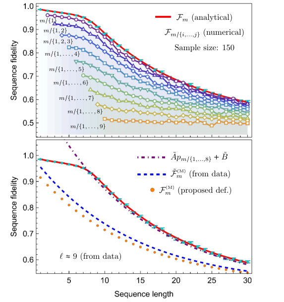
Henceforth we assume that an experimenter would not know both what the noise maps are, nor what the non-Markovian finite sequence length is. Given Corollary 1, however, we know that whenever we have finite time-independent non-Markovian noise, within the Markovian part the decay will be practically exponential with the non-Markovian part acting as SPAM errors. Specifically, here we would get an ASF of the form of Eq. (18) for almost time-independent noise (i.e. with almost equal noise-strengths ) after such sequence length . Our expression assumes that the transition to Markovian noise occurs from step to step, however, even if dissipation occurs smoothly and non-Markovianity never entirely fades, we can still estimate at which sequence length the memory of the noise stops being relevant by identifying exponential decays. This also allows to identify a Markovianized time-independent ASF with which the experimenter can estimate the impact of non-Markovian errors.
A way to achieve this in practice is by fixing Clifford gates to identity wherever the decay appears non-exponential; this will give an exponential decay of the ASF whenever there is at most one random Clifford within the non-Markovian sequence. In Fig. 6 we display the ASF, , both analytical and numerical, for a finite noise memory process with noise modeled by Eq. (25), again taking and . We also display numerical ASFs, denoted , with fixed identities at sequence lengths . The corresponding ASFs will normally be decreasing as given that fixing identities at subsequent steps is equivalent to set compounding error over such steps, which can be thought of simply as leaving the noise as a dynamical process to accumulate in time.
The non-Markovian sequence length can be identified by matching approximately the decay rate of one of these sequences with the corresponding one of the manifestly Markovian part in the full sequence. Once the decay rate has been determined, a sensible time-independent Markovianized ASF, , can be constructed by making reasonable assumptions for the SPAM factors and . Detail of this process is shown in Appendix G. For the case of the RB experiments in Fig. 6, the non-Markovian noise sequence length was determined to be by approximately matching with the corresponding one for the exponential fit between sequence lengths of the original data. Notice that in our model in Eq.(25), at sequence length the noise still has half probability of acting jointly on ; the found just says that after such sequence length the decay turns mostly exponential. We then finally constructed a Markovianized ASF with with supposing SPAM errors to be small; we compared this with a Markovianized construction as proposed in Section V, with time-independent noise given throughout by .
This practical approach can work reasonably well, as we show in this example, and allow both to determine the amount of memory within the noise, i.e, for how long the noise is being meaningfully non-Markovian, as well as to operationally construct a time-independent Markovianized ASF with which the impact of non-Markovianity in the noise can be quantified. The approach is consistent as well, in the sense that applying it to an exponential decay yields and at most a numerical error due to fixing an identity on the first step.
There are, however, two apparent downsides to this approach, one is having to run another set of experiments requiring a higher amount of samples, given that the noise accumulates and makes it harder to get reliable data, and the second is that the ASFs with fixed identities can eventually get too low if the noise memory is too high and not provide useful information. These are issues that could be resolved easily or otherwise depending on the particular case at hand.
Finally, while this approach cannot be used generally on fully non-Markovian noise, i.e. one over all sequence lengths, to determine operationally a sensible Markovianized ASF , it can nevertheless tell us whether the non-Markovian noise we are dealing with is coherent. This is important because whenever coherent noise can be diagnosed and characterized, e.g. with via unitarity measures Roth et al. 2018; Wallman et al. 2015; Dirkse et al. 2019; Girling et al. 2021 or otherwise, in principle it could be addressed and calibrated if we have access to the qubits. Precisely then, we may tell if the noise is unitary over the whole if we get a general non-exponential behavior described by Eq. (7) no matter how many identities we fix, or if some dissipation is occurring and we rather have a scenario closer to that of Corollary 3 of finite non-Markovian blocks of noise. We use the model of the previous section in Eq. (24) to exemplify this, as shown in Fig. 7. The way we can proceed is to run RB experiments with a given number of identities interleaved; if the deviations from an exponential disappear, or fade considerably, this might point out to some dissipation, otherwise we would be able to identify the noise as highly coherent. Here once again the challenge is rather with numerical precision and compounded error, as interleaving identities highly degrades the ASF.
IX Conclusions and Discussion
We have, i) derived a general analytical expression for the average sequence fidelity (ASF) of a randomized benchmarking (RB) experiment with the Clifford group subject to gate-independent non-Markovian noise, ii) proposed a theoretical measure to quantify non-Markovian deviations in an ASF, iii) derived the ASF for the case of finite non-Markovian noise, allowing to operationally estimate both non-Markovian noise time scales and the measure of deviations from Markovianity, and iv) exemplified all these with two proof of principle numerical examples. Along the manuscript we also discuss the effect of state preparation and measurement (SPAM) errors in RB with non-Markovian noise, as well as the case of classical correlations, which we argue can be treated as a Markovian time-dependent problem, and more generally the idea of RB blindness to a subclass of non-Markovian noise processes.
The ASF in our main result makes the depolarizing effect of averaging over Clifford gates on the system of interest manifest, while taking all of the noise in the sequence to the environment. The reduction of our main result to the standard Markovian gate-independent scenario is then straightforward with the trace over the environment giving rise to the noise strength and the SPAM error constants, and similarly one may consider cases where non-Markovian noise is finite over a subset of sequence lengths. Our main result also makes it clear that in general, non-Markovian noise will display non-exponential behavior, although we point out that there could be a subclass of non-Markovian models that do display an almost exponential decay that in practice would be almost impossible to resolve. We exemplified numerically how for small sequence lengths, deviations from Markovianity can be observed efficiently, as well as how the relevant time-frames for finite non-Markovianity can be operationally determined and non-Markovian deviations in the ASF quantified.
We highlight as well that the methods to quantify non-Markovian effects, determine memory time scales, and diagnose coherence of non-Markovian noise, could be implemented beyond the randomized benchmarking framework on other noise benchmarking, characterization or mitigation approaches whenever temporal correlations should be taken into account, e.g. for cross-talk or leakage errors Brown and Brown 2019; Strikis et al. 2020; Parrado-Rodríguez et al. 2021, similar to how it is done within the framework of resource theories in Ref. Berk et al. 2021 with the notion of temporal coarse-graining.
Needless to say, there are countless ways to move forward in the study of time-correlated errors in quantum computing. Arguably, the clearest ones arising from our manuscript within the RB procedure, would be to have a model-independent ASF, similar to the Markovian case, to benchmark other experimentally relevant groups or more generally arbitrary gate sets, to study context-dependent errors, with one possible way being the one we propose in Fig. 8, or to incorporate non-Markovianity in the general RB framework carefully constructed in Ref. Helsen et al. 2020. All of these extensions have already been studied in quite some depth for Markovian errors and doing the same for the non-Markovian case would be a natural step forward. Other than this, there are questions that still would need to be understood such as the impact of non-Markovianity in decay rates as a function of sequence length, or explicitly how a higher or lower amount of non-Markovianity affects the average gate fidelity. More generally, there is still a need to deeply understand errors arising from temporal correlations, and our result represents a step in this direction.
Acknowledgements.
We thank Felix A. Pollock for conversations. KM is supported through Australian Research Council Future Fellowship FT160100073 and Discovery Project grant DP210100597. KM was a recipient of the International Quantum U Tech Accelerator award by the US Air Force Research Laboratory. RH is supported by the Australian Research Council Centre of Excellence for Engineered Quantum Systems (Grant No. CE 170100009).References
- Emerson et al. (2005) J. Emerson, R. Alicki, and K. Życzkowski, Scalable noise estimation with random unitary operators, J. Opt. B-Quantum S.O. 7, S347 (2005).
- Lévi et al. (2007) B. Lévi, C. C. López, J. Emerson, and D. G. Cory, Efficient error characterization in quantum information processing, Phys. Rev. A 75, 022314 (2007).
- Knill et al. (2008) E. Knill, D. Leibfried, R. Reichle, J. Britton, R. B. Blakestad, J. D. Jost, C. Langer, R. Ozeri, S. Seidelin, and D. J. Wineland, Randomized benchmarking of quantum gates, Phys. Rev. A 77, 012307 (2008).
- Magesan et al. (2011) E. Magesan, J. M. Gambetta, and J. Emerson, Scalable and robust randomized benchmarking of quantum processes, Phys. Rev. Lett. 106, 180504 (2011).
- Magesan et al. (2012a) E. Magesan, J. M. Gambetta, and J. Emerson, Characterizing quantum gates via randomized benchmarking, Phys. Rev. A 85, 042311 (2012a).
- Helsen et al. (2020) J. Helsen, I. Roth, E. Onorati, A. H. Werner, and J. Eisert, A general framework for randomized benchmarking (2020), arXiv:2010.07974 [quant-ph] .
- Chuang and Nielsen (1997) I. L. Chuang and M. A. Nielsen, Prescription for experimental determination of the dynamics of a quantum black box, J. Mod. Optic 44, 2455–2467 (1997).
- Roth et al. (2018) I. Roth, R. Kueng, S. Kimmel, Y.-K. Liu, D. Gross, J. Eisert, and M. Kliesch, Recovering quantum gates from few average gate fidelities, Phys. Rev. Lett. 121, 170502 (2018).
- Wallman and Flammia (2014) J. J. Wallman and S. T. Flammia, Randomized benchmarking with confidence, New J. Phys. 16, 103032 (2014).
- Mohseni et al. (2008) M. Mohseni, A. T. Rezakhani, and D. A. Lidar, Quantum-process tomography: Resource analysis of different strategies, Phys. Rev. A 77, 032322 (2008).
- Nielsen et al. (2020) E. Nielsen, J. K. Gamble, K. Rudinger, T. Scholten, K. Young, and R. Blume-Kohout, Gate set tomography (2020), arXiv:2009.07301 [quant-ph] .
- Gross et al. (2010) D. Gross, Y.-K. Liu, S. T. Flammia, S. Becker, and J. Eisert, Quantum state tomography via compressed sensing, Phys. Rev. Lett. 105, 150401 (2010).
- Flammia et al. (2012) S. T. Flammia, D. Gross, Y.-K. Liu, and J. Eisert, Quantum tomography via compressed sensing: error bounds, sample complexity and efficient estimators, New J. Phys. 14, 095022 (2012).
- Flammia and Liu (2011) S. T. Flammia and Y.-K. Liu, Direct fidelity estimation from few pauli measurements, Phys. Rev. Lett. 106, 230501 (2011).
- da Silva et al. (2011) M. P. da Silva, O. Landon-Cardinal, and D. Poulin, Practical characterization of quantum devices without tomography, Phys. Rev. Lett. 107, 210404 (2011).
- Moussa et al. (2012) O. Moussa, M. P. da Silva, C. A. Ryan, and R. Laflamme, Practical experimental certification of computational quantum gates using a twirling procedure, Phys. Rev. Lett. 109, 070504 (2012).
- (17) In Ref. Proctor et al. 2017, it was pointed out that this relation between the ASF and the gate fidelity of the noise is not unique due to gauge invariance. An in-depth discussion can be seen in Ref. Wallman 2018; Merkel et al. 2018 with an overview and generalisation in Helsen et al. 2020.
- Proctor et al. (2017) T. Proctor, K. Rudinger, K. Young, M. Sarovar, and R. Blume-Kohout, What randomized benchmarking actually measures, Phys. Rev. Lett. 119, 130502 (2017).
- Wallman (2018) J. J. Wallman, Randomized benchmarking with gate-dependent noise, Quantum 2, 47 (2018).
- Helsen et al. (2019) J. Helsen, X. Xue, L. M. K. Vandersypen, and S. Wehner, A new class of efficient randomized benchmarking protocols, npj Quantum Information 5, 71 (2019).
- Carignan-Dugas et al. (2015) A. Carignan-Dugas, J. J. Wallman, and J. Emerson, Characterizing universal gate sets via dihedral benchmarking, Phys. Rev. A 92, 060302 (2015).
- Hashagen et al. (2018) A. K. Hashagen, S. T. Flammia, D. Gross, and J. J. Wallman, Real randomized benchmarking, Quantum 2, 85 (2018).
- Magesan et al. (2012b) E. Magesan, J. M. Gambetta, B. R. Johnson, C. A. Ryan, J. M. Chow, S. T. Merkel, M. P. da Silva, G. A. Keefe, M. B. Rothwell, T. A. Ohki, M. B. Ketchen, and M. Steffen, Efficient measurement of quantum gate error by interleaved randomized benchmarking, Phys. Rev. Lett. 109, 080505 (2012b).
- Wallman et al. (2015) J. Wallman, C. Granade, R. Harper, and S. T. Flammia, Estimating the coherence of noise, New J. Phys. 17, 113020 (2015).
- Ryan et al. (2009) C. A. Ryan, M. Laforest, and R. Laflamme, Randomized benchmarking of single- and multi-qubit control in liquid-state NMR quantum information processing, New Journal of Physics 11, 013034 (2009).
- Park et al. (2016) D. K. Park, G. Feng, R. Rahimi, J. Baugh, and R. Laflamme, Randomized benchmarking of quantum gates implemented by electron spin resonance, J. Magn. Reson. 267, 68 (2016).
- Epstein et al. (2014) J. M. Epstein, A. W. Cross, E. Magesan, and J. M. Gambetta, Investigating the limits of randomized benchmarking protocols, Phys. Rev. A 89, 062321 (2014).
- Fogarty et al. (2015) M. A. Fogarty, M. Veldhorst, R. Harper, C. H. Yang, S. D. Bartlett, S. T. Flammia, and A. S. Dzurak, Nonexponential fidelity decay in randomized benchmarking with low-frequency noise, Phys. Rev. A 92, 022326 (2015).
- Mavadia et al. (2018) S. Mavadia, C. L. Edmunds, C. Hempel, H. Ball, F. Roy, T. M. Stace, and M. J. Biercuk, Experimental quantum verification in the presence of temporally correlated noise, npj Quantum Inf. 4, 7 (2018).
- Ball et al. (2016) H. Ball, T. M. Stace, S. T. Flammia, and M. J. Biercuk, Effect of noise correlations on randomized benchmarking, Phys. Rev. A 93, 022303 (2016).
- Fong and Merkel (2017) B. H. Fong and S. T. Merkel, Randomized benchmarking, correlated noise, and ising models (2017), arXiv:1703.09747 [quant-ph] .
- Qi and Ng (2021) J. Qi and H. K. Ng, Randomized benchmarking in the presence of time-correlated dephasing noise, Phys. Rev. A 103, 022607 (2021).
- Gambetta et al. (2012) J. M. Gambetta, A. D. Córcoles, S. T. Merkel, B. R. Johnson, J. A. Smolin, J. M. Chow, C. A. Ryan, C. Rigetti, S. Poletto, T. A. Ohki, M. B. Ketchen, and M. Steffen, Characterization of addressability by simultaneous randomized benchmarking, Phys. Rev. Lett. 109, 240504 (2012).
- Milz and Modi (2021) S. Milz and K. Modi, Quantum stochastic processes and quantum non-markovian phenomena, PRX Quantum 2, 030201 (2021).
- Chiribella et al. (2008) G. Chiribella, G. M. D’Ariano, and P. Perinotti, Quantum circuit architecture, Phys. Rev. Lett. 101, 060401 (2008).
- Chiribella et al. (2009) G. Chiribella, G. M. D’Ariano, and P. Perinotti, Theoretical framework for quantum networks, Phys. Rev. A 80, 022339 (2009).
- Costa and Shrapnel (2016) F. Costa and S. Shrapnel, Quantum causal modelling, New J. Phys. 18, 063032 (2016).
- Pollock et al. (2018a) F. A. Pollock, C. Rodríguez-Rosario, T. Frauenheim, M. Paternostro, and K. Modi, Operational markov condition for quantum processes, Phys. Rev. Lett. 120, 040405 (2018a).
- Pollock et al. (2018b) F. A. Pollock, C. Rodríguez-Rosario, T. Frauenheim, M. Paternostro, and K. Modi, Non-markovian quantum processes: Complete framework and efficient characterization, Phys. Rev. A 97, 012127 (2018b).
- Gottesman (1997) D. Gottesman, Stabilizer codes and quantum error correction (1997), arXiv:quant-ph/9705052 [quant-ph] .
- Gottesman (1998) D. Gottesman, The heisenberg representation of quantum computers (1998), arXiv:quant-ph/9807006 [quant-ph] .
- Aaronson and Gottesman (2004) S. Aaronson and D. Gottesman, Improved simulation of stabilizer circuits, Phys. Rev. A 70, 052328 (2004).
- Dankert et al. (2009) C. Dankert, R. Cleve, J. Emerson, and E. Livine, Exact and approximate unitary 2-designs and their application to fidelity estimation, Phys. Rev. A 80, 012304 (2009).
- Nakata et al. (2021) Y. Nakata, D. Zhao, T. Okuda, E. Bannai, Y. Suzuki, S. Tamiya, K. Heya, Z. Yan, K. Zuo, S. Tamate, Y. Tabuchi, and Y. Nakamura, Quantum circuits for exact unitary -designs and applications to higher-order randomized benchmarking (2021), arXiv:2102.12617 [quant-ph] .
- Taranto (2020) P. Taranto, Memory effects in quantum processes, Int. J. Quantum Inf. 18, 1941002 (2020).
- Milz et al. (2017) S. Milz, F. A. Pollock, and K. Modi, An introduction to operational quantum dynamics, Open Syst. Inf. Dyn. 24, 1740016 (2017).
- Watrous (2018) J. Watrous, The Theory of Quantum Information (Cambridge University Press, 2018).
- (48) Strictly speaking, here we are defining , where is the Choi state of the sequence of gates , and can be defined to act on either auxiliary space or , the choice only depends on what auxiliary space the swap on the definition of swaps with, so that the contraction contracts the correct spaces.
- Milz et al. (2020) S. Milz, F. Sakuldee, F. A. Pollock, and K. Modi, Kolmogorov extension theorem for (quantum) causal modelling and general probabilistic theories, Quantum 4, 255 (2020).
- Nurdin and Gough (2021) H. I. Nurdin and J. E. Gough, From the Heisenberg to the Schrödinger picture: Quantum stochastic processes and process tensors (2021), arXiv:2109.09256 [quant-ph] .
- Milz et al. (2019) S. Milz, M. S. Kim, F. A. Pollock, and K. Modi, Completely positive divisibility does not mean markovianity, Phys. Rev. Lett. 123, 040401 (2019).
- Figueroa-Romero et al. (2019) P. Figueroa-Romero, K. Modi, and F. A. Pollock, Almost Markovian processes from closed dynamics, Quantum 3, 136 (2019).
- Figueroa-Romero et al. (2021) P. Figueroa-Romero, F. A. Pollock, and K. Modi, Markovianization with approximate unitary designs, Commun. Phys. 4, 127 (2021).
- (54) The action of the map can alternatively be written as with the Kraus operators of .
- Modi (2012) K. Modi, Operational approach to open dynamics and quantifying initial correlations, Sci. Rep. 2, 581 (2012).
- Ringbauer et al. (2015) M. Ringbauer, C. J. Wood, K. Modi, A. Gilchrist, A. G. White, and A. Fedrizzi, Characterizing quantum dynamics with initial system-environment correlations, Phys. Rev. Lett. 114, 090402 (2015).
- Rudinger et al. (2019) K. Rudinger, T. Proctor, D. Langharst, M. Sarovar, K. Young, and R. Blume-Kohout, Probing context-dependent errors in quantum processors, Phys. Rev. X 9, 021045 (2019).
- Giarmatzi and Costa (2021) C. Giarmatzi and F. Costa, Witnessing quantum memory in non-markovian processes, Quantum 5, 440 (2021).
- Milz et al. (2021) S. Milz, C. Spee, Z.-P. Xu, F. A. Pollock, K. Modi, and O. Gühne, Genuine Multipartite Entanglement in Time, SciPost Phys. 10, 141 (2021).
- Arenz et al. (2015) C. Arenz, R. Hillier, M. Fraas, and D. Burgarth, Distinguishing decoherence from alternative quantum theories by dynamical decoupling, Phys. Rev. A 92, 022102 (2015).
- Arenz et al. (2018) C. Arenz, D. Burgarth, P. Facchi, and R. Hillier, Dynamical decoupling of unbounded hamiltonians, J. Math. Phys. 59, 032203 (2018).
- Taranto et al. (2019a) P. Taranto, F. A. Pollock, and K. Modi, Memory strength and recoverability of non-markovian quantum stochastic processes (2019a), arXiv:1907.12583 [quant-ph] .
- (63) This observation can be seen to follow e.g. because we may upper-bound the total RB non-Markovianity of a sequence length experiment, in Eq. (15), as , where is general non-Markovianity for each intermediate step up to as in Eq. (5) with being a Schatten -norm, .
- Taranto et al. (2019b) P. Taranto, F. A. Pollock, S. Milz, M. Tomamichel, and K. Modi, Quantum markov order, Phys. Rev. Lett. 122, 140401 (2019b).
- Taranto et al. (2019c) P. Taranto, S. Milz, F. A. Pollock, and K. Modi, Structure of quantum stochastic processes with finite markov order, Phys. Rev. A 99, 042108 (2019c).
- White et al. (2021) G. A. L. White, F. A. Pollock, L. C. L. Hollenberg, K. Modi, and C. D. Hill, Non-markovian quantum process tomography (2021), arXiv:2106.11722 [quant-ph] .
- Heinz and Burkard (2021) I. Heinz and G. Burkard, Crosstalk analysis for single-qubit and two-qubit gates in spin qubit arrays (2021), arXiv:2105.10221 [cond-mat.mes-hall] .
- Tamascelli et al. (2018) D. Tamascelli, A. Smirne, S. F. Huelga, and M. B. Plenio, Nonperturbative treatment of non-markovian dynamics of open quantum systems, Phys. Rev. Lett. 120, 030402 (2018).
- Luchnikov et al. (2019) I. A. Luchnikov, S. V. Vintskevich, H. Ouerdane, and S. N. Filippov, Simulation complexity of open quantum dynamics: Connection with tensor networks, Phys. Rev. Lett. 122, 160401 (2019).
- Dirkse et al. (2019) B. Dirkse, J. Helsen, and S. Wehner, Efficient unitarity randomized benchmarking of few-qubit clifford gates, Phys. Rev. A 99, 012315 (2019).
- Girling et al. (2021) M. Girling, C. Cirstoiu, and D. Jennings, Estimation of correlations and non-separability in quantum channels via unitarity benchmarking (2021), arXiv:2104.04352 [quant-ph] .
- Brown and Brown (2019) N. C. Brown and K. R. Brown, Leakage mitigation for quantum error correction using a mixed qubit scheme, Phys. Rev. A 100, 032325 (2019).
- Strikis et al. (2020) A. Strikis, D. Qin, Y. Chen, S. C. Benjamin, and Y. Li, Learning-based quantum error mitigation (2020), arXiv:2005.07601 [quant-ph] .
- Parrado-Rodríguez et al. (2021) P. Parrado-Rodríguez, C. Ryan-Anderson, A. Bermudez, and M. Müller, Crosstalk Suppression for Fault-tolerant Quantum Error Correction with Trapped Ions, Quantum 5, 487 (2021).
- Berk et al. (2021) G. D. Berk, S. Milz, F. A. Pollock, and K. Modi, Extracting quantum dynamical resources: Consumption of non-markovianity for noise reduction (2021), arXiv:2110.02613 [quant-ph] .
- Merkel et al. (2018) S. T. Merkel, E. J. Pritchett, and B. H. Fong, Randomized benchmarking as convolution: Fourier analysis of gate dependent errors (2018), arXiv:1804.05951 [quant-ph] .
- Bengtsson and Życzkowski (2017) I. Bengtsson and K. Życzkowski, Geometry of Quantum States: An Introduction to Quantum Entanglement (Cambridge University Press, 2017).
- Figueroa-Romero (2021) P. Figueroa-Romero, Equilibration and typicality in quantum processes (2021), arXiv:2102.02289 [quant-ph] .
- Collins (2003) B. Collins, Moments and cumulants of polynomial random variables on unitary groups, the Itzykson-Zuber integral, and free probability, Int. Math. Res. Notices 2003, 953 (2003).
- Collins and Śniady (2006) B. Collins and P. Śniady, Integration with respect to the haar measure on unitary, orthogonal and symplectic group, Commun. Math. Phys. 264, 773–795 (2006).
Appendix A The process tensor of the noise and gate sequences
The process tensor is a multi-linear map taking CP maps as input and giving a single quantum state as output. The operational scenario is the following: an initial quantum state on the joint composite is acted on with an operation solely on system , which in general is given by a CP map; subsequently the whole composite evolves unitarily through a unitary map , after which an operation is performed on , then the whole evolves unitarily under a unitary map , and so on, until an intervention , followed finally by a unitary map . This means the final state in system will be given by
| (26) |
where here we implicitly write for . The process tensor is thus a map , where means space of bounded linear operators over the Hilbert space , taking CP maps as arguments and giving a quantum state as output at time-step , i.e.
| (27) |
where . Such operations are said to form an intervention and belong to an instrument, which can be understood as a generalization of a POVM, and the particular outcomes of each intervention yield a joint probability distribution describing a stochastic process.
The generalization of a Choi-state, as given by the Choi-Jamiołkowski isomorphism Watrous 2018; Bengtsson and Życzkowski 2017, for a -step process tensor follows by introducing maximally entangled states , where and similarly for , and letting half of each (that is, the part of either subspace or ) act as an input at every step by swapping the input spaces with the corresponding auxiliary space. This is more clearly illustrated in Fig. 9.
Specifically, the Choi-state of the process tensor takes the form
| (28) |
where here we are implicitly writing for and . The generalized swap between system and an auxiliary space at time-step is defined by , where here
| (29) |
Similar to the case of quantum channels, the isomorphism between the action of the process tensor and its Choi representation is manifest Figueroa-Romero 2021 through the relationship
| (30) |
where here
| (31) |
is the Choi-state for the operations , the notation stands for partial trace over all except output in , and denotes a transpose.
The tensor is an example of a Markovian process tensor in the sense that it does not have any temporal correlations and thus assumes a product form. For a Markovian dynamical -step process, , the Choi-states can either correspond to a closed system dynamics between steps and , or in general to a CP dynamics, e.g. that of an open system, where the environment is discarded between each step and no information passes on to the next step, as shown in Figure 10. The order of the spaces will be relevant whenever two tensors are contracted and can be written generally through swaps with auxiliary spaces and half maximally entangled states.
In this manuscript we describe a noise RB sequence as a process tensor with the dynamics being described by the noise at each step, . Explicitly, in the main text we denote the tensor Choi-state for a -step process for the noise as
| (32) |
where is an identity map on an auxiliary space composed of pairs of systems, is a swap gate between and one of these pairs in the th auxiliary space, say , and is an unnormalized maximally entangled state. The tensor state for the gate sequence, on the other hand, can be defined simply
| (33) |
where strictly speaking, here we are defining , where is the Choi state of the sequence of gates , and can be defined to act on either auxiliary space or , the choice only depends on what auxiliary space the swap on the definition of swaps with, so that the contraction contracts the correct spaces.
Appendix B Average gate sequence
Representing the noise and gate sequences as process tensors implies that computing the ASF just requires computing the average gate sequence, .
Whenever the gates entering this sequence belong to at least a unitary 2-design, we can simply replace the average over gates by that over unitaries distributed uniformly, i.e. according to the Haar measure, say , over the -dimensional unitary group, which we denote . The Haar measure is the unique measure on satisfying invariance under left and right multiplication, i.e. it is invariant under arbitrary rotations. Specifically, given a subset , we have for the Haar measure, , with the (left-right invariance) property
| (34) |
for any fixed . For any quantity depending on a unitary , we denote integration over such unitary by and refer to it as the Haar or uniform average of .
Let the action of the unitary maps be given by , then let us compute
| (35) |
where crucially, . This means that we need to be able to compute integrals with two pairs of and terms. One way to do this is by employing the 2-moment of , given by Collins 2003; Collins and Śniady 2006
| (36) |
where here the subindices refer to components of the same matrix (with denoting complex conjugate), with the extra subindices being mere labels, and where is the symmetric group on 2 elements. The symbol is the Weingarten function, which here takes the values
| (37) |
on the two possible permutations .
Then we can let for each and employ the 2-moment above; let us take the integral over first,
| (38) |
then we can do similarly with all remaining unitaries by also labeling each permutation mapping and for the corresponding integral over each , i.e.
| (39) |
where for easiness of notation we dropped the primes and denoted , where a sum is implicit over basis vectors and permutations on , and where stands for the usual Kronecker . We finally notice that .
Appendix C Average sequence fidelity
The Markovian case. As a first case let us verify that the average gate sequence given by Eq. 39 reproduces an ASF described by a decaying exponential in the number of gates when the noise is Markovian.
Consider first a single gate, . We have
| (40) |
where implicitly depends on , with each and being summed over the symmetric group , and with an implicit sum over each and .
For the Markovian process tensor, we consider noise described by some -dimensional CP map at time-step with Kraus representation , so that
| (41) |
Let us simply denote as , as there is no environment to care about. Then we obtain the average sequence
| (42) |
Now, if the noise is trace-preserving as well, we have . Then we get
| (43) |
where we define as a depolarising map with the so-called noise-strength,
| (44) |
which has to be constrained to . If we denote the noise map , with the Kraus operators acting on the respective system Hilbert space and conjugate space, resp., we can simply write
| (45) |
The noise-strength can be shown to be related to the gate fidelity of with respect to the identity Fogarty et al. 2015, i.e. , as . This is the relevant parameter which in practice can be recovered by running several sequences for different lengths and averaging the resulting probabilities.
To generalize to an arbitrary number of time-steps, we now use the fact that the action of the depolarizing channel can be written as
| (46) |
for any , which follows from Eq. (42). This then implies that for an arbitrary sequence length,
| (47) |
where here now , as expected. The case corresponds to the Markovian time-dependent noise case as in Ref. Wallman and Flammia 2014. When the noise-strengths are the same this gives the usual fitting model for the average probabilities
| (48) |
with and , which relate to state preparation and measurement errors.
General non-Markovian gate-independent noise. We now consider the general situation where the noise is correlated across each step through an external environment as depicted in Fig. 1. Let us take first the simplest case ; the process tensor for the noise sequence is
| (49) |
where here , hence we get
| (50) |
Let us write the Kraus operators of the th noise map, , as
| (51) |
where the and indices refer to systems and , resp.; the subindex is simply a label for the th Kraus operator. Then
| (52) |
and let us now similarly write the initial state as
| (53) |
then also
| (54) |
where the second line follows by Eq. (46) and by defining
| (55) |
Now let
| (56) |
so that
| (57) |
Now, we can also define
| (58) |
where summation is over all …and …, and which contains all information about the noise within the whole and the correlations in between the two. We can simply write this as as in the main text, where an identity on is implicit. With this we can write Eq. (54) as
| (59) |
In general, for an arbitrary sequence length, we have
| (60) |
so that,
| (61) |
The sequential application of maps is given by
| (62) |
where
| (63) |
and is a sum of all -term product combinations of and , that is,
| (64) | ||||
| (65) | ||||
| (66) | ||||
where and similarly for ; in general there are of these summands on . However, notice that as , every term simplifies to products of deltas, i.e.
| (67) |
This expression contains terms, and could potentially be useful whenever the underlying noise model is not known, as all this information will be contained solely on the factors .
We can, however, write this expression in a more succinct way. We have
| (71) |
so now let us define the following. Let
| (72) | ||||
| (73) |
for any operator acting on . Then we notice that
| (74) |
where as before there are implicit identities which should be clear by context, i.e. for example means . Then this means that
| (75) |
where . Now for the second term, similarly (again we omit implicit identity operators),
| (76) |
Appendix D Markovian limit
For the Markovian limit we take and . First, let us notice that, assuming are CPTP,
| (80) |
for any operators acting on and on . Then this implies that
| (81) |
where here as well is the noise-strength of , and
| (82) |
which implies that under Markovian noise.
Appendix E Finite non-Markovian noise
Initial non-Markovian noise. Suppose a quantum noise process is non-Markovian up to some time-step and almost Markovian in the remaining steps, i.e. , where is a Markov process from time-step to time-step . This effectively would mean that is traced at the th step and the remaining noise maps act only on . We can describe this by replacing the action of the noise map at the th-step as , where is the joint state at such step, and where is some fiducial state of . The remaining noise maps will be given by for with some CPTP maps . This implies that
| (83) |
and also . In particular if the final noise were trace-preserving, we would have . In general, however, this implies
| (84) |
where here again is the noise-strength corresponding to .
This means, as one would expect, that in such a case if non-Markovian noise cannot be resolved with an RB sequence length , it would amount to SPAM errors, with any subsequent ASF decay being Markovian. Notice however, that for short sequence lengths, non-Markovian noise could be resolved on average with a few runs of the RB protocol; as explained in the main text, this would allow to estimate the degree of non-Markovianity in the underlying process.
Late non-Markovian noise. Now consider the opposite, where the noise process is initially Markovian but somehow stops being superfluous after some time-step , i.e. . Now we have
| (85) |
where here we defined
| (86) |
whilst now , where similarly, . Thus
| (87) |
so we get a similar behavior, but in this case, as we have seen, it would generally be harder to resolve non-Markovian effects in RB if these occur at longer sequences.
Blocks of finite non-Markovian noise. Now we may consider the case when the noise process is split in two non-Markovian processes, i.e. the first noise process somehow approximately resets the environment at step and the remaining noise process is also non-Markovian until step , i.e. Now the only difference from a standard non-Markovian ASF is that at the th step we have , where again is some fiducial state of and is the state of at the th step. This means we can write
| (88) |
whilst now,
| (89) |
so we may write
| (90) |
This is a much more complicated behavior, but notice that similarly now after a sequence length , the first block of non-Markovian noise will be manifest only as SPAM errors. Also, now in essence any other possible mixture of Markovian and non-Markovian noise can be considered, e.g. if there is Markovian noise in-between this would give rise to factors within the first summand of Eq. (90) containing , and factors in the second summand.
In particular, suppose we have two blocks of finite non-Markovian noise, first one of length , and then a second block of length . Then we get a recursive expression for the ASF of the form
| (91) |
If moreover the initial state is uncorrelated, , we get
| (92) |
This then generalizes to blocks with finite non-Markovianity , where are sequence lengths.
Appendix F Classical non-Markovian noise
Classical dephasing noise. For the case of classical correlations we now exemplify how we may describe these through a classical memory specified by an external classical stochastic process whose outputs control the noise at every step . We can depict a circuit for the RB sequence as in Fig. 11(a). Here we focus on the model by Ref. Ball et al. 2016 and verify that we obtain the same behavior for the ASF.
In particular, such model takes a qubit system with errors where where and with is a random variable determined by the classical external control; such variables are randomly sampled but then fixed for the whole RB experiment. Thus a sequence of length can be treated as a Markovian time-dependent decay , where knowing the Kraus operators , we can compute for small
| (93) |
Letting the classical memory be a normally distributed discrete stochastic process with mean and variance , the so-called Markovian scenario considers the control operations at step giving a realization and setting . That is, all errors being independent of each other. Ignoring SPAM errors, suppose , so that
| (94) |
The other extreme scenario is when all noise random variables are identical so that , so-called DC-noise; here the control should measure a realization with probability and update the memory with a PDF of the form , where here is a Dirac delta distribution. Then , which similarly for becomes simply
| (95) |
For both extreme cases we see that we effectively reproduce the behavior described in Ball et al. 2016, in particular for the average sequence fidelity. Here we still have to average over the classical random variable:
| (96) |
For the Markovian case, the average can be carried out to obtain a decay , where here is the true error rate together with the classical noise. For a standard deviation of , this gives . The DC-case, as expected is more complicated, and one possibility is to expand the cosine function around to analyze the average fidelity, similar to how it is done in Ball et al. 2016 with contributions up to . The final behavior of differs both from an exponential and a simple product of noise-strengths. We show plots for the average fidelities in both cases with a standard deviation of in Fig. 11(b),11(c).
The shallow pocket model. We now consider a similar model for a qubit coupled to degree of freedom (d.o.f.) on a real line, which acts as an environment. This is labeled a shallow pocket model because such d.o.f. cannot store energy internally. This is an interesting model for several reasons, but here mainly because it leads to completely positive and divisible dynamics of but it is nevertheless non-Markovian Taranto et al. 2019a; Milz and Modi 2021. For RB, however, the nature of classical correlations is what leads to a treatment of the ASF as a time-dependent Markovian one.
The shallow pocket model now considers with , where is a position operator at time-step and are time-intervals representing evolution time of the th step. This immediately implies that the average sequence is of the form , where . The initial state of the environment d.o.f. is taken as such that . Now tracing out the environment at the end of the process is equivalent to integrating over the reals with a factor . Thus we can think of the external d.o.f. as a classical DC noise distributed with a probability density function .
That is, now we have
| (97) |
Notice that all ’s have to be constrained to , so to have a meaningful ASF the equivalent of our distribution, namely , has to contain a low enough equivalent of a variance, which amounts to choosing an appropriate value for . Hence, now taking and , we get
| (98) |
which is somewhat harder to evaluate given that expanding around small is not a viable option. Regardless, the point we make here is that classical correlations such as the one before of dephasing noise or the shallow pocket model can be treated on RB with a standard Markovian time-dependent approach.
Appendix G Numerical calculations
SPAM errors. As in the main text, here we consider a qubit subject to time-independent unitary noise on a full -qubit system, where with given by the -site Ising spin chain
| (99) |
with being Pauli matrices acting on the th site. We take a closed chain so that . In particular, in the main text we take only qubits, with site being system .
Here we pick the values , and , fixing . To take into account SPAM errors numerically, suppose the initial state is previously affected by the same error for some small , and that is slightly rotated via for a small . In Fig. 12 we show examples for both mild, and , and much worse, and . We also consider the case where the preparation affects only by some rotation with a small , but does not generate correlations with .
In all cases SPAM makes it harder to numerically resolve non-Markovian effects. Similar to the Markovian case, SPAM errors generate an offset of the ASF, but in general they also affect the decay rate of the errors. This can be argued to be mainly due to the correlating effect of errors but changes in the decay rates can also be seen when the preparation does not generate correlations with . The impact of SPAM in the characterization of non-Markovian noise with RB is thus an issue that still has to be studied in greater detail.
Absence of non-exponential behavior. We notice that for a similar noise model for a couple of qubits,
| (100) |
essentially no deviation from an exponential is seen. We look again at time-independent noise given by with small and take , where one of the qubits is identified as system and the other one as the environment , and take . We show the corresponding ASF in Fig. 13 for the arbitrary choices , .
Notice that small deviations do occur at very short sequence lengths, although they are practically negligible. While of course, we are not quantifying the non-Markovianity of the model, and also different choices of the couplings might display larger deviations, the point we want to make is that there are going to be models that are blind, or at least myopic, to non-Markovianity when employing RB, and the circumstances when this occurs are still to be better understood.
Increasing environment dimension. We now look at the effect of increasing the number of qubits in ; noticeably the environment dimension does not show up explicitly in the main ASF in Eq. (7). We now employ similar conditions on the Hamiltonian in Eq. (99) for a changing value of . In Fig. 14 we show the deviations from RB non-Markovianity for up to 5 environmental qubits, and notice that the non-exponential deviations get effectively damped, albeit slowly and for longer sequence lengths first. This is expected behavior, but nevertheless it is still a question what is exactly the dependence of the general non-Markovian ASF in environment dimension.
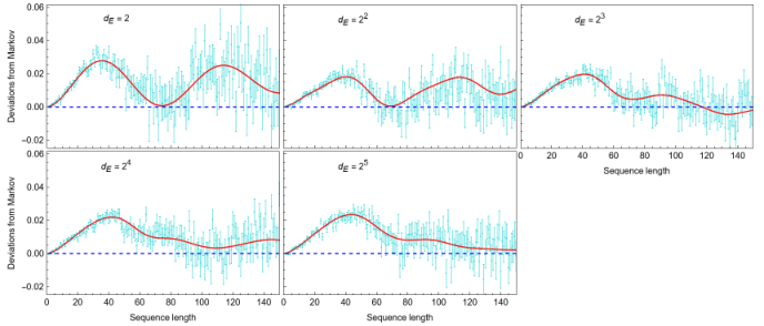
Finite non-Markovian sequence lengths and non-Markovian deviations. Whenever we have finite non-Markovian noise, say over an initial sequence length , described by the CP maps , and an uncorrelated input state, by choosing to fix Cliffords after the first one to be identities, by Eq. (84), we get a Markovian decay with , where
| (101) |
with
| (102) |
with each in terms of Kraus operators acting on spaces and co-spaces as .
That is, the initial block of finite non-Markovian noise looks like a single noise map if we randomize over a single Clifford within this block, with the remaining ones set to identities.
While this is an idealized scenario, we can use it to estimate sequence lengths at which non-Markovian noise effects are relevant in an RB experiment. In the main text we model such a noise process with a noise map at the th step given by
| (103) |
where here again with where is given by Eq. (99) and acts on as . In the main text we also fix the values , and and set , although we now pick a for . This implies that the noise acts jointly over the whole throughout the full process, but it acts almost fully as for , whilst it turns almost to act solely on with for .
In the top figure of Fig. 6 in the main text, we display the ASFs for a set of RB experiments with and for different sets of fixed identities at sequence lengths . We fix and we describe the way in which an experimenter can estimate this value of from the data of the experiments alone, as well as construct a sensible time-independent Markovian ASF with which they can quantify the amount of non-Markovian deviations; this is shown in the bottom panel of the same figure.
The procedure is the following given a single ASF, , displaying a non-exponential decay over a finite sequence length:
- 1.
Fix identities at sequence lengths of manifestly displaying deviations from an exponential decay and run RB experiments for each of them, obtaining corresponding ASFs , where are sequence lengths at which identities were fixed.
- 2.
Identify the section of the original manifestly displaying exponential behavior and extract the noise rate at such section.
- 3.
Fit an exponential to each ; Eq. (84) implies that the curve with an exponential rate closest to will indicate the length at which the noise turns almost Markovian (or where non-Markovian effects become negligible).
- 4.
Finally, a Markovianized ASF can be constructed with rate and at least two reasonable constraints for the SPAM constants, such as and if the SPAM errors are assumed low and the decay rate is not too high, .
For the particular example in the main text, step 1 is displayed in the top panel of Fig. 6, each over 150 samples.
For step 2, we took points from to , which more manifestly display an exponential decay. These were fitted to an exponential , i.e. we extract .
For step 3, we identified the closest decay rate to occurred for , with . This indicates that . Since we fixed , this procedure is essentially identifying that the non-Markovian effects of the noise on the ASF become negligible at sequence length ; notice that at this length , i.e. so that the noise will still act jointly on with at least half probability. In this sense is just approximated numerically. In the bottom panel of Fig. 6, the dot-dashed line displays the curve given by , showing the slight offset due to this numerical estimation.
Finally, at step 4 we simply fix in assuming low spam errors; in Fig. 6 we specifically take and with the demand that converges to the same value as in and for . As is the case for RB, this Markovianized ASF curve at most informs us about the gate fidelity with respect to the identity of the Markovianized noise through .