Fock State-enhanced Expressivity of Quantum Machine Learning ModelsPreprint: APS/123-QED
Abstract
The data-embedding process is one of the bottlenecks of quantum machine learning, potentially negating any quantum speedups. In light of this, more effective data-encoding strategies are necessary. We propose a photonic-based bosonic data-encoding scheme that embeds classical data points using fewer encoding layers and circumventing the need for nonlinear optical components by mapping the data points into the high-dimensional Fock space. The expressive power of the circuit can be controlled via the number of input photons. Our work shed some light on the unique advantages offered by quantum photonics on the expressive power of quantum machine learning models. By leveraging the photon-number dependent expressive power, we propose three different noisy intermediate-scale quantum-compatible binary classification methods with different scaling of required resources suitable for different supervised classification tasks.
I Introduction
Machine learning approaches such as artificial neural networks are powerful tools for solving a wide range of problems including image classification and regression. However, the scalability of machine learning implemented using general-purpose electronic circuits is limited by their high power consumption and the end of Moore’s law. These issues motivate the pursuit of dedicated hardware for machine learning including photonic neural networks De Marinis et al. 2019; Hamerly et al. 2019; Roques-Carmes et al. 2020; Shastri et al. 2021 and quantum circuits Peruzzo et al. 2014; Mitarai et al. 2018; Benedetti et al. 2019; Schuld et al. 2020; Fujii and Nakajima 2021; Goto et al. 2021; Lloyd et al. 2020.
The combination of ideas from the photonic and quantum machine learning communities may enable further speed-ups and novel functionalities Chatterjee and Yu 2016; Schuld and Killoran 2019; Steinbrecher et al. 2019; Killoran et al. 2019; Bartkiewicz et al. 2020; Taballione et al. 2021; Chabaud et al. 2021; Ghobadi 2021. For example, both classical and quantum photonic neural networks are presently limited by the difficulty of incorporating nonlinear activation functions. This challenge can be circumvented using the kernel trick, in which the input data is mapped into a high-dimensional feature space where simple linear models become effective Schuld and Killoran 2019; Havlíček et al. 2019; Schuld and Petruccione 2021; Schuld 2021. The simplest quantum feature map based on repeated application of data-dependent single qubit rotations is already sufficient to serve as a universal function approximator Pérez-Salinas et al. 2020; Schuld et al. 2021; Pérez-Salinas et al. 2021.
Despite progress in various aspects of near-term quantum machine learning algorithms Li and Deng 2022 including experimental realizations Bartkiewicz et al. 2020; Dutta et al. 2021; Kusumoto et al. 2021; Peters et al. 2021; Ren et al. 2022, proposals for various platforms Kusumoto et al. 2021; Tangpanitanon et al. 2020 and studies of statistical properties of quantum machine learning models Abbas et al. 2021; Holmes et al. 2022; Caro et al. 2021a, the encoding of input data is still a significant bottleneck for (quantum) photonic machine learning hardware. For example, the expressive power of quantum circuits based on parameterized single qubit rotations is limited by the number of encoding gates used Pérez-Salinas et al. 2020; Schuld et al. 2021. Similarly, some existing quantum machine learning algorithms with proven speedups for future fault-tolerant quantum computers assume the existence of quantum-random access memory (RAM) Giovannetti et al. 2008 that can provide the input data in a quantum superposition with no overhead Harrow et al. 2009; Wiebe et al. 2012; Lloyd et al. 2013; Lloyd et al. 2014; Rebentrost et al. 2014; Biamonte et al. 2017; Dunjko and Briegel 2018. Yet, the sources of the speedup of these algorithms are still under active debate Tang 2021; Cotler et al. 2021. Thus, a pressing goal is to develop machine learning algorithms that avoid encoding large input datasets Lloyd et al. 2016; Harrow 2020; Liu et al. 2021 or more efficient data-encoding methods. This article addresses the latter problem.

Specifically, we generalize the qubit-based circuit architecture analyzed in Refs. Pérez-Salinas et al. 2020; Schuld et al. 2021 to quantum photonic circuits (QPCs) constructed using linear optical components such as beam splitters and phase shifters, photon detectors, and Fock state inputs. We consider parameterized linear QPCs [Fig.1(a)] consisting of two trainable circuit blocks with one data encoding block sandwiched between them. We show that for a fixed number of encoding phase shifters, the expressive power of the parameterized quantum circuit is improved by embedding the classical data into the higher-dimensional Fock space. This enables the approximation of classical functions using fewer encoding layers while circumventing the need for nonlinear components. The origin of this improved encoding efficiency is that each phase shifter simultaneously uploads the input data onto multiple Fock basis states simultaneously.
Similar to Ref. Schuld et al. 2021, -photon quantum machine learning models can be expressed as a Fourier series
| (1) |
where is the frequency spectrum and are the Fourier coefficients that depend on trainable circuit block’s parameters and observable’s parameters . The expressive power of the Fourier series is determined by two components: the spectrum of frequencies , and the Fourier coefficients . We show that the frequency spectrum of the circuit can be controlled by the number of input photons. Thus, a rich frequency spectrum can be generated by providing sufficient number of input photons to linear QPCs with a constant number of spatial modes. In contrast, qubit-based circuits require deeper or wider circuits to increase the size of their frequency spectrum. When generalized to arbitrary input states and observables the QPCs can also generate arbitrary set of Fourier coefficients that combine the frequency dependent basis functions , allowing them to approximate any square-integrable function on a finite interval to arbitrary precision Carleson 1966; Weisz 2012; Schuld et al. 2021.
As an application of the parameterized linear quantum photonic circuits, we consider three different machine learning approaches for supervised data classification: (1) A variational classifier based on minimizing a cost function by training the circuit parameters. (2) Kernel methods, which employ fixed circuits, with training carried out on observables only. (3) Random kitchen sinks, which use a set of random circuits to approximate a desired kernel function. Each of these methods has different scaling with the dimension of the data and number of training points used, and so each is better-suited to different types of supervised learning problems.
The outline of this paper is as follows. Sec. II introduces our proposed linear quantum photonic circuit architecture and analyzes how its expressive power depends on the number of spatial modes and input photons. Next, Sec. III illustrates the photon number-dependent performance of the circuit for supervised classification problems. Sec. IV concludes the paper.
II Parametrized linear quantum photonic circuit model
To demonstrate the Fock state-enhanced expressive power of linear quantum photonic circuits, in this Section we consider the encoding of univariable functions onto circuit’s output. For simplicity we consider the circuit architecture illustrated schematically in Fig. 1, consisting of a single data-dependent encoding layer sandwiched between two trainable beam splitter meshes , described by the unitary transformation
| (2) |
where parameterizes transformations applied by trainable beam splitter meshes and is the input data. The -photon quantum model (circuit’s output) is defined as the expectation value of some observable with respect to a state prepared via the parameterised linear QPC,
| (3) |
where is the input -photon Fock state with and parameterizes the observable. We consider measurements made using either photon number-resolving (PNR) detectors or single photon (threshold) detectors, corresponding to being diagonal in the Fock state basis with or distinct parameterized eigenvalues , respectively.
The multi-mode Fock state unitary transformation is constructed from permanents of submatrices of the -mode linear transformation matrix using the scheme of Ref. Scheel 2004 with as the programmable transfer matrix, describing the universal multiport interferometer that realizes arbitrary linear optical input-output transformations Reck et al. 1994; Clements et al. 2016; Bell and Walmsley 2021. Each trainable unitary is parameterized by a vector of phase shifter and beam splitter angles constructed using the encoding of Reck et al. Reck et al. 1994. The data encoding block employs a single tunable phase shifter placed at the first spatial mode.
II.1 -photon quantum models as Fourier series
In this Section we will show how to express the -photon quantum models as a Fourier series. For simplicity, we consider arbitrary unitary operations , an arbitrary parameterized observable obtained using PNR detectors , and as the initial Fock state. The component of the output quantum state with photon numbers can be written as Schuld et al. 2021
| (4) |
where the summation runs over the basis of Fock states corresponding to different combinations of photons in the spatial modes. The data encoding block imposes a phase shift proportional to the number of photons in the first mode following the first beam splitter mesh.
The output of full model Eq. (3) is obtained by taking the modulus square of Eq. (4), multiplying by the corresponding observable weight, and then summing over all output Fock basis states. This yields an expression of the form
| (5) |
where contain the matrix elements from the unitaries and measurement’s observable ,
| (6) |
This expression can be simplified by grouping the basis function with the same frequency . This gives
| (7) |
where the coefficients are obtained by summing over all contributing to the same frequency
| (8) |
with and Eq. (7) is a real-value function, as it should be. The frequency spectrum contains all frequencies that are accessible to the -photon quantum model. For general trainable circuit blocks , measurement observable and -photon Fock state , the -photon quantum model reads
| (9) |

II.2 Expressive power and trainability of linear quantum photonic circuits
Since the -photon quantum model can be represented by a Fourier series, its expressive power can be studied via two properties: its frequency spectrum and Fourier coefficients. The former tells us which functions the quantum model has access to, while the latter determines how the accessible functions can be combined Schuld et al. 2021.
II.2.1 Photon-number dependent frequency spectrum
The frequency spectrum can be easily shown to be
| (10) |
which is solely determined by the number of photons fed into the circuit. It always contains the zero frequency, i.e. , while the non-zero frequencies occur in pairs, i.e. . This motivates us to define the size of the frequency spectrum as to quantify the number of independent non-zero frequencies the -photon quantum model has access to. In comparison to Ref. Schuld et al. 2021, where the size of frequency spectrum is determined by the spectrum of the data encoding Hamiltonian, here the size of the frequency spectrum can be increased by feeding more photons into the circuit, while keeping the number of spatial modes and encoding phase shifters constant.
This implies that -photon quantum models with more input photons can be more expressive, because they have access to more basis functions, and hence can learn Fourier series with higher frequencies. In the limit of , i.e. continuous variable quantum systems, -photon quantum models can support the frequency spectrum of a full Fourier series, in agreement with Ref. Schuld et al. 2021. For a fixed number of input photons, the frequency spectrum can be broadened further using multiple encoding phase shifters, either in parallel or sequentially Schuld et al. 2021; Pérez-Salinas et al. 2020 (see Appendix A for details).
As an example, we consider training a linear QPC with three spatial modes shown in Fig. 2(a) using a regularized squared loss cost function. The cost function is constructed using the measurement results and a training set of desired input/output pairs
| (11) |
that is variationally minimized over and to learn the function . Here, is the -photon quantum model in Eq. (9), while is the sum of squared observable parameters, forming a regularization term with weight . The regularization term has a two-fold role: it prevents model over-fits, and ensures that the model prediction is not based on output photon combinations that occur with very low probability. The latter is important for QPC-based machine learning models, because the number of measurements required to obtain all of the required expectation values scales with the number of spatial modes and photons.
We train the three mode linear QPC using the gradient-free algorithm in the NLopt nonlinear-optimization python package Johnson 2014, i.e. BOBYQA algorithm Powell 2009 to fit a degree three Fourier series with using input states of up to 3 photons. We consider input states for which each spatial mode contains at most one photon, i.e. , , or . Fig. 3(a) shows how the number of observable frequency components and hence the expressive power of the circuit grows with the number of input photons. Perfect fitting is achieved with three photons. In contrast, the frequency spectrum of similar qubit-based architectures cannot fit a degree two Fourier series using a single encoding block, requiring either a deeper or wider circuits with multiple encoding gates Pérez-Salinas et al. 2020; Schuld et al. 2021.

II.2.2 Trainability of Fourier coefficients
Even if the parametrized QPC can generate the frequency spectrum required to fit the desired function, this does not necessarily imply that the optimal Fourier coefficients are accessible Schuld et al. 2021; the linear circuits we consider cannot perform arbitrary Fock state transformations. However, we do not need to generate arbitrary Fock states and only require control over one real and complex Fourier coefficients . For input photons and taking , this requires at least real degrees of freedom.
Each trainable circuit blocks has controllable parameters Reck et al. 1994, while the number of controllable degrees of freedom of the parameterized observable depends on type of detector. For photon number resolving (PNR) detectors the number of degrees of freedom is
| (12) |
while threshold detectors have
| (13) |
degrees of freedom.
For a fixed number of spatial modes and photons, threshold detectors have fewer controllable degrees of freedom compared to PNR detectors, and hence their expressive power saturates beyond a certain number of input photons. For example, Fig. 3(b) illustrates the expressive power of a circuit with three spatial modes. Using threshold detectors the expressive power is only enhanced by increasing the number of photons up to nine; beyond this, the number of controllable degrees of freedom is less than . On the other hand, using PNR detectors the circuit may in principle be trained to fit arbitrarily large frequencies by increasing the number of input photons. Of course, in practice the range of frequencies accessible using a single encoding gate will be limited by sensitivity to losses, which grows exponentially with the photon number.
II.2.3 Universality of the linear quantum photonic circuit
It is well known that a Fourier series can approximate any square-integrable function on a finite interval to arbitrary precision Carleson 1966; Weisz 2012. Thus, expressing the -photon quantum model in term of a Fourier series allows us to demonstrate the universality of the quantum model by studying its ability to realise arbitrary Fourier series. Universality of a Fourier series is determined by two important ingredients: a sufficiently-broad frequency spectrum and arbitrary realizable Fourier coefficients. The analysis in Sec. II.2.1 implies that the frequency spectrum accessible by -photon quantum models asymptotically contains any integer frequency if enough input photons are used, satisfying one of the criteria to achieve universality.
To realize arbitrary set of Fourier coefficients, at least degrees of freedom in the linear QPC are required. Here, we consider a linear QPC with PNR detectors. The PNR detectors are used because the expressive power of threshold detectors saturated beyond some threshold number of photons. One of the unique advantages of photonic system is the exponentially growing dimension of the Fock space with number of spatial modes and photons. For a linear QPC with constant number of spatial modes , the dimension of the Fock space and scales in the order of , hence contributing of degrees of freedom. On the other hand, the degrees of freedom from the trainable circuit blocks scale with , which is negligible when . By exploiting this advantage, it can be seen that is always larger than as the size of the frequency spectrum and scale linearly with photon number, i.e. . This is a necessary condition for the -photon quantum model being able to realize arbitrary set of Fourier coefficients, which in the examples we consider also seems to be sufficient. More rigorously, following the arguments in Ref. Schuld et al. 2021 a universal function approximator may be obtained by generalizing our circuits to arbitrary (entangled) input states and observables by incorporating nonlinear elements into the circuits 11 1 The nonlinear optical elements enables the realization of two qubit entangling gates, while arbitrary single qubit rotations can be realized using linear optics such as beam splitter and phase shifters. By considering the dual-rail photonic qubit, our circuit could perform universal quantum computation, and the Fourier coefficients arguments follows from Ref.Schuld et al. 2021..
As an example, we consider a linear QPC with 3 spatial modes. In this case, Eq. (12) is reduced to
| (14) |
which is always larger than for , as shown in Fig. 3(b). Hence, the -photon quantum model with 3 spatial modes and a single phase shifter can act as a universal function approximator. In contrast, the qubit-type variational quantum circuits require deep or wide circuits and many encoding gates to ensure a rich frequency spectrum, and arbitrary global unitaries to realize arbitrary sets of Fourier coefficients Schuld et al. 2021.
II.2.4 Effect of noise on the expressive power of linear quantum photonic circuits
For noiseless linear quantum photonic circuits, we have shown that its expressive power will improve with the increasing number of photons and spatial modes. In this section, we will discuss the role of optical losses on the expressive power of linear quantum photonic ciruits. For real quantum photonic hardware, the optical loss sensitivity will grows exponentially with the circuit depth and number of input photons. The typical noise sources are (1) inefficient collection optics, (2) losses in the optical components due to absorption, scattering, or reflections from the surfaces, (3) inefficiency in the detection process due to using detectors with imperfect quantum efficiency, and they can be modelled using beam splitters Fox 2006. These noises will obviously affect the frequency spectrum, where the higher frequency term cannot be distinguished from the lower frequency term, hence reducing the size of the frequency spectrum. We anticipate the noises to have a minimum impact on the Fourier coefficients, as they depend only on the physical components such as linear optics in trainable blocks and the detectors. Therefore, the output observables can still be written as Fourier series, just with reduced expressivity. This will place a practical limit on the complexity of the QML models using this scheme, unless one can include some kind of error correction scheme. When the losses are low enough, the detectors should have a sufficiently high signal to noise ratio that other noise sources can be neglected. Apart from the error correction scheme, the regularization term in the cost function should be able to help to minimize the detrimental influence of noise. It penalizes models including coefficients with huge weights, hence no particular output state should have a huge weight, reducing the model’s sensitivity of noise in final prediction. Finally, the photonic circuit considered here are based on variational approach, therefore, they are robust against variations in the beam splitter ratios, tuning, and etc. The quantitative noise modelling of the linear photonic quantum circuits will be a subject for future research.
III Supervised Learning using linear quantum photonic circuits

As an application of the trainable linear QPCs we now consider different strategies for binary classification. In the first strategy the linear QPCs are directly used as variational quantum classifiers, classifying data directly on the high-dimensional Fock space by optimizing a regularized squared loss cost function. In this case, as the circuit becomes more expressive it becomes harder to train. Second, we consider kernel methods as a means of avoiding the costly circuit optimization step. We show how linear circuits can be used to implement Gaussian kernels either directly or using the random kitchen sinks algorithm, sampling kernels with different resolutions in parallel. Note that we are mainly interested in what kinds of kernel functions can be efficiently implemented using linear QPCs, instead of providing quantum kernels that might offer quantum advantages, motivated by ongoing interest in classical photonic circuits for machine learning De Marinis et al. 2019; Hamerly et al. 2019; Roques-Carmes et al. 2020; Shastri et al. 2021.
III.1 Linear quantum photonic circuit as variational quantum classifiers
We perform binary classification of two-dimensional classical data. Each data dimension is encoded using a single phase shifter, as shown in Fig. 2(a). The mapping of the data into the high-dimensional Fock space is nonlinear, circumventing the need for nonlinear optical elements.
The -photon supervised classification model for two-dimensional data is defined as
| (15) |
where is the 2-dimensional data feature, is the 2-dimensional frequency vector, and , is the frequency spectrum of the model. This encoding scheme will not generate a full frequency spectrum for multi-dimensional Fourier series but it suffice for the example considered here. See Appendix B for schemes that generate full frequency spectrum for multi-dimensional Fourier series.
The model is trained by minimizing the cost function
| (16) |
using the BOBYQA algorithm, with the decision boundary defined as
| (17) |
where and are the optimized circuit’s and observable’s parameters and is the sign function. Thus, the class of the data points is assigned by the sign of circuit output.
As an example, we trained the linear QPC to classify three different types of datasets from the scikit-learn machine learning library Pedregosa et al. 2011: linear, circle, and moon. Fig. 4 illustrates the trained models. The contour plots show that -photon supervised classification models with higher photon number have more complicated classification boundaries, in agreement with previous analysis on the expressive power of quantum models. Since the linear data set can be separated by a linear decision boundary, unsurprisingly a single model photon is sufficient to learn the classification boundary. On the other hand, overfitting can occur when the model expressive power is too large, as can be seen for the degraded performance for the circle dataset for the input state. The classification performance for the more complicated moon dataset improves with the number of input photons. These examples illustrate the impact of a higher expressive power on classification using linear QPCs.
III.2 Linear quantum photonic circuits as Gaussian kernel samplers
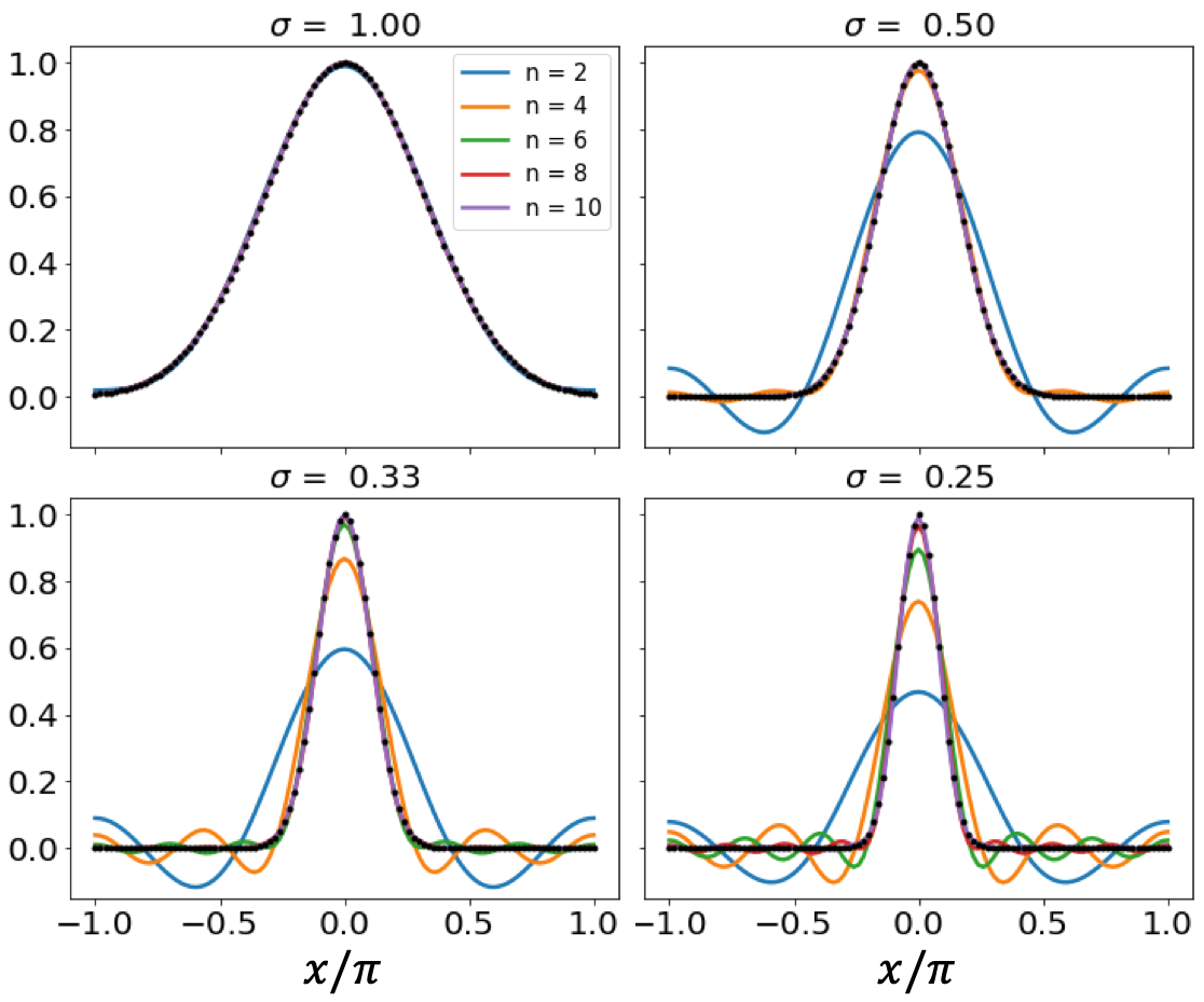
Similar to the standard noisy and large scale variational circuits, the variational machine learning approach becomes more difficult to train as the dimension of the Fock space increases, likely due to the issue of vanishing cost function gradients McClean et al. 2018; Wang et al. 2021a; Marrero et al. 2021; Bittel and Kliesch 2021; Thanasilp et al. 2021, requiring exponentially-growing precision to optimize the circuit parameters in-situ Arrasmith et al. 2021. In addition, it is expensive to train the quantum gates (in this case the tunable beam splitter meshes) in the noisy-intermediate scale quantum (NISQ) era as it is time-consuming to reprogram quantum circuits Harrow 2020. Due to these limitations, it is more efficient to use NISQ devices as sub-routines for machine learning algorithms, e.g. to sample quantities that are useful for classical machine learning models but time-consuming to compute. In particular, variational quantum circuits can be used to approximate kernel functions for classical kernel models such as support vector machines Bartkiewicz et al. 2020; Schuld and Killoran 2019; Havlíček et al. 2019; Goto et al. 2021; Haug et al. 2021. Here, we show how the linear QPCs can be designed to approximate Gaussian kernels with a range of resolutions determined by the number of input photons.
III.2.1 Kernel methods
Kernel methods allow one to apply linear classification algorithms to datasets with nonlinear decision boundaries Schölkopf and Smola 2002; Hofmann et al. 2008. The idea is to leverage feature maps that map the nonlinear dataset from its original space into a higher dimensional feauture space in which a linear decision boundary can be found, enabling classification via a linear regression
using suitably-trained weights . Instead of computing and storing the high-dimensional feature vector , the kernel trick Mercer 1909; Hofmann et al. 2008 is employed by introducing a kernel function , which measures the pairwise similarity between the data points in the feature space. Formally, the kernel functions is defined as the inner product of two feature vectors
| (18) |
According to representer theorem Schölkopf et al. 2001, the solution to the decision boundary can then be expressed in term of the kernel functions as
| (19) |
converting the optimization problem into a convex optimization problem of finding the parameters . In the case of a regularized squared loss cost function such as Eq. (16) the optimal parameters can be obtained analytically Bishop 2006; Theodoridis 2015 as
| (20) |
where is the number of training data, is the kernel matrix with matrix elements , is the -dimensional identity matrix, is the regularization parameter, and is the vector of the training data labels.
Although we currently have an example that shows rigorous performance guarantees of quantum kernel methods on artificial dataset Liu et al. 2021, it is still unclear whether quantum machine learning models can achieve improved performance compared to classical machine learning approaches in practical problems by sampling from kernels that are hard to compute classically Schuld and Killoran 2019; Schuld and Petruccione 2021; Huang et al. 2021; Wang et al. 2021b. Even in the absence of a rigorous quantum advantage, special-purpose electronic and photonic machine learning circuits are being pursued in order to increase the speed and energy-efficiency of well-established classical machine learning models De Marinis et al. 2019; Hamerly et al. 2019; Roques-Carmes et al. 2020; Shastri et al. 2021. Therefore, here we will focus on implementing the widely-used Gaussian kernel
with controllable resolution . The Gaussian kernel is a universal, infinite-dimensional kernel that can learn any continuous function in a compact space Micchelli et al. 2006.
III.2.2 Linear quantum photonic circuits as sub-routine of kernel methods
We approximate the Gaussian kernel using the two mode QPC shown in Fig. 2(b), where 50-50 beamsplitters are used for both trainable circuit blocks and the squared Euclidean distance between pairs of data points is encoded using a single phase shifter. The output of this circuit can be written as
where and the trainable observable with . Similar to Sec. III.1, the observable is trained to approximate the Gaussian kernel of resolution by minimizing the squared loss cost function using the BOBYQA algorithm
This approach has two advantages: Different kernel resolutions can be accessed using the same photon detection statistics by taking different linear combinations of the output observables . Second, this training only needs to be performed once; the tunable circuit blocks do not need to be reconfigured if the training data set changes.
We note that the domain of the input data, in this case the norm squared distances between pairs of data points, must lie within the interval that defines the circuit’s Fourier series. This imposes an upper bound on the kernel resolution that the linear QPC has access to. The circuit with higher expressive power, i.e. higher number of input photons, can more precisely approximate kernels with higher resolution . Kernels with lower resolution can already be well-approximated by a circuit with only two input photons. Fig. 5 shows the kernel training result for different desired resolutions and input photon numbers. Once the kernel has been trained, classification can be performed by feeding the measured similarity matrix into a classical machine learning model such as a support vector machine Steinwart and Christmann 2008.
III.3 Quantum-enhanced random kitchen sinks
One limitation of kernel methods is their poor (quadratic) scaling with the size of the training data set. To circumvent this issue, the random kitchen sinks (RKS) algorithm was developed, which uses randomly-sampled feature maps in order to controllably approximate desired kernels and more efficiently train classical machine learning models Rahimi and Recht 2007; Rahimi and Recht 2008a; Rahimi and Recht 2008b. In particular, sampling from random Fourier features enables approximation of the Gaussian kernel. This motivates us to propose a quantum-enhanced RKS algorithm, where the subroutine of RKS algorithm, i.e. the random feature sampler is replaced by linear QPCs. The linear QPCs can simultaneously sample random Fourier features of different frequencies, providing a unique advantage compare to the qubit-based architecture. Our approach differs from previous proposals for quantum random kitchen sinks by directly constructing the kernel functions using the random Fourier features, instead of performing linear regression with random feature bit strings sampled from variational quantum circuits Wilson et al. 2018; Noori et al. 2020.
III.3.1 Random kitchen sinks
The randomized -dimensional vectors known as the random Fourier features are defined as
| (21) |
where each is a randomized cosine function
| (22) |
is the -dimensional input data, are -dimensional random vector sampled from a spherical Gaussian distribution, and are random scalars sampled from a uniform distribution,
The random Fourier features approximate the Gaussian kernel Rahimi and Recht 2007; Rahimi and Recht 2008a
| (23) |
with acting as a hyperparameter that controls the kernel resolution. Note that other commonly-used kernels including Laplacian and Cauchy kernels can be approximated using the RKS algorithm using different sampling distributions Rahimi and Recht 2007.
Substituting Eq. (23) into Eq. (19) yields
| (24) |
where . The optimal solution for a supervised learning problem using training data that minimizes the regularized squared loss cost function Hoerl and Kennard 1970; Bishop 2006; Theodoridis 2015 in Eq. (24) is
| (25) |
where , is an matrix of the training data
| (26) |
and is the -dimensional identity matrix.
The RKS algorithm addresses the poor scaling of kernel methods with the number of data points by mapping the data into a randomized low-dimensional feature space, turning Eq. (19) into a linear model on the -dimensional vectors . The complexity of finding the analytical solution for the coefficients is reduced from to , saving enormous amounts of resources when while maintaining model performance comparable to standard classification methods Rahimi and Recht 2007; Rahimi and Recht 2008a.
III.3.2 Linear quantum photonic circuits as random Fourier feature samplers
Using the same circuit as in Sec. III.2.2 with a randomized input encoding [Fig. 2(b)], i.e. , the circuit output becomes
| (27) |
Constructing different observables from the same photon detection statistics allows one to isolate cosine functions with different frequencies
| (28) |
which has the same structure as Eq. (22) with . Thus, constructing the random Fourier features in Eq. (21) with the randomized cosine functions Eq. (28) enables us to approximate the kernel
| (29) |
with resolution . In other words, Gaussian kernels with different resolutions can be accessed using a single QPC and the same set of measurements by considering different observables. The number of kernel resolutions accessible by the circuit is equal to the size of the frequency spectrum, i.e. circuits with more input photons have access to more resolutions. Here, the photon-number dependent expressive power of the linear QPCs is leveraged to produce a linear combination of cosine functions of different frequencies, simultaneously producing multiple random Fourier features that approximate Gaussian kernels of different resolutions.
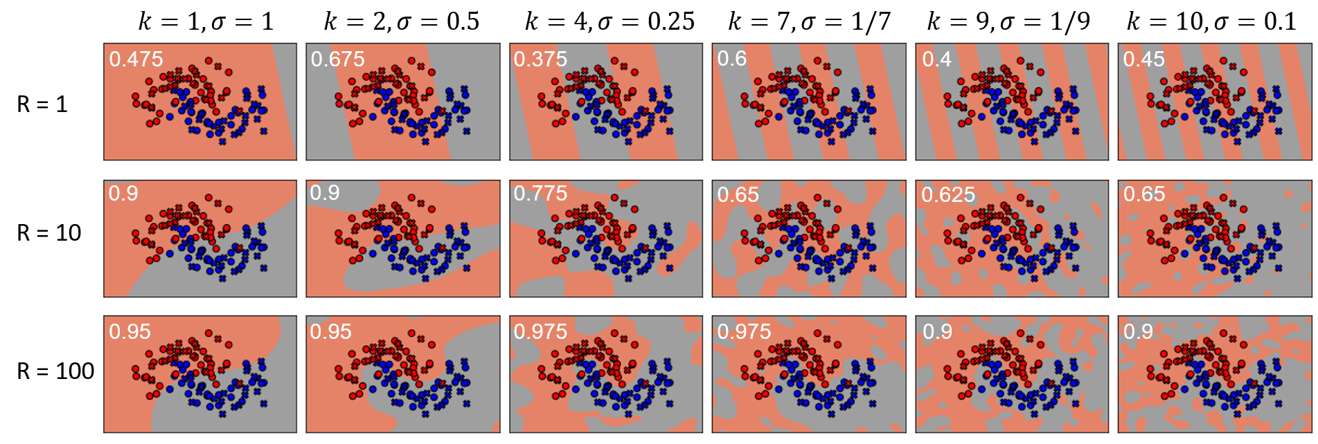
Fig. 6 illustrates the performance of moon dataset classifiers using circuits with 10 input photons and random Fourier features of different dimensions, i.e. and the same decision boundary as in Eq. (17). The circuit with input 10 photons can probe a range of kernel resolutions within one order of magnitude, e.g: for , the accessible resolutions are ; six of these are shown in Fig. 6 to illustrate the working principle of quantum-enhanced RKS. The decision boundary of smaller is considerably noisier than for larger . This is because the kernel with smaller resolution has a narrower peak, and hence, predictions far away from the training data points cannot be made. The random Fourier features with higher dimensionality provides a better approximation to the kernel, thus suppressing the noise around training data points while improving the classification accuracy. The optimal resolution for the moon dataset is and for .
III.4 Resource requirements for each scheme
Each of the classification methods has different strengths and limitations in terms of the resource requirements, i.e. number of distinct circuit evaluations for performing training and predictions, summarized in Tab. 1. Here, we are concerned only with number of distinct circuit evaluations required to perform training and prediction, since the quantum resources are much more precious than the classical resources in the NISQ era. For the variational circuit, the data features are directly encoded, but the beam splitters and phase shifters in the trainable circuit blocks need to be optimized in the training step. Hence, the training resource per optimization loop is , where , , and are the number of training data, the dimension of the data features, and the number of trainable circuit and observable parameters, respectively. More Fourier frequencies can be obtained with larger photon numbers but require larger for universality, increasing the training time. Prediction requires reconfiguration of the encoding phase shifters, which can however be performed in parallel.
| Schemes | Training time | Prediction time |
|---|---|---|
| Variational methods | D | |
| Kernel methods | N | |
| Random kitchen sinks | R |
Kernel methods, on the other hand, encode the differences between data inputs using one phase shifter and the training is outsourced to a classical computer, therefore the resources for training scale only with the number of training data, i.e. . The Gaussian kernel with different resolutions can be accessed with a fixed circuit by considering different observables; Gaussian kernels with higher resolutions are better approximated for circuits with larger numbers of input photons. In contrast to the variational methods, different phase shifter settings are required to make predictions on new data. Random kitchen sinks have similar advantages to kernel methods, i.e. fixed circuit and different resolutions can be accessed by different observables, but have a better scaling with number of input data points, where is the number of random features chosen. The predictions require circuit settings regardless of the dimension of the data features.
IV Conclusion
The data-embedding process is a bottleneck which must be addressed Harrow 2020 in order to fully leverage the potential of quantum machine learning algorithms. In this paper, we addressed the data encoding problem by proposing a more gate-efficient bosonic encoding method. Our method has three potential advantages. First, it allows for a more efficient data encoding by modulating all Fock basis simultaneously using only one phase shifter, regardless of the input photon number. Second, the circuits employed a kernel-like trick, where nonlinearity is outsourced to quantum feature maps, i.e. the data-encoding phase shifter that encode the classical data into the high-dimensional Fock space Havlíček et al. 2019; Schuld and Killoran 2019, avoiding the need of the experimental hard-to-implement nonlinear optical components. Subsequently, the expressive power of the circuit can be controlled by the number of input photons, while requiring fewer encoding layers compared to the qubit-based architecture Schuld et al. 2021; Pérez-Salinas et al. 2020. Finally, the circuits can be trained to implement commonly-used kernels with well-understood properties such as the Gaussian kernel.
Even though our photonic models are inspired by the BosonSampling circuits Aaronson and Arkhipov 2011, we do not expect the arguments about the BosonSampling’s classical non-simulability to hold for our circuits, for three reasons: (1) The model output is expectation values, not samples. (2) Our phoronic circuits are not sampled from the Haar random distribution. (3) The assumption of is relaxed, where is the number of optical modes and is the number of input photons. Even so, there exist other benefits of studying the use of this class of circuit as quantum machine learning models. Quantum machine learning is still in its infancy, and it is still unclear how to rigorously define a quantum advantage for generic machine learning problems Schuld and Killoran 2022. In this work, we focused on a specific problem in this field, the data-encoding problem, showing using simple quantum machine learning models how bosonic circuits may enable more efficient data uploading. We expect our conclusions to be valid for other classes of quantum machine learning models which may be hard to classically simulate. In addition, we believe our photonic models will serve as primitive quantum machine learning model Schuld and Killoran 2022 that inspire researchers in the field to develop other photonic quantum machine learning algorithms that possess quantum advantages. Recently, the awareness of the importance of the energy aspect of quantum algorithms has been raised Auffeves 2021. Although the energy aspect of our quantum circuits is not studied, our models could inspire an application-oriented framework to compare the energy consumption of quantum machine learning based on different platforms.
While the dimension of the Fock space grows (exponentially) with photon number and spatial modes, improving the expressive power, this is accompanied by higher sensitivity to optical losses and the need for more detection events in order to accurately sample all of the required output observables. Moreover, there exists a trade-off between the model’s expressive power and ability to generalize, where circuits with higher expressive power can suffer from larger generalization errors, i.e. over-fitting Banchi et al. 2021; Caro et al. 2021b and trainability issue Holmes et al. 2022. One potential way to mitigates these issues is to define the quantum machine learning models in projected Fock spaces, which may lead to potential quantum advantages Huang et al. 2021.
We proposed three different ways with different resource requirements to perform binary classification using linear quantum photonics circuits (QPCs). (1) Variational quantum classifiers that classify data points directly on the high-dimensional Fock space, while (2) and (3) implement Gaussian kernel for classical kernel machines directly or using the random kitchen sinks algorithm, sampling kernels with different resolutions in parallel. The random kitchen sink approach could be further improved by sampling the random features from a data-optimized distribution using fault-tolerant quantum computers Yamasaki et al. 2020; Yamasaki and Sonoda 2021. A linear QPC with three spatial modes and up to 10 input photons equipped with photon-number resolving detectors is sufficient to show a proof of concept experiment for all of the proposed approaches. Therefore, our proposed architecture can be implemented with current technology, such as integrated photonic circuits Carolan et al. 2015; Zhong et al. 2018; Hoch et al. 2021 or bulk optics Wang et al. 2019 used for BosonSampling experiments Brod et al. 2019. Other experimental aspects such as the impact of the degree of multi-photon distinguishability and exponentially-scaling photon losses on expressive power are subject for future research.
While this article investigated the expressive power of the linear QPCs, the trainability and generalization power of the linear QPCs remains an open question. Apart from the gradient-free method used in this article for QML model training, gradient-based methods with analytical gradient Schuld et al. 2019; Banchi and Crooks 2021; Wierichs et al. 2022 can potentially boost the training speed. However, current analytical gradient evaluation methods only apply to the photonic circuit with 1-photon input Fock state Kerenidis et al. 2021 or continuous variable quantum photonic systems Banchi et al. 2020; Miatto and Quesada 2020; Yao and Miatto 2021; Yao et al. 2022. Hence, more research needs to be done to find the analytical gradient for the quantum photonic circuits with general input Fock state, which requires the differentiation of the permanents of the transfer matrix. It will also be interesting to see the effect of different input states, i.e. coherent states and squeezed states on the expressive power, trainability, and generalization power of the linear QPCs Afek et al. 2010. It will be interesting to further explore the translation of ideas between classical and quantum photonic circuits for machine learning.
Acknowledgements.
This research was supported by the National Research Foundation, Prime Minister’s Office, Singapore, the Ministry of Education, Singapore under the Research Centres of Excellence programme, and the Polisimulator project co-financed by Greece and the EU Regional Development Fund.
Appendix A General encoding scheme for 1D frequency spectrum
In Sec.II.2.1, we have derived the frequency spectrum for linear QPCs with single data encoding block that consists only one data encoding phase shifter. In this section, we broaden the frequency spectrum by adding more data encoding phase shifters into the same layer (series encoding) and different layers (parallel encoding). In the series encoding scheme [Fig.7(a)], we consider linear QPCs with single data encoding block that consists of phase shifters, i.e. the highest possible number of phase shifters that can be placed within a data encoding block. For parallel encoding scheme [Fig.7(b)], the phase shifters are equally distributed among data encoding blocks. One could consider different combinations of phase shifters in each layers and the expressive power will change accordingly.
As shown in Sec.II.2.1, the size of the frequency spectrum of a mode linear QPC with one data encoding phase shifter is given by , where (two additional subscripts are added for clarity) denotes the size of frequency spectrum realizable by linear QPCs with input photons and data encoding blocks, each block consists of data encoding phase shifters. For series encoding (), we can place one data encoding phase shifter per mode on the first mode, each encodes phase proportional to its mode number [Fig.7(a)], i.e. phase shift with denotes the mode number. The range of phases that could pick-up by photon is , where the lower (upper) bound is obtained when all photon passes through the last (second last) mode. Hence, the size of the frequency spectrum is . Identical range of phases is also apply to the parallel encoding scheme, where the lower (upper) bound is achieved when none (all) of the photon passes through the first mode on each layer, thus, .
Appendix B Encoding scheme to generate full frequency spectrum for multi-dimensional Fourier series
In this section, we will introduce the series and parallel encoding schemes that can generate a full frequency spectrum for multi-dimensional Fourier series. For series encoding scheme [Fig.7(c)], one would need phase shifters to encode the positive phases of -dimensional degree 1 Fourier series, i.e. . For example, one can use 7 phase shifters to encode . Then, the frequency spectrum of dimensional degree Fourier series, i.e. with and can be generated using input photons. On the other hand, the same set of frequency spectrum can be generated using data encoding blocks, each consists of one data encoding phase shifter that encodes one data feature. [Fig.7(d)].
References
- De Marinis et al. (2019) L. De Marinis, M. Cococcioni, P. Castoldi, and N. Andriolli, Photonic neural networks: A survey, IEEE Access 7, 175827 (2019).
- Hamerly et al. (2019) R. Hamerly, L. Bernstein, A. Sludds, M. Soljačić, and D. Englund, Large-scale optical neural networks based on photoelectric multiplication, Phys. Rev. X 9, 021032 (2019).
- Roques-Carmes et al. (2020) C. Roques-Carmes, Y. Shen, C. Zanoci, M. Prabhu, F. Atieh, L. Jing, T. Dubček, C. Mao, M. R. Johnson, V. Čeperić, et al., Heuristic recurrent algorithms for photonic Ising machines, Nat. Commun. 11, 249 (2020).
- Shastri et al. (2021) B. J. Shastri, A. N. Tait, T. F. de Lima, W. H. Pernice, H. Bhaskaran, C. D. Wright, and P. R. Prucnal, Photonics for artificial intelligence and neuromorphic computing, Nat. Photonics 15, 102 (2021).
- Peruzzo et al. (2014) A. Peruzzo, J. McClean, P. Shadbolt, M.-H. Yung, X.-Q. Zhou, P. J. Love, A. Aspuru-Guzik, and J. L. O’Brien, A variational eigenvalue solver on a photonic quantum processor, Nat. Commun. 5, 4213 (2014).
- Mitarai et al. (2018) K. Mitarai, M. Negoro, M. Kitagawa, and K. Fujii, Quantum circuit learning, Phys. Rev. A 98, 032309 (2018).
- Benedetti et al. (2019) M. Benedetti, E. Lloyd, S. Sack, and M. Fiorentini, Parameterized quantum circuits as machine learning models, Quantum Sci. Technol. 4, 043001 (2019).
- Schuld et al. (2020) M. Schuld, A. Bocharov, K. M. Svore, and N. Wiebe, Circuit-centric quantum classifiers, Phys. Rev. A 101, 032308 (2020).
- Fujii and Nakajima (2021) K. Fujii and K. Nakajima, Quantum Reservoir Computing: A Reservoir Approach Toward Quantum Machine Learning on Near-Term Quantum Devices (Springer, Singapore, 2021) pp. 423–450.
- Goto et al. (2021) T. Goto, Q. H. Tran, and K. Nakajima, Universal approximation property of quantum machine learning models in quantum-enhanced feature spaces, Phys. Rev. Lett. 127, 090506 (2021).
- Lloyd et al. (2020) S. Lloyd, M. Schuld, A. Ijaz, J. Izaac, and N. Killoran, Quantum embeddings for machine learning, arXiv:2001.03622 [quant-ph] 10.48550/arXiv.2001.03622 (2020).
- Chatterjee and Yu (2016) R. Chatterjee and T. Yu, Generalized coherent states, reproducing kernels, and quantum support vector machines, arXiv:1612.03713 [quant-ph] 10.48550/arXiv.1612.03713 (2016).
- Schuld and Killoran (2019) M. Schuld and N. Killoran, Quantum machine learning in feature Hilbert spaces, Phys. Rev. Lett. 122, 040504 (2019).
- Steinbrecher et al. (2019) G. R. Steinbrecher, J. P. Olson, D. Englund, and J. Carolan, Quantum optical neural networks, npj Quantum Inf. 5, 60 (2019).
- Killoran et al. (2019) N. Killoran, T. R. Bromley, J. M. Arrazola, M. Schuld, N. Quesada, and S. Lloyd, Continuous-variable quantum neural networks, Phys. Rev. Research 1, 033063 (2019).
- Bartkiewicz et al. (2020) K. Bartkiewicz, C. Gneiting, A. Černoch, K. Jiráková, K. Lemr, and F. Nori, Experimental kernel-based quantum machine learning in finite feature space, Sci Rep 10, 12356 (2020).
- Taballione et al. (2021) C. Taballione, R. van der Meer, H. J. Snijders, P. Hooijschuur, J. P. Epping, M. de Goede, B. Kassenberg, P. Venderbosch, C. Toebes, H. van den Vlekkert, et al., A universal fully reconfigurable 12-mode quantum photonic processor, Mater. Quantum. Technol 1, 035002 (2021).
- Chabaud et al. (2021) U. Chabaud, D. Markham, and A. Sohbi, Quantum machine learning with adaptive linear optics, Quantum 5, 496 (2021).
- Ghobadi (2021) R. Ghobadi, Nonclassical kernels in continuous-variable systems, Phys. Rev. A 104, 052403 (2021).
- Havlíček et al. (2019) V. Havlíček, A. D. Córcoles, K. Temme, A. W. Harrow, A. Kandala, J. M. Chow, and J. M. Gambetta, Supervised learning with quantum-enhanced feature spaces, Nature 567, 209 (2019).
- Schuld and Petruccione (2021) M. Schuld and F. Petruccione, Machine Learning with Quantum Computers (Springer, Switzerland, 2021).
- Schuld (2021) M. Schuld, Supervised quantum machine learning models are kernel methods, arXiv:2101.11020 [quant-ph] 10.48550/arXiv.2101.11020 (2021).
- Pérez-Salinas et al. (2020) A. Pérez-Salinas, A. Cervera-Lierta, E. Gil-Fuster, and J. I. Latorre, Data re-uploading for a universal quantum classifier, Quantum 4, 226 (2020).
- Schuld et al. (2021) M. Schuld, R. Sweke, and J. J. Meyer, Effect of data encoding on the expressive power of variational quantum-machine-learning models, Phys. Rev. A 103, 032430 (2021).
- Pérez-Salinas et al. (2021) A. Pérez-Salinas, D. López-Núñez, A. García-Sáez, P. Forn-Díaz, and J. I. Latorre, One qubit as a universal approximant, Phys. Rev. A 104, 012405 (2021).
- Li and Deng (2022) W. Li and D.-L. Deng, Recent advances for quantum classifiers, Sci. China: Phys. Mech. Astron. 65, 1 (2022).
- Dutta et al. (2021) T. Dutta, A. Pérez-Salinas, J. P. S. Cheng, J. I. Latorre, and M. Mukherjee, Realization of an ion trap quantum classifier, arXiv:2106.14059 [quant-ph 10.48550/arXiv.2106.14059 (2021).
- Kusumoto et al. (2021) T. Kusumoto, K. Mitarai, K. Fujii, M. Kitagawa, and M. Negoro, Experimental quantum kernel trick with nuclear spins in a solid, npj Quantum Inf 7, 1 (2021).
- Peters et al. (2021) E. Peters, J. Caldeira, A. Ho, S. Leichenauer, M. Mohseni, H. Neven, P. Spentzouris, D. Strain, and G. N. Perdue, Machine learning of high dimensional data on a noisy quantum processor, npj Quantum Inf. 7, 1 (2021).
- Ren et al. (2022) W. Ren, W. Li, S. Xu, K. Wang, W. Jiang, F. Jin, X. Zhu, J. Chen, Z. Song, P. Zhang, et al., Experimental quantum adversarial learning with programmable superconducting qubits, arXiv:2204.01738 [quant-ph] 10.48550/arXiv.2204.01738 (2022).
- Tangpanitanon et al. (2020) J. Tangpanitanon, S. Thanasilp, N. Dangniam, M.-A. Lemonde, and D. G. Angelakis, Expressibility and trainability of parametrized analog quantum systems for machine learning applications, Phys. Rev. Research 2, 043364 (2020).
- Abbas et al. (2021) A. Abbas, D. Sutter, C. Zoufal, A. Lucchi, A. Figalli, and S. Woerner, The power of quantum neural networks, Nat. Comput. Sci. 1, 403 (2021).
- Holmes et al. (2022) Z. Holmes, K. Sharma, M. Cerezo, and P. J. Coles, Connecting ansatz expressibility to gradient magnitudes and barren plateaus, PRX Quantum 3, 010313 (2022).
- Caro et al. (2021a) M. C. Caro, H.-Y. Huang, M. Cerezo, K. Sharma, A. Sornborger, L. Cincio, and P. J. Coles, Generalization in quantum machine learning from few training data, arXiv:2111.05292 [quant-ph] 10.48550/arXiv.2111.05292 (2021a).
- Giovannetti et al. (2008) V. Giovannetti, S. Lloyd, and L. Maccone, Quantum random access memory, Phys. Rev. Lett. 100, 160501 (2008).
- Harrow et al. (2009) A. W. Harrow, A. Hassidim, and S. Lloyd, Quantum algorithm for linear systems of equations, Phys. Rev. Lett. 103, 150502 (2009).
- Wiebe et al. (2012) N. Wiebe, D. Braun, and S. Lloyd, Quantum algorithm for data fitting, Phys. Rev. Lett. 109, 050505 (2012).
- Lloyd et al. (2013) S. Lloyd, M. Mohseni, and P. Rebentrost, Quantum algorithms for supervised and unsupervised machine learning, arXiv:1307.0411 [quant-ph] 10.48550/arXiv.1307.0411 (2013).
- Lloyd et al. (2014) S. Lloyd, M. Mohseni, and P. Rebentrost, Quantum principal component analysis, Nat. Phys. 10, 631 (2014).
- Rebentrost et al. (2014) P. Rebentrost, M. Mohseni, and S. Lloyd, Quantum support vector machine for big data classification, Phys. Rev. Lett. 113, 130503 (2014).
- Biamonte et al. (2017) J. Biamonte, P. Wittek, N. Pancotti, P. Rebentrost, N. Wiebe, and S. Lloyd, Quantum machine learning, Nature 549, 195 (2017).
- Dunjko and Briegel (2018) V. Dunjko and H. J. Briegel, Machine learning & artificial intelligence in the quantum domain: a review of recent progress, Rep. Prog. Phys. 81, 074001 (2018).
- Tang (2021) E. Tang, Quantum principal component analysis only achieves an exponential speedup because of its state preparation assumptions, Phys. Rev. Lett. 127, 060503 (2021).
- Cotler et al. (2021) J. Cotler, H.-Y. Huang, and J. R. McClean, Revisiting dequantization and quantum advantage in learning tasks, arXiv:2112.00811 [quant-ph] 10.48550/arXiv.2112.00811 (2021).
- Lloyd et al. (2016) S. Lloyd, S. Garnerone, and P. Zanardi, Quantum algorithms for topological and geometric analysis of data, Nat. Commun. 7, 1 (2016).
- Harrow (2020) A. W. Harrow, Small quantum computers and large classical data sets, arXiv:2004.00026 [quant-ph] 10.48550/arXiv.2004.00026 (2020).
- Liu et al. (2021) Y. Liu, S. Arunachalam, and K. Temme, A rigorous and robust quantum speed-up in supervised machine learning, Nat. Phys. 17, 1013 (2021).
- Carleson (1966) L. Carleson, On convergence and growth of partial sums of Fourier series, Acta Math. 116, 135 (1966).
- Weisz (2012) F. Weisz, Summability of multi-dimensional trigonometric fourier series, arXiv:1206.1789 [math.CA] 10.48550/arXiv.1206.1789 (2012).
- Scheel (2004) S. Scheel, Permanents in linear optical networks, quant-ph/0406127 10.48550/arXiv.quant-ph/0406127 (2004).
- Reck et al. (1994) M. Reck, A. Zeilinger, H. J. Bernstein, and P. Bertani, Experimental realization of any discrete unitary operator, Phys. Rev. Lett. 73, 58 (1994).
- Clements et al. (2016) W. R. Clements, P. C. Humphreys, B. J. Metcalf, W. S. Kolthammer, and I. A. Walmsley, Optimal design for universal multiport interferometers, Optica 3, 1460 (2016).
- Bell and Walmsley (2021) B. A. Bell and I. A. Walmsley, Further compactifying linear optical unitaries, APL Photonics 6, 070804 (2021).
- Motes et al. (2015) K. R. Motes, J. P. Olson, E. J. Rabeaux, J. P. Dowling, S. J. Olson, and P. P. Rohde, Linear optical quantum metrology with single photons: Exploiting spontaneously generated entanglement to beat the shot-noise limit, Phys. Rev. Lett. 114, 170802 (2015).
- Olson et al. (2017) J. P. Olson, K. R. Motes, P. M. Birchall, N. M. Studer, M. LaBorde, T. Moulder, P. P. Rohde, and J. P. Dowling, Linear optical quantum metrology with single photons: Experimental errors, resource counting, and quantum cramér-rao bounds, Phys. Rev. A 96, 013810 (2017).
- Johnson (2014) S. G. Johnson, The NLopt nonlinear-optimization package (2014).
- Powell (2009) M. J. Powell, The BOBYQA algorithm for bound constrained optimization without derivatives, Cambridge NA Report NA2009/06, University of Cambridge, Cambridge , 26 (2009).
- (58) The nonlinear optical elements enables the realization of two qubit entangling gates, while arbitrary single qubit rotations can be realized using linear optics such as beam splitter and phase shifters. By considering the dual-rail photonic qubit, our circuit could perform universal quantum computation, and the Fourier coefficients arguments follows from Ref.Schuld et al. 2021.
- Fox (2006) A. M. Fox, Quantum optics: an introduction, Vol. 15 (Oxford university press, 2006).
- Pedregosa et al. (2011) F. Pedregosa, G. Varoquaux, A. Gramfort, V. Michel, B. Thirion, O. Grisel, M. Blondel, P. Prettenhofer, R. Weiss, V. Dubourg, J. Vanderplas, A. Passos, D. Cournapeau, M. Brucher, M. Perrot, and E. Duchesnay, Scikit-learn: Machine learning in python, J. Mach. Learn. Res. 12, 2825–2830 (2011).
- McClean et al. (2018) J. R. McClean, S. Boixo, V. N. Smelyanskiy, R. Babbush, and H. Neven, Barren plateaus in quantum neural network training landscapes, Nat. Commun. 9, 4812 (2018).
- Wang et al. (2021a) S. Wang, E. Fontana, M. Cerezo, K. Sharma, A. Sone, L. Cincio, and P. J. Coles, Noise-induced barren plateaus in variational quantum algorithms, Nat. Commun. 12, 1 (2021a).
- Marrero et al. (2021) C. O. Marrero, M. Kieferová, and N. Wiebe, Entanglement-induced barren plateaus, PRX Quantum 2, 040316 (2021).
- Bittel and Kliesch (2021) L. Bittel and M. Kliesch, Training variational quantum algorithms is NP-hard – even for logarithmically many qubits and free fermionic systems, Phys. Rev. Lett. 127, 120502 (2021).
- Thanasilp et al. (2021) S. Thanasilp, S. Wang, N. A. Nghiem, P. J. Coles, and M. Cerezo, Subtleties in the trainability of quantum machine learning models, arXiv:2110.14753 [quant-ph] 10.48550/arXiv.2110.14753 (2021).
- Arrasmith et al. (2021) A. Arrasmith, M. Cerezo, P. Czarnik, L. Cincio, and P. J. Coles, Effect of barren plateaus on gradient-free optimization, Quantum 5, 558 (2021).
- Haug et al. (2021) T. Haug, C. N. Self, and M. Kim, Large-scale quantum machine learning, arXiv:2108.01039 [quant-ph] 10.48550/arXiv.2108.01039 (2021).
- Schölkopf and Smola (2002) B. Schölkopf and A. Smola, Learning with Kernels: Support Vector Machines, Regularization, Optimization, and Beyond, Adaptive Computation and Machine Learning (MIT Press, Cambridge, MA, USA, 2002) p. 644.
- Hofmann et al. (2008) T. Hofmann, B. Schölkopf, and A. J. Smola, Kernel methods in machine learning, Annals of Statistics 36, 1171 (2008).
- Mercer (1909) J. Mercer, Functions of positive and negative type and their connection with the theory of integral equations, Phil. Trans. R. Soc. Lond. A 209, 415 (1909).
- Schölkopf et al. (2001) B. Schölkopf, R. Herbrich, and A. J. Smola, A generalized representer theorem, in Computational Learning Theory, edited by D. Helmbold and B. Williamson (Springer Berlin Heidelberg, Berlin, Heidelberg, 2001) pp. 416–426.
- Bishop (2006) C. M. Bishop, Pattern Recognition and Machine Learning (Information Science and Statistics) (Springer-Verlag, Berlin, Heidelberg, 2006).
- Theodoridis (2015) S. Theodoridis, Machine Learning: A Bayesian and Optimization Perspective, 1st ed. (Academic Press, Inc., USA, 2015).
- Huang et al. (2021) H.-Y. Huang, M. Broughton, M. Mohseni, R. Babbush, S. Boixo, H. Neven, and J. R. McClean, Power of data in quantum machine learning, Nat. Commun. 12, 2631 (2021).
- Wang et al. (2021b) X. Wang, Y. Du, Y. Luo, and D. Tao, Towards understanding the power of quantum kernels in the NISQ era, Quantum 5, 531 (2021b).
- Micchelli et al. (2006) C. A. Micchelli, Y. Xu, and H. Zhang, Universal kernels, J. Mach. Learn. Res. 7, 2651–2667 (2006).
- Steinwart and Christmann (2008) I. Steinwart and A. Christmann, Support vector machines, 1st ed. (Springer Publishing Company, Incorporated, New York, 2008).
- Rahimi and Recht (2007) A. Rahimi and B. Recht, Random features for large-scale kernel machines, in Advances in Neural Information Processing Systems, Vol. 20, edited by J. Platt, D. Koller, Y. Singer, and S. Roweis (Curran Associates, Inc., Red Hook, NY, USA, 2007).
- Rahimi and Recht (2008a) A. Rahimi and B. Recht, Uniform approximation of functions with random bases, in 2008 46th Annual Allerton Conference on Communication, Control, and Computing (2008) pp. 555–561.
- Rahimi and Recht (2008b) A. Rahimi and B. Recht, Weighted sums of random kitchen sinks: Replacing minimization with randomization in learning, in Proceedings of the 21st International Conference on Neural Information Processing Systems, NIPS’08 (Curran Associates Inc., Red Hook, NY, USA, 2008) p. 1313–1320.
- Wilson et al. (2018) C. Wilson, J. Otterbach, N. Tezak, R. Smith, A. Polloreno, P. J. Karalekas, S. Heidel, M. S. Alam, G. Crooks, and M. da Silva, Quantum kitchen sinks: An algorithm for machine learning on near-term quantum computers, arXiv:1806.08321 [quant-ph] 10.48550/arXiv.1806.08321 (2018).
- Noori et al. (2020) M. Noori, S. S. Vedaie, I. Singh, D. Crawford, J. S. Oberoi, B. C. Sanders, and E. Zahedinejad, Analog-quantum feature mapping for machine-learning applications, Phys. Rev. Applied 14, 034034 (2020).
- Hoerl and Kennard (1970) A. E. Hoerl and R. W. Kennard, Ridge regression: Biased estimation for nonorthogonal problems, Technometrics 12, 55 (1970).
- Aaronson and Arkhipov (2011) S. Aaronson and A. Arkhipov, The computational complexity of linear optics, in Proceedings of the forty-third annual ACM symposium on Theory of computing (2011) pp. 333–342.
- Schuld and Killoran (2022) M. Schuld and N. Killoran, Is quantum advantage the right goal for quantum machine learning?, arXiv:2203.01340 [quant-ph] 10.48550/arXiv.2203.01340 (2022).
- Auffeves (2021) A. Auffeves, Quantum technologies need a quantum energy initiative, arXiv:2111.09241 [quant-ph] 10.48550/arXiv.2111.09241 (2021).
- Banchi et al. (2021) L. Banchi, J. Pereira, and S. Pirandola, Generalization in quantum machine learning: a quantum information perspective, PRX Quantum 2, 040321 (2021).
- Caro et al. (2021b) M. C. Caro, E. Gil-Fuster, J. J. Meyer, J. Eisert, and R. Sweke, Encoding-dependent generalization bounds for parametrized quantum circuits, Quantum 5, 582 (2021b).
- Yamasaki et al. (2020) H. Yamasaki, S. Subramanian, S. Sonoda, and M. Koashi, Learning with optimized random features: Exponential speedup by quantum machine learning without sparsity and low-rank assumptions, in Advances in Neural Information Processing Systems, Vol. 33 (Curran Associates, Inc., Red Hook, NY, USA, 2020) pp. 13674–13687.
- Yamasaki and Sonoda (2021) H. Yamasaki and S. Sonoda, Exponential error convergence in data classification with optimized random features: Acceleration by quantum machine learning, arXiv:2106.09028 [quant-ph] 10.48550/arXiv.2106.09028 (2021).
- Carolan et al. (2015) J. Carolan, C. Harrold, C. Sparrow, E. Martín-López, N. J. Russell, J. W. Silverstone, P. J. Shadbolt, N. Matsuda, M. Oguma, M. Itoh, et al., Universal linear optics, Science 349, 711 (2015).
- Zhong et al. (2018) H.-S. Zhong, Y. Li, W. Li, L.-C. Peng, Z.-E. Su, Y. Hu, Y.-M. He, X. Ding, W. Zhang, H. Li, L. Zhang, Z. Wang, L. You, X.-L. Wang, X. Jiang, L. Li, Y.-A. Chen, N.-L. Liu, C.-Y. Lu, and J.-W. Pan, 12-photon entanglement and scalable scattershot boson sampling with optimal entangled-photon pairs from parametric down-conversion, Phys. Rev. Lett. 121, 250505 (2018).
- Hoch et al. (2021) F. Hoch, S. Piacentini, T. Giordani, Z.-N. Tian, M. Iuliano, C. Esposito, A. Camillini, G. Carvacho, F. Ceccarelli, N. Spagnolo, et al., Boson sampling in a reconfigurable continuously-coupled 3d photonic circuit, arXiv:2106.08260 [quant-ph] 10.48550/arXiv.2106.08260 (2021).
- Wang et al. (2019) H. Wang, J. Qin, X. Ding, M.-C. Chen, S. Chen, X. You, Y.-M. He, X. Jiang, L. You, Z. Wang, C. Schneider, J. J. Renema, S. Höfling, C.-Y. Lu, and J.-W. Pan, Boson sampling with 20 input photons and a 60-mode interferometer in a -dimensional Hilbert space, Phys. Rev. Lett. 123, 250503 (2019).
- Brod et al. (2019) D. J. Brod, E. F. Galvão, A. Crespi, R. Osellame, N. Spagnolo, and F. Sciarrino, Photonic implementation of boson sampling: a review, Adv. Photon. 1, 034001 (2019).
- Schuld et al. (2019) M. Schuld, V. Bergholm, C. Gogolin, J. Izaac, and N. Killoran, Evaluating analytic gradients on quantum hardware, Physical Review A 99, 032331 (2019).
- Banchi and Crooks (2021) L. Banchi and G. E. Crooks, Measuring analytic gradients of general quantum evolution with the stochastic parameter shift rule, Quantum 5, 386 (2021).
- Wierichs et al. (2022) D. Wierichs, J. Izaac, C. Wang, and C. Y.-Y. Lin, General parameter-shift rules for quantum gradients, Quantum 6, 677 (2022).
- Kerenidis et al. (2021) I. Kerenidis, J. Landman, and N. Mathur, Classical and quantum algorithms for orthogonal neural networks, arXiv:2106.07198 [quant-ph] 10.48550/arXiv.2106.07198 (2021).
- Banchi et al. (2020) L. Banchi, N. Quesada, and J. M. Arrazola, Training gaussian boson sampling distributions, Phys. Rev. A 102, 012417 (2020).
- Miatto and Quesada (2020) F. M. Miatto and N. Quesada, Fast optimization of parametrized quantum optical circuits, Quantum 4, 366 (2020).
- Yao and Miatto (2021) Y. Yao and F. M. Miatto, Fast differentiable evolution of quantum states under gaussian transformations, arXiv:2102.05742 [quant-ph] 10.48550/arXiv.2102.05742 (2021).
- Yao et al. (2022) Y. Yao, P. Cussenot, R. A. Wolf, and F. Miatto, Complex natural gradient optimization for optical quantum circuit design, Phys. Rev. A 105, 052402 (2022).
- Afek et al. (2010) I. Afek, O. Ambar, and Y. Silberberg, High-NOON states by mixing quantum and classical light, Science 328, 879 (2010).