The Impact of Three-phase Impedances on the Stability of DER systems
Abstract
In this work we explore impedance-based interactions that arise when inverter-connected distributed energy resources (DERs) inject real and reactive power to regulate voltage and power flows on three-phase unbalanced distribution grids. We consider two inverter control frameworks that compute power setpoints: a mix of volt/var and volt/watt control, and phasor-based control. On a two-bus network we isolate how line length, R/X ratio, and mutual impedances each affects the stability of the DER system. We validate our analysis through simulation of the two-bus network, and validate that the effects found extend to the IEEE 123-node feeder. Furthermore, we find that the impedance properties make it more challenging to design a stable DER system for certain placements of DER on this feeder.
Index Terms:
Distributed Energy Resources, eigenvalue analysis, impedances, inverter control, voltage regulationI Introduction
The last decade has seen rapid deployment of Distributed Energy Resources (DERs), though with simplistic controls compared to what is possible with the latest technology and policies. For example, the recent FERC Order 2222 requires regional operators to allow aggregated DERs to participate in transmission-level markets [1]. The actions of simplistically controlled DERs and those that provide transmission-level services can introduce great variability in power flows and voltages on distribution grids. If not addressed, this can challenge power quality and reliability, for example by causing voltage flicker, increasing voltage regulator taps, desensitizing relays, or even overloading substation transformers [2].
One standard solution to addressing power quality issues with DERs is through volt-var control. In addition, the IEEE 1547 standard [3] now requires DERs in high-penetration areas to have volt-watt capabilities. The concern is that simulations of local droop volt-var control inverters have indicated risks of oscillations [4]. Therefore it is important to assess whether and under what conditions DERs that operate under volt-var with volt-watt control may cause oscillations, and whether alternatives to droop control might better regulate voltages.
One growing class of alternatives to droop volt-var is incremental volt-var [5, 6]. The concept involves accumulating the inverter power setpoint to either minimize a local objective function [5], track a voltage reference [7, 8, 9], or track a voltage phasor [10]. These approaches remove steady state error, thereby keeping voltages within the 5% ANSI range. Furthermore they drive the system to an optimal state, which allows for optimal (economic) operation of the DERs while satisfying distribution-level constraints. Phasor-Based Control (PBC), which is based on the tracking of voltage phasors [10], has been implemented with incremental volt-var control [11]. In this work we will analyze DER systems operating under droop volt-var with volt-watt control, and PBC.
The state space model of PBC indicates that eigenvalue stability, which results in convergence as proven in [11], is dependent on the controller gains, the DER locations, and the network line impedances. In [11] we explored the impact of DER locations on the DER system’s stability. In this work we explore the impact of impedance properties. Three distinct metrics can characterize the impedance properties of a given network: line length, ratio, and mutual impedances. Through our analysis we make several remarks about the individual impact of these metrics, allowing one to predict the stability characteristics of a DER system prior to setting up a detailed simulation.
Some works have examined the stability of volt-var and volt-watt control as impedance information is varied. However, [12] simulates a two-bus system when varying line resistance, which changes both line length and ratio, rather than isolating the effect of each. Moreover, coupling between phases due to mutual impedances has been relatively unexplored in the literature apart from [7], which motivates us to include 3-phase unbalanced grids.
It is noted that impedances of real grids may be outdated or inaccurate. However, there is rich literature on estimating impedance models using sensor measurements, including distribution PMU measurements [13]. Some works sidestep computing impedances explicitly and instead use power-voltage sensitivity information to design controllers [14]. Even though these works do not explicitly compute the impedances, because the designs implicitly account for them, it is important to investigate their role in the stability of DER systems.
II Problem Formulation
II-A State Space Models
We first define state space models for DER systems operating under droop volt-var with volt-watt control, and PBC.
II-A1 Power Flow Linearization
Consider the Distflow [15] branch equation for a single-phase radial network
| (1) |
which approximates the relationship between voltage magnitudes and power flow from node to node with complex impedance .
We linearize (1) about a nominal voltage of by dropping the square term. Next, let be the squared voltage magnitude, the net real power, the net reactive power at node , and define vectors , , , on a network with nodes. Here refers to the substation node which is constant at . As done in [6, 9], we define the time step to be sufficiently large for the dynamics from inverters, lines, and loads to settle to steady state before new power injections are updated. The algebraic relationship between nodal power injections and squared nodal voltages at all nodes for time steps and becomes
| (2a) | |||
| (2b) | |||
where the entries of matrices R and X at the row and column are given by
| (3a) | |||
| (3b) | |||
is the unique set of lines (or path) connecting node back to the substation node. To extend (2a) to a three-phase system we consider each phase as a separate node and triple the set of nodes as done in [6, Appendix]. Each vector element in (2a) is replaced with a 3x1 vector, and each element of matrices R and X is replaced with a 3x3 block matrix. This gives and . The update equation for net nodal powers at time step is
| (4a) | |||
| (4b) | |||
II-A2 Droop Volt-Var with Volt-Watt State Space Model
The droop controlled inverter update is
| (5a) | |||
| (5b) | |||
where contain the droop curve slope parameters, and 1 is the nominal voltage of 1pu at all nodes. We have omitted the deadband and saturation portions of the standard curve, and instead analyze DER systems that operate on the sloped portion. Substituting the the power update equations (4a) and (4b) into equation (2b), we have
| (6) |
We subtract from both sides, noting that for these control laws , then substitute control laws (5) into (6), giving
| (7) |
Let our states be the voltage magnitude tracking error . We refer to the droop closed-loop system model as
| (8) |
where are changes in voltage magnitude from uncontrollable sources.
II-A3 PBC State Space Model
The PBC model has states defined as the voltage magnitude tracking errors and voltage phase angle tracking errors at all nodes. The voltage magnitude and phase angle references tend to be near and respectively. The inputs are the change in inverter power setpoints , at all nodes (see our previous work [11] for the moderl derivation). The PBC closed-loop system model is
| (9) |
where , and , which are the changes in voltage magnitude references and changes in voltage magnitude from uncontrollable sources, respectively. Likewise, , and .
For both models, the algebraic DistFlow equations and the proposed control laws form a closed-loop quasi-steady state dynamical system. The closed-loop dynamics matrix depends on the controller gain matrix and the impedance matrix . In previous work [11] we designed such that the eigenvalues of are stable, because a stable PBC system results in asymptotic phasor tracking and optimal DER operation. Here, we aim to understand how the impedance properties of affect the eigenvalues of .
II-B Impedance Metrics
The impedances in can be characterized by three metrics applied to the complex impedance block for each three-phase line. The first is ratio, which is defined as
| (10) |
The ratio is important for controlling DER systems because high ratio causes cross interactions between real power and reactive power and voltage magnitude and phase angle [16].
The next metric is phase ratios, which we define as
| (11a) | |||
| (11b) | |||
| (11c) | |||
The phase ratio is important for controlling DER systems because high mutual impedances () causes cross interaction between phases. For example, high mutual impedances cause power injections on phase A to also affect voltages on phase B and C.
The last metric is line length. The magnitude of
| (12) |
commonly represents the length of each balanced physical conductor line in a single-line system
A line length metric is less obvious for three-phase unbalanced systems where is a 3x3 matrix instead of a scalar. With as the largest singular value of , we will use
| (13) |
II-C Two-Bus Network
For the following three scenarios we use the two-bus circuit in Fig. 1. We analyze how varying each impedance metric changes the dominant (maximum magnitude) eigenvalue of the closed-loop system . We define the range of stabilizing controller gains as , where is the controller gain that puts the system’s dominant eigenvalue on the verge of instability. indicates the ease of designing a stabilizing controller, and the dominant eigenvalue predominantly determines the system trajectory.

II-C1 Line Length vs. Stabilizing Controller Gains
Consider the two-bus PBC example in Fig. 1 as a single phase system with scalar line impedance , which could represent the effective impedance of a complex circuit. Note that the line length is equal to the reactance . For PBC, and
| (14a) | |||
| (14b) | |||
For the droop control model, we have , , . Thus .
Proposition 1.
For PBC and droop control models applied to the Fig. 1 system, increasing line length reduces
Proof: For the PBC case, the eigenvalues of are . By setting , we solve for . As , . For the droop control case, , resulting in . As , .
II-C2 R/X Ratio vs. Stabilizing Controller Gains
Next we isolate the effect of ratio (10) on the stability of the DER system. We set , , , and . This makes .
The PBC matrix is
| (15) |
For the PBC matrix, we set and .
For droop control, the matrix is the upper half of the PBC , and .
Proposition 2.
For PBC and droop control models applied to the Fig. 1 system, increasing the line ratio (up to ) reduces .
Proof: Substituting (10) into (12) and rearranging gives , and from (10), . This allows us to express in terms of and . For the two-bus PBC system, the eigenvalues are
| (16) |
By setting ,
| (17) |
As , .
For the two-bus droop system, eigenvalues are
| (18) |
with critical gain of
| (19) |
For , increases decreases. For as , , but is less common on real grids.
To visualize the proposition, in Fig. 2 and Fig. 3 we set , and for six R/X ratios we vary and plot the dominant eigenvalue for PBC and droop control, respectively.


II-C3 Phase Ratio vs. Stabilizing Controller Gains
Next we isolate the effect of phase ratio (11) on the stability of the DER system. We set , , and . This makes . The PBC matrix is
| (20) |
and the droop control matrix is the upper half of .


The matrix for PBC and droop models are the same as the II-C2 section. For PBC, the eigenvalues are
| (21) | |||
| (22) |
and for droop control they are
| (23) | |||
| (24) |
The three-phase line length metric (13) prevents us from analytically solving for in terms of . Instead, we choose six pairs of (,) with different phase ratio such that for all pairs. We vary and plot the dominant eigenvalue for the PBC system in Fig. 4 and for the droop system in Fig. 5. We observe that
Remark 1.
- a)
For PBC, higher phase ratios results in longer closed-loop trajectory settling time,
- b)
For PBC, very high phase ratios can result in no stabilizing controller gains,
- c)
For droop control, varying phase ratios have no effect on stabilizing controller gains or trajectory settling time
The first bullet and was validated by simulating the two-bus example for in OpenDSS, where nonlinear power flow is solved between each power setpoint update. The simulation was omitted due to space constraints. The second bullet can be seen from the phase ratio case in Fig 4, and the third bullet is observed from Fig. 5.
III Results
III-A Two-Bus Simulations
First we validate the PBC stabilizing control gain range for from Fig. 2 by simulating the single-phase two-bus network in Fig. 6. The PQ bus load is , initial conditions are , and phasor reference are . The critical gain from the nonlinear simulation matches the one found by the linear analysis (). For this gain, we observe that unstable oscillations arise immediately.

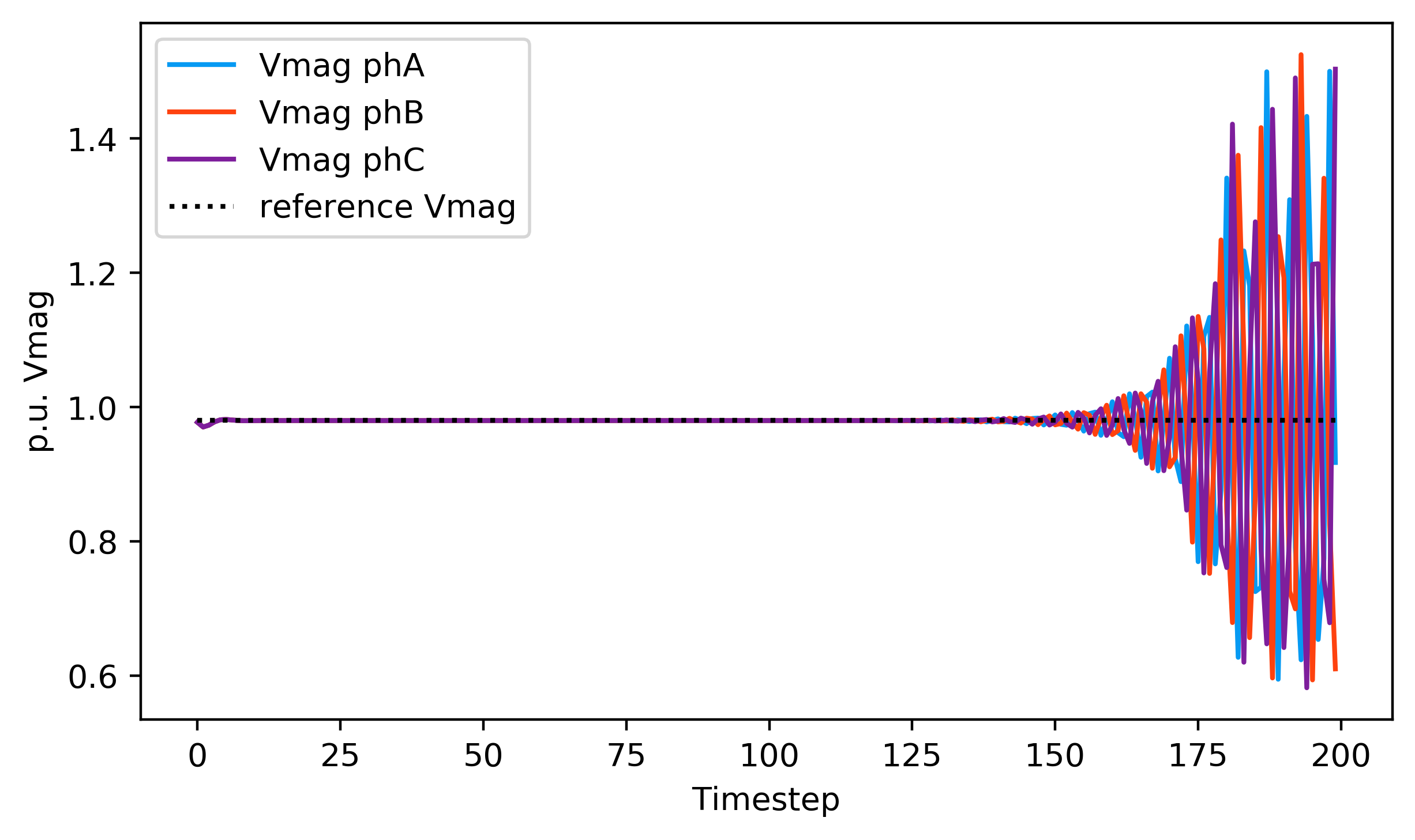
Next we validate the PBC stabilizing control gain range for from Fig. 4 by simulating the three-phase two-bus network in Fig. 7. The PQ bus load, initial conditions, and phasor references are the same as the previous paragraph, though applied to three phases. The critical gains from the nonlinear simulation matches the one found by the linear analysis (). For this gain, unstable oscillations begin after 150 seconds. This delay is concerning, indicating that oscillations from high phase ratio lines may be more difficult to detect than oscillations from high R/X ratio lines.
III-B Experiment Setup on Larger Feeders
III-B1 Disturbance Rejection Requirement for Droop Control
While stability of the droop model (8) ensures that no or in the worst case damped voltage oscillations occur, stability is not sufficient to guarantee the voltage magnitudes are driven inside the 5% ANSI range. This is because droop control admits a steady state error, which may land outside the 5% range depending on the system’s operating point.
One could evaluate a set of droop control parameters by how much the steady state error changes after a voltage step change disturbance . [17] derives the change in steady state error to be , with and defined in (8). We see that when , any disturbance will shift the steady state error by just as much (). Nonzero control gains contracts the steady state error, thereby providing some disturbance rejection capability.
III-B2 About the Heatmap Tool
In our previous work [11], we incorporated the PBC model (9) into a heatmap tool that visually illustrates good locations for configurations of DERs (actuator nodes) and associated sensors (performance nodes). The tool’s code can be downloaded at:
https://github.com/jaimiosyncrasy/heatMap. In this work, we extended the tool to work for the droop model (8).
The locations of actuator-performance node pairs (APNPs) enforces certain structural requirements on per configuration. An APNP is co-located if a DER and its associated sensor are at the same node. Additionally, the matrix structure is simplified by realistic assumptions about the configurations: all droop 3x3 blocks in representing three-phase nodes are diagonal, and for PBC . See Assumptions 1 and 2 of [11] for details.
For a given configuration operating under droop control, if we can find at least one such that (1) the closed-loop system is stable in the sense of Lyapunov, and (2) the steady state error contracts by at least 7% when , our tool indicates that the configuration and associated is good. For a configuration operating under PBC to be good, only requirement (1) is needed.
III-C Validation of the Two-Bus Remarks on Larger Feeder
We now determine whether Proposition 2 and remark 1 found for the two-bus network extend to the unbalanced IEEE 123-node feeder (123NF) [18]. We use the heatmap tool to find an -node configuration under PBC or droop control that is good on the original 123NF. Once found we record the best associated , which is the found that corresponds having the smallest dominant eigenvalue magnitude. Then we apply this best to the same configuration on a modified 123NF, where every line has a higher R/X or phase ratio with the same line length (13). If the configuration on the higher-ratio 123NF is no longer good, that result supports the remarks. Then we do the reverse. That is, we find a good configuration on the modified 123NF and apply the best associated to the original 123NF, noting whether the system is no longer good. If no longer good, that result contradicts the remarks.
Each entry of Table I records the percentage of results that support, with respect to a total of ten results that support or contradict the remarks. The experiments involve the original 123NF versus the 123NF that is modified to have the R/X ratio or phase ratio of every line multiplied by 1.5x. The first two columns of Table I supports Proposition 2. The third column supports remark 1.b). The last column, where phase ratios equally often support and contradict in the experiment, supports remark 1.c).
| R/X ratio | phase ratio | |||
|---|---|---|---|---|
| m | PBC, orig 1.5x | droop, orig 1.5x | PBC, orig 1.5x | droop, orig 1.5x |
| 1 | 100% | inconc. | 100 | 50% |
| 5 | 100% | 100% | 100% | 60% |
| 10 | 100% | 100% | 100% | 60% |
| 15 | N/A | 100 | N/A% | 50% |
III-D Branch Comparison on 123NF
In order to conduct an experiment that compares feeder branches with differing R/X and phase ratios, we first describe one of the heatmap tool’s placement process.
III-D1 Co-located Placement Process (CPP)
The CPP illustrates good places to place the next co-located APNP to maintain stability of the DER system. It iterates through every empty node in the feeder, fixing each as a candidate co-located APNP. Then, we generate a heatmap on the network, where a node’s color indicates whether the configuration created by appending the candidate APNP to the existing set of APNPs is good. If the node is blue, several (at least 7% of) matrices sampled from the parameter space defined in [11] make the configuration good. If the node is yellow, only a few were found, and if red, no matrices were found.
III-D2 Branch Comparison Experiment

We define two configurations of co-located APNPs, [node_8, node_53, node_57, node_66] and [node_8, node_53, node_57, node_74]. Note that has an APNP on branch [node_62 node_66], which has the highest three-phase R/X ratios and phase ratios, as measured by each node’s path to the substation.
We place on the 123NF operating under PBC, then run the CPP to find good locations for the fifth APNP, which is illustrated by the tool’s heatmap in Fig. 8. We run the CPP for thee more variations: controlled with PBC, droop controlled with , and droop controlled with . We tabulate the number of blue, yellow, and red nodes across the four runs in Fig. 9. The greater percentage of red nodes for both droop and PBC models indicates that placing co-located DER-sensor pairs on high-ratio branches makes it difficult to place subsequent DERs.

IV Conclusion
In this work we investigated the impact of network impedances on the stability of DER systems operating under droop and PBC models. We proved that long lines and high R/X ratios reduce the range of stabilizing controller gains (Proposition 1 and 2). Then, for PBC we found that high phase ratios reduce closed-loop settling time and can result in no stabilizing gains. We validated our 2-bus system analysis with simulations, and verified that the effects extend to the 123NF. Finally, we demonstrated that placing co-located DER-sensor pairs on high R/X and phase-ratio branches of the 123NF makes it difficult to place subsequent DERs.
In future work we will extend the branch comparison experiment to other large feeders. We will also accompany the analysis with large-scale simulations to validate the stability results. Finally, we seek to theoretically prove the observed relationship between high ratio branches and the ease of finding stabilizing controller gains.
Acknowledgements
We thank Daniel Tutt and Keith Moffatt for their insightful discussions. This work was supported by the U.S. Dept. of Energy, Award DE-EE0008008.
References
- [1] “FERC Opens Wholesale Markets to Distributed Resources: Landmark Action Breaks Down Barriers to Emerging Technologies, Boosts Competition.” News Release: Sept 17, 2020, Available: www.ferc.gov/news-events/news/ferc-opens-wholesale-markets-distributed-resources-landmark-action-breaks-down, Accessed 29 May 2021.
- [2] R. Seguin, J. Woyak, D. Costyk, J. Hambrick, and B. Mather, “High-Penetration PV Integration Handbook for Distribution Engineers,” 2016. power quality handbook, Mather.
- [3] “IEEE standard for interconnection and interoperability of distributed energy resources with associated electric power systems interfaces,” IEEE Std 1547-2018 (Revision of IEEE Std 1547-2003), 2018.
- [4] S. Chakraborty, A. Hoke, and B. Lundstrom, “Evaluation of multiple inverter volt-VAR control interactions with realistic grid impedances,” in IEEE Power and Energy Society General Meeting, July 2015.
- [5] M. Farivar, X. Zho, and L. Chen, “Local voltage control in distribution systems: An incremental control algorithm,” in 2015 IEEE International Conference on Smart Grid Communications (SmartGridComm), pp. 732–737, Nov. 2015.
- [6] A. Eggli, S. Karagiannopoulos, S. Bolognani, and G. Hug, “Stability analysis and design of local control schemes in active distribution grids,” pp. 1–1, Sep. 2020.
- [7] B. A. Robbins, C. N. Hadjicostis, and A. D. Domínguez-García, “A Two-Stage Distributed Architecture for Voltage Control in Power Distribution Systems,” IEEE Transactions on Power Systems, vol. 28, pp. 1470–1482, May 2013.
- [8] N. Li, G. Qu, and M. Dahleh, “Real-time decentralized voltage control in distribution networks,” in 52nd Annual Allerton Conference on Communication, Control, and Computing, pp. 582–588, Sep. 2014.
- [9] R. E. Helou, D. Kalathil, and L. Xie, “Communication-free voltage regulation in distribution networks with deep PV penetration,” in Hawaii International Conference on System Sciences, Jan. 2020.
- [10] A. v. Meier, E. L. Ratnam, K. Brady, K. Moffat, and J. Swartz, “Phasor-Based Control for Scalable Integration of Variable Energy Resources,” Energies, vol. ”13”, p. ”190”, Jan. 2020.
- [11] J. Swartz, B. Wais, E. Ratnam, and A. von Meier, “Visual Tool for Assessing Stability of DER Configurations on Three-Phase Radial Networks,” preprint arXiv:2011.07232, accepted to IEEE Powertech 2021, Nov. 2020.
- [12] J. H. Braslavsky, J. K. Ward, and L. Collins, “A stability vulnerability in the interaction between volt-var and volt-watt response functions for smart inverters,” in 2015 IEEE Conference on Control Applications (CCA), pp. 733–738, 2015.
- [13] K. Moffat, M. Bariya, and A. Von Meier, “Unsupervised impedance and topology estimation of distribution networks—limitations and tools,” IEEE Transactions on Smart Grid, vol. 11, no. 1, pp. 846–856, 2019.
- [14] J. Zhang, Z. Chen, C. He, Z. Jiang, and L. Guan, “Data-Driven-Based Optimization for Power System Var-Voltage Sequential Control,” IEEE Transactions on Industrial Informatics, vol. 15, pp. 2136–2145, 2019.
- [15] M. E. Baran and F. F. Wu, “Network reconfiguration in distribution systems for loss reduction and load balancing,” vol. 4, pp. 1401–1407, Apr. 1989.
- [16] A. von Meier, E. Stewart, A. McEachern, M. Andersen, and L. Mehrmanesh, “Precision micro-synchrophasors for distribution systems: A summary of applications,” IEEE Transactions on Smart Grid, vol. 8, pp. 2926–2936, Nov. 2017.
- [17] A. Singhal, V. Ajjarapu, J. Fuller, and J. Hansen, “Real-time local volt/var control under external disturbances with high PV penetration,” IEEE Transactions on Smart Grid, vol. 10, pp. 3849–3859, Jul. 2019.
- [18] IEEE Distribution Test Feeders. Available: http://sites.ieee.org/pes-testfeeders/resources/, Accessed 7 Nov. 2020.