.tif
Graph neural networks for simulating crack coalescence and propagation in brittle materials
Abstract
High-fidelity fracture mechanics simulations of multiple microcracks interaction via physics-based models quickly become computationally expensive as the number of microcracks increases. This work develops a Graph Neural Network (GNN) based framework to simulate fracture and stress evolution in brittle materials due to multiple microcracks’ interaction. The GNN framework is trained on the dataset generated by XFEM-based fracture simulator. Our framework achieves high prediction accuracy on the test set (compared to an XFEM-based fracture simulator) by engineering a sequence of GNN-based predictions. The first prediction stage determines Mode-I and Mode-II stress intensity factors (which can be used to compute the stress evolution by LEFM), the second prediction stage determines which microcracks will propagate, and the final stage actually propagates crack-tip positions for the selected microcracks to the next time instant. The trained GNN framework is capable of simulating crack propagation, coalescence and corresponding stress distribution for a wide range of initial microcrack configurations (from 5 to 19 microcracks) without any additional modification. Lastly, the framework’s simulation time shows speed-ups 6x-25x faster compared to an XFEM-based simulator. These characteristics, make our GNN framework an attractive approach for simulating microcrack propagation and stress evolution in brittle materials with multiple initial microcracks.
Keywords:
Machine Learning Simulator; Microcracks Coalescence; Graph Neural Networks; Brittle Materials; Extended Finite Element Method1 Introduction
Modeling the initiation, propagation, and interaction of cracks in engineering materials is critical for evaluating their performance and durability across various applications. Since its conception, the field of computational fracture mechanics continues to play a significant role in predicting crack initiation, propagation, coalescence and ultimate material failure. High-fidelity modeling techniques such as extended finite element method (XFEM) Belytschko1999XFEM, Belytschko2000RockXFEM, li2018review, meshfree methods garg2018meshfree, scaled boundary finite element method (SBFEM) SONG1997329, WOLF2000191, SONG2000211, song2018review, cohesive zone modeling (CZM) Park2011CZM, schwalbe2012guidelines, yuan2018critical, MOORE201846, and phase-field modeling (PFM) francfort1998revisiting, ambati2015review, ambati2016phase have provided efficient, scalable and reliable means to predict crack behavior in materials. A comprehensive review and comparative study of these methods can be found in egger2019discrete, sedmak2018computational and references therein.
Despite their success, high-fidelity simulation techniques may require extensive computational resources depending on the type of material, number of cracks, loading configuration and initial crack orientation. For instance, modeling microcrack nucleation, propagation and coalescence at the microstructural scale can be very computationally expensive depending on the number of microcracks and microstructural details. Understanding material failure at macroscale from microstructure could require simulating prohibitively large number of microcracks. For instance, when transitioning from a 2D problem to a realistic 3D microcrack coalescence problem, a domain may take several CPU-days to solve HUNTER201987. A possible solution to circumvent the burden of dimensionality involves reduced-order modeling techniques lucia2004reduced, oliver2017reduced, HUNTER201987.
Machine learning (ML) methods offer a promising way to develop such reduced order models. In the past few years, ML techniques have increasingly found applications in solid mechanics problems. Recent works have used ML methods to predict stress hotspots for different crystal configurations, apply tensor decomposition of complex materials, model the behavior of nonlinear materials, and predict complex stress and strain fields in composites MANGAL2018122, MANGAL20191, Wang2021Tensor, 8967240, HE2021114034, Yangeabd7416. ML techniques have also been applied to fracture mechanics problems PANDOLFI2021114078, LIU2020105, HAGHIGHAT2021114012, ZHANG2020112725, SAHA2021113452, osti_1765066, including simulating 2D crack propagation problems such as predicting structural response due to crack growth, predicting displacement of notched plates, and simulating crack growth in graphene FENG2021113885, IM2021114030, Lew2021DeepLM. In one of the recent studies MOORE201846, HUNTER201987, authors first used the high-fidelity model Hybrid Optimization Software Suite (HOSS) Knight2020HOSS, Euser_2019 to gather a large dataset of microcrack coalescence tests. The dataset was then used to train a graph-theory-inspired artificial neural network for predicting connecting cracks, along with an estimated time to failure of the system. Another recent study of ML for fracture mechanics implemented a molecular dynamic (MD) simulation model to gather a training dataset, which was then used along a convolutional long-short term memory (ConvLSTM) network for simulating crack growth HSU2020197. In their approach, the authors demonstrated that by converting the training input to a binary image depicting crack locations as black pixels and the surrounding space as white pixels, the ConvLSTM network was able to predict the next time-step for the crack path as a binary image. Although these studies apply ML to fracture mechanics, predicting dynamic crack propagation and stress evolution simulations of higher-complexity problems with varying number of initial microcracks has not yet been studied.
In this work we apply the Graph Network-based Simulator (GNS) to simulate multi-crack dynamics. The GNS framework was introduced in 2020 to simulate particle dynamics of fluids and deformable materials when interacting with a rigid body sanchezgonzalez2020learning. The GNS approach integrates graph theory along with three ML multi-layer perceptron (MLP) networks. The framework was used to represent up to 20k water, sand, and viscous fluid particles as nodes, and their neighboring interactions of energy, momentum, and/or gravitational force as message-passing edges; conceptually similar to nodes and connecting edges in neural networks. The information from the message-passing latent space and previous time-steps was used to predict the accelerations and future position of particles, with similar accuracy to conventional numerical integrators used in high-fidelity models. This work was extended to develop a mesh-based graph neural network, called MeshGraphNet pfaff2021learning to simulate finite element simulations of plate bending, flow over an airfoil, flow over a cylinder, and flag dynamics with high accuracy compared to the conventional models. Recenly, the GNS approach was applied for simulating the homogenized responses of polycrystals VLASSIS2020113299. In their work, the authors first developed a graph network representation for polycrystals using vertices for each crystal within the structure, and edges connecting the crystals which shared a face. They then used the GNS approach to predict energy functionals, and simulate anisotropic responses of polycrystals in phase-field fracture.
In our work we leverage advancements in graph neural networks (GNNs) to develop a framework (Microcrack-GNN) capable of simulating microcrack propagation and coalescence in brittle materials with high accuracy. We considered higher-complexity problems involving multiple microcracks (5 to 19). The structure of the Microcrack-GNN framework shown in Figure 1 consists of four GNNs; each GNN is intended to model an underlying physics component of microcrack mechanics. In the XFEM approach, propagating crack-tips are determined by their resulting stress distributions ZHUANG201413; computed using the superposition of Mode-I and Mode-II effects. We capture this relationship using two GNNs, -GNN and -GNN, predicting Mode-I and Mode-II stress intensity factors respectively. The third GNN, Class-GNN, predicts propagating vs non-propagating microcracks, capturing the quasi-static nature of the problem. Using these predictions, the fourth GNN, CProp-GNN, predicts the future positions of the crack-tips. By integrating each of these GNNs as shown in Figure 1, we demonstrate that the framework not only predicts crack coalescence and crack paths with high accuracy, but also stress distributions throughout the domain. We present a new data-driven approach which may serve as a baseline for simulating higher-complexity fracture problems with fewer computational resources and time requirements.

The paper is organized as follows. In Section 2, we describe the XFEM-based model used for gathering training and validation datasets, the graph network representation, the generation of nearest-neighbours, and the spatial message-passing procedure used for each GNN. In Section 3, we present a description of the problem set-up including the training-set, validation-set, and test-set, along with the set-up process for varying number of microcracks. In Section 4 , we introduce the structure for the implemented Microcrack-GNN. This includes detailed descriptions for the -GNN, -GNN, Class-GNN, and CProp-GNN. In Section 5, we report the cross-validation results for various training parameters. In Section 6, we present the Microcrack-GNN’s ability to predict microcrack propagation and coalescence until failure and microcrack length growth for cases involving 5, 8, 10, 12, 15, and 19 initial microcracks, error analyses for the predicted crack length growth, error analyses for the predicted final crack paths, error analyses for the predicted effective stress intensity factors, and performance comparison with two additional baseline networks. Finally, in Section 6 we compare the required simulation times until failure of the Microcrack-GNN versus the XFEM-based model when increasing the number of initial microcracks (from 5 to 19).
2 Methods
2.1 XFEM-based model
We use the open source XFEM-based model presented in SUTULA2018205, SUTULA2018225, SUTULA2018257 for simulating various cases of fracture mechanics for brittle materials. This framework (written in MATLAB) is capable of modeling propagation of multiple cracks with arbitrary orientations in a 2D domain. Additionally, the XFEM framework is capable of applying various crack growth criteria defined by the user, such as the minimum total energy, the maximum hoop stress, and the symmetric localization criteria. To speed up computation, the authors account only for changes in the fracture topology to compute the timewise force vectors, stiffness matrices, and mesh-enrichment at each crack-tip. They then use the domain-form interaction integral approach GONZALEZALBUIXECH2013129, Zhu2012Improved to compute the 2D stress intensity factors, and , taking into account the residual strain or stress of each crack, and their surface pressure. We use this model to generate a dataset of 2D fracture simulations with multiple microcrack propagation and coalescence.
2.2 Graph Network Representation
In the GNN model, we describe the system as , where represents all crack-tips as vertices, and represents all the edges in the graph. The edges representation, , includes edges connecting each crack-tip (i.e., for any positive integer where corresponds to the total number of microcracks) to other crack-tips within a zone of influence (as shown in Figures 3(a) - 3(b)), as well as their edges to non-connecting crack-tips (i.e., outside the zone of influence).
The crack-tip vertices for a sequence of previous time-steps, , are defined by their timewise positions, , their nearest-neighboring crack-tips , as well as their initial orientation (i.e., , , or ).


| (1) |
Here and are the Cartesian coordinate positions and orientation (in radians) of vertex . Additionally, at every discretized time-step, the edges in the system will be defined by arrays, where is the index for the “sender” vertex, is the index for the “receiver” vertex (i.e., for any positive integer and , where corresponds to the total number of microcracks), and is a binary value specifying whether the “sender” vertex and the “receiver” vertex form part of the same pairwise neighbors. We note that when iterating through each crack-tip in the system, we set for . Using this representation, we define a series of neighbors for each microcrack in time sequence as
| (2) |
Here defines the current crack-tip (or “sender” node) at time , is the neighboring crack-tip (or “receiver” node) at time , and is a binary value informing the graph network whether and are within the same neighborhood at time .
2.3 Nearest-neighbor sets formulation
Next, we compute all microcrack tips that lie within a zone of influence of as depicted in Figure 3(c) and 3(d) by the white-dashed lines. Additionally, if a single crack-tip from a neighboring crack, , falls within the zone of influence of the current crack, (i.e., ) then the other crack-tip of the neighboring crack is also considered a neighboring vertex. In this case, a connecting edge is assigned as shown in Figure 3c by the red-dashed line. In a similar fashion, the neighbors of already-coalesced crack-tips are also shared with the neighbors of the connecting crack-tips, and vice-versa.
2.4 Spatial Message-Passing Process
The purpose of the spatial message-passing process in GNNs is to learn relationships of the latent space for the vertices, edges, and resulting nearest-neighbors dwivedi2020benchmark. In this work, the implemented message-passing process involves three main functions to update the system in time.
First, we develop the graph network representation for the vertices (crack-tips) and their feature vectors, as well as their respective nearest-neighbor configuration as described in Section 2.2 using equation (1). We then pass the resulting feature vector for the vertices as input to an encoder MLP, denoted as “v-MLP” in Figure 4, and represented by in equation (3a). The outputs from the vertices’ MLP encoder network, , are the encoded vertices’ embedding in the latent space for a sequence of time .
Second, we learn the relationship effects between vertex-edge-vertex interactions. We achieve this by applying an additional MLP encoder network to the resultant edges embedding obtained from equation (2). The edges MLP encoder network is denoted in Figure 4 with “e-MLP”, and depicted in equation (3b) as . As a result, the outputs from equation (3b), , are the encoded edges’ embedding describing the vertex-to-edge interactions in the latent space for the time sequence .
| (3) |

Lastly, we concatenate the encoders’ output for both the vertices’ embedding and for the vertex-edge-vertex embedding and pass it through the message-passing network. The message-passing MLP network, denoted by “G-MLP” in Figure 4, allows the network to learn information from the latent space between the crack-tips and edge features, and their interaction klicpera2020directional, li2017gated, zhang2020dynamic, gilmer2017neural. To perform the message-passing phase, a series of update steps are taken on the message-passing MLP. We note that depending on the complexity of the problem, the required number of update steps may vary. Following a similar approach as presented in Scarselli2009Graph, battaglia2018relational, battaglia2016interaction, we initially chose four update steps for all GNNs presented in this work. However, after cross validation (Section 5) the optimal number of message passing steps obtained was . As a result a one-hot encoded feature vector describing the latent space vertex-edge-vertex interactions, , is obtained as
| (4) |
Here is the message-passing MLP network, represents all nearest-neighbors of all microcracks, and describes all nearest-neighbors of microcrack (i.e., at ).
3 Simulations set-up
3.1 Training-set and Validation-set
As mentioned in Section 2.1, we used the XFEM-based model to generate the training-set, validation-set, and the test-set. The problem set-up was inspired by the work presented in HUNTER201987, where a domain of by with a maximum of 19 microcracks was used for each simulation. We restricted our analysis to an isotropic, homogeneous and perfectly brittle material. We chose the Young’s Modulus of , with Poisson’s ratio of , and material toughness of . Further, we assumed quasi-static loading and restrict our analysis to neglect crack-tip bifurcation and multiple cracks propagating at the same time.
Next, we fixed the bottom edge of the domain and apply a constant amplitude of at the top edge towards the positive y-direction (tensile load perpendicular to top edge). We implemented a new function () to generate user-defined number of cracks () in random positions and orientations (, , and ) without overlap. Using this, we generate a dataset of simulations for each , resulting in a total of simulations. The number time-steps used in the training-set and validation-set was set to . Following sanchezgonzalez2020learning, battaglia2018relational, li2020visual, pfaff2021learning, we chose the sequence length of for the GNNs while training, that is, . In essence, the framework inputs the four initial microcracks’ states, and predicts the fifth (future) microcracks’ states.
Next, we split the total dataset of simulations as for the training-set ( simulations), and for the validation-set ( simulations). We can calculate the total number of inputs for the training and validation set as . This resulted in a total of inputs for the training-set, and inputs for the validation set. Lastly, we separate the training-set into shuffled batches of size and kept the validation set in sequential order for batch size of . Once the training and validation process was completed, we implemented the same approach for the test set. For each , we performed XFEM simulations resulting in a total of simulations to test the Microcrack-GNN framework. Lastly, we emphasize that each simulation can contain between 50-100 time-steps until failure, resulting in a total test set size of up to 22,500 discreet time-steps; predictions are made at each time-iteration.
3.2 Varying number of microcracks
A key feature of the developed framework is its capability to handle different number of microcracks () between test cases. In this work, we allowed the Microcrack-GNN framework to handle . To overcome the problem in our set-up of varying input-to-output size, we fixed the inputs and outputs of the network at the maximum number of cracks, . We achieved this by including an additional function to count the number of microcracks from the given initial configuration, and assign zeros to the remaining inputs when . This approach showed to maintain efficient training for cases of varying number of microcracks. Lastly, we note that this procedure can be easily extended for a higher or lower number of cracks.
4 Microcrack-GNN Framework
As mentioned in previous sections, the developed framework for predicting multiple microcracks’ propagation, interaction, and coalescence evolution involves three initial GNNs (-GNN, -GNN, and Class-GNN) as the first step. The second step, is to use the generated predictions from the initial GNNs as the input to an additional final GNN (CProp-GNN) for simulating future crack-tips’ positions. We present the implementation steps for -GNN, -GNN, Class-GNN, and CProp-GNN shown in Figure 1 in detail in the following sections.
4.1 - GNN
We implemented the -GNN to predict the Mode-I stress intensity factors for all crack-tips, , at future time-steps. First we generated the input graph representation following the same procedure described in Sections 2.2, 2.3, and 2.4. The resulting input graph is described as
| (5) | |||||
Here the first set of inputs are the one-hot encoded vertex-edge-vertex feature vectors from equation (4) along with their groups of nearest-neighbors in time sequence . The second set of inputs are the initial orientations of all microcracks in the system , followed by the Mode-I stress intensity factors during the four previous time-steps from the time sequence . Additionally, defines the integrated ML MLP network used to train the Microcrack-GNN framework for predicting the future Mode-I stress intensity factors at each crack-tip .
Lastly, we used the predicted Mode-I stress intensity factors from the -GNN to calculate the LEFM stress distribution in the domain. For this, we first discretized the domain into 201 points in the horizontal and vertical directions resulting in a total of points in the domain. Then, using the principle of superposition from LEFM Bower1991Applied, we computed the Von Mises stresses due to the predicted Mode-I stress intensity factors at each point in the domain. Figure 5(a) shows the comparison of von Mises stress distribution as predicted by the -GNNs against that obtained from XFEM simulations.
4.2 - GNN
We implemented the -GNN, shown in Figure 1 to predict the Mode-II stress intensity factors for each crack-tip at future times. The input graph representation for this model follows a similar structure as for the -GNN, as
| (6) | |||||
Here defines the ML MLP network used to train the Microcrack-GNN framework for predicting future Mode-II stress intensity factors at each crack-tip . Lastly, we follow the similar methodology as and use LEFM equations Bower1991Applied to compute von Mises stress and compare against XFEM results as shown in Figure 5(b).


4.3 Classifier - GNN
Next, we concatenated the predicted Mode-I and Mode-II stress intensity factors and used it as input to the Class-GNN (Figure 1). The purpose of the Class-GNN is to predict a binary feature array, , which defines the propagating crack-tips as , and non-propagating crack-tips as . The Class-GNN captures the quasi-static nature of the problem (one of the assumptions in the XFEM framework) where only one crack-tip is propagating at any given time. This also simplified the challenges in training the Microcrack-GNN framework where instead of predicting the future position of all the crack-tips at any given time, the framework only has to predict one crack-tip position at a given time-step.
In the latent space, the Class-GNN is intended to learn the relationships that exist for connecting and non-connecting crack-tips (e.g., connecting crack-tips do not propagate further), and propagating and non-propagating crack-tips, prior to the final prediction of positions. The Class-GNN uses the binary feature vector of propagating crack-tips from the previous time-step , and the predicted and as the input. The CLASS-GNN is expressed as
| (7) | |||||
Here defines the MLP network used to train the classifier network. In other words, the stress intensity factors at future time-steps involve information of system’s stress distribution and energy release rate which allow the Class-GNN to recognize propagating crack-tips.
We emphasize that we implemented the Class-GNN for this specific problem due its quasi-static nature. In recent works where GNNs have been developed for prediction of particle dynamic simulations sanchezgonzalez2020learning, pfaff2021learning, Scarselli2009Graph, klicpera2020directional, battaglia2016interaction, all particles in the system are changing with respect to time, which is not the case in quasi-static problems. In the case where more than one crack-tip is changing with time (simultaneous crack growth), the Class-GNN may not be necessary, or an extension for the network for handling multiple classes (multi-class classification, and/or multi-label classification) VENKATESAN2016310 may be necessary.
4.4 Propagator - GNN
The final component of the Microcrack-GNN framework is the CProp-GNN. The purpose of the CProp-GNN was to predict the future positions for all crack-tips, given their four previous configurations, and the predictions from the initial GNNs (-GNN, -GNN, and Class-GNN). Additionally, as shown in Figure 1 and equation (8), the remaining structure of the input graph representation used to train the CProp-GNN, consisted of the predicted one-hot encoded vertex-edge-vertex features in the latent space from the message-passing model, and the initial orientations of all microcracks as described in Sections 2.2 - 2.4.
| (8) | |||||
By combining the prior GNNs along with the final CProp-GNN, the entire flowchart of the Microcrack-GNN framework was capable of accurately simulating multiple cracks propagation and coalescence using information from the past configurations. Using Microcrack-GNN, we simulated the crack growth process for varying number of cracks.
5 Cross-Validation
For additional tuning of the GNN, we performed cross-validation Refaeilzadeh2016 to various learning rates, message-passing steps and zone of influence radii. The first step of the cross-validation process involved training a GNN framework for 5 epochs for each of the tested parameters. After training was completed, 12 cases from the validation set (each involving up to 100 time-steps) were randomly chosen to obtain the network’s performance. The performance was computed using the averaged maximum percent errors in the predicted crack lengths across the 12 validation cases. The resulting averaged length percent errors for the learning rates, the message-passing steps and the zone of influence radii are shown in Figure 6.
Figure 6(a) shows the cross-validation results for learning rates of , , , and (gray) against our model’s learning rate of (red). The model with the lowest percent error was for learning rate of at , compared to the smaller learning rate of with error of . Therefore, we chose the optimal learning rate of for our model.


Figure 6(b) shows the resultant averaged length percent errors for message-passing steps of 4, 5, 7, 8, 9, and 10 (gray) against our model’s message-passing steps of 6 (red). The model with the lowest percent error was for message-passing steps of at , compared to the smallest number of message-passing steps of with error of . Similar to the cross-validation results for the learning rates, the optimal message-passing steps parameter of 6 was used in this work to further optimize our GNN model. However, we note that a higher number of message-passing steps (e.g., ) may increase training and simulation times pfaff2021learning, thus, requiring multiple workers across GPUs to achieve similar speed-up zhang2021gmlp.
Finally, we tested the zone of influence radius; increasing the zone of influence increases the number of neighbors (number of nodes’ and edges’ relations) for each crack-tip. Figure 6(c) shows the resultant averaged length percent errors for zone of influence radii 500mm, 1000mm, and 1500mm (gray) against our model’s zone of influence of 750mm (red). We observe from Figure 6(c) that a smaller zone of influence of 750mm achieves the least error at , compared to a larger zone of influence of 1000mm with error of . By further reducing the zone of influence to 500mm the error then increases to . We also note that the highest percent error at was obtained for 1500mm. This higher error may be due to the fact that a large connectivity radius may lead to redundant connections (edges) between far-away crack-tips which do not influence each other significantly. In other words, additional connections between far-away crack-tips may oversample high-resolution areas in cases where propagating crack-tips are particularly influenced by their closer neighbors li2021learning.
6 Results
As explained in Section 3.1 the testing dataset involved 15 simulations for each case of varying number of microcracks, resulting in a total of 225 simulations used in the error computations. We analyzed the framework’s ability to predict microcrack interaction, propagation, and microcrack length growth. We then performed error analyses on the predicted length growth, predicted final crack path and effective stress intensity factors , and performance comparison of the Microcrack-GNN with two additional baseline networks. Lastly, we tested the computational time of Microcrack-GNN against XFEM for increasing number of microcracks in the domain. In this section, we present the results corresponding to each analysis. Lastly, we tested the computational time of Microcrack-GNN against XFEM for increasing number of microcracks in the domain. In this section, we present the results corresponding to each analysis.
6.1 Prediction of microcrack interaction, propagation, and coalescence

To analyze the framework’s prediction of microcrack interaction, propagation, and coalescence, we present predictions for 6 problem classes, each class involving a different number of microcracks, i.e., and from the XFEM dataset. Figure 7 shows crack evolution and coalescence with time as predicted by the Microcrack-GNN and compared to the XFEM simulations (see supplementary material for simulation videos). For (Figure 7a), where only one crack propagated through the domain, the predicted crack path was nearly identical to the ground truth. Additionally, for (Figure 7d) and (Figure 7e), two microcracks propagated and coalesced at approximately of the final time to failure. Comparing the XFEM predictions to the Microcrack-GNN predictions, both cases show nearly identical paths, depicting the framework’s ability to predict cases involving coalescence of two microcracks. Additionally, two slightly more complex cases are shown in Figures 7b and 7c for and , respectively, where three microcracks coalescence through the domain. For the case of shown in Figure 7b, the predicted crack paths and the coalescence period are virtually indistinguishable compared to the XFEM model. Similar to the previously mentioned cases, for the GNN framework was able to simulate coalescence of three microcracks with high accuracy. However, a more complex fracture path was obtained for (Figure 7c) where errors in the predicted crack paths are evident. For instance, at approximately two cracks coalesced (left-most and middle crack), which caused a switch in the propagating crack-tip. During this switch for the propagating crack-tip a slight discontinuity in the predicted crack-tip is seen, overlapping the existing crack path (i.e., predicting crack growth in the opposite direction).
A more intricate fracture scenario is presented in Figure 7f. In this simulation the number of interacting microcracks increased to four; starting from the right-most microcrack denoted by “F”, and following a sequentially coalescence until the left-most microcrack. In this case, we observe small deviations between Microcrack-GNN and XFEM results. For example, at the locations of crack coalescence (approximately and for the first and second crack coalescence period, respectively) the prediction shows a slight kink in the crack path (i.e., rough crack path during coalescence period). However, taking these small errors into consideration, throughout the rest of the simulation the predictions follow a similar sequential propagation trend and failure path, approximately indistinguishable to the XFEM model. As a result, these findings confirm the developed Microcrack-GNN framework’s capability to accurately simulate crack propagation and coalescence for higher-complexity cases involving up to microcracks.
6.2 Microcrack length growth

Next we compare crack lengths as a function of time for another quantitative verification of the Microcrack-GNN’s ability to accurately predict crack growth and coalescence. For this analysis, we computed the crack length growth as a function of time as shown in Figure 8, where for each simulation case, a propagating microcrack was used to track the change in length as depicted in Figure 7 by A, B, C, D, E, and F. For microcrack A, we observe a linear increase in the length starting at the initial length of and reaching approximately . Comparing the XFEM and Microcrack-GNN predicted length from Figure 7a and Figure 8, the predicted crack length is approximately identical to the ground truth. Furthermore, for the cases involving 8 and 10 microcracks where three microcracks coalesce, a similar high accuracy in the length prediction was also obtained with intermediate jumps in error during crack coalescence. As shown in Figure 8, both the XFEM and the Microcrack-GNN predicted crack lengths for cracks B and C are seen to overlap throughout the complete simulation.
For crack D (for ), the crack length is seen to remain at the initial length of throughout most of the simulation, until reaching approximately time-step 43. At this time-step, crack D connects with the already-propagating microcrack (right-most crack) and we see a linear increase in length with time, along with a spike of approximately 1.5% in relative error. To understand the source of this spike in relative error, the zoomed-in region shown in Figure 8b depicts the time at which Crack D shown in Figure 7d connects with the already-propagating microcrack for both the XFEM and GNN models. While the XFEM model generates a smooth connection between both cracks, the GNN model depicts a jump downwards once coalescence has occurred. Thus, this downward jump creates an additional spike in error for crack D, whereby comparing the Microcrack-GNN predicted length to XFEM, we note that Microcrack-GNN predicts final longer crack length than XFEM (approximately relative error at ). For crack E (), the length increases linearly until reaching a length of approximately during time-step 38. Similar to crack D, the Microcrack-GNN predicted final crack length of crack E is slightly higher than the XFEM ( relative error at ). These results obtained for and imply that the Microcrack-GNN framework may be predicting a slightly faster crack growth (i.e., simulation) compared to XFEM.
A similar analysis for the more complex case of , initially the right-most crack (F) is first to propagate, following a linear increase in the crack length as shown in Figure 8. During this phase, the Microcrack-GNN predicted crack length is nearly identical to XFEM predictions, until reaching approximately time-step 13 where we see a slight deviation between predictions. Comparing the growth in length for crack F to the crack paths from Figure 7f, we may conclude that the resulting small difference in the predicted length is linked to crack path deviations at the points of crack coalescence as mentioned previously. The findings shown in Figure 8 for cracks A - F suggests that the accuracy in the predicted crack paths, and crack lengths may not depend on the initial number of microcracks in the system. Thus, indicating that deviations in the predictions may be influenced by the initial configuration of the system itself (e.g., cracks position and orientation).
6.3 Errors in final crack path
In Section 6.2, we presented a time deviance error analysis for crack length where we computed the maximum error between the XFEM-based crack length and the predicted crack length at any given time. We note that the Microcrack-GNN framework may predict faster or slower crack propagation in some cases. However, the final predicted crack path qualitatively was nearly identical to the XFEM crack path as shown in Figure 7. In this section we also perform a spatial deviance analysis to characterize the errors in the final predicted crack paths. For this analysis, we computed the maximum percent error in distance between the XFEM and Microcrack-GNN crack paths.
Figure 9 depicts the computed crack path errors for the entire test dataset (225 cases). We note that that compared to time-wise crack length errors (Figure 12 in Appendix), the errors for the predicted final crack paths are significantly lower. The maximum error was obtained for the case of 12 microcracks at approximately , while the minimum error was obtained for the case of 19 microcracks at approximately . As a result, while the time deviance errors for the predicted crack lengths showed higher errors, Figure 9 shows that the Microcrack-GNN framework predicted final crack paths with good accuracy (as low as 2.53% for the test set)

6.4 Errors on effective stress intensity factor
To quantify errors in prediction of the stress intensity factors, we present 6 cases of varying number of microcracks ( and ). First, the effective stress intensity factors were computed using the Mode-I and Mode-II stress intensity factors as
| (9) |

For error calculations, we considered the crack-tips where . This is because these cracks are most likely to propagate at any given time-step. For each simulation and each time-step we compute the error in as
| (10) |
where is the number of cracks tips with at any given time , is the predicted at time by the Microcrack-GNN, and is the true at time by the XFEM framework.
For each , the test-set contained 10 simulations. Figure 10 shows the average of for 10 simulations for as a function of time . From Figure 10, it can be observed that the highest percentage errors from all cases of varying number of microcracks were obtained for the case involving 15 microcracks reaching approximately . Additionally, the minimum percentage error was obtained for the case of 19 microcracks at approximately . We note that the percent errors did not increase as a function of the number of initial microcracks. For instance, for the cases of 5, 8, 10, 12, and 15 microcracks the resultant errors were higher compared to the case of 19 microcracks. These results suggest that the errors in the predicted stress relations are likely determined by the initial orientations and positions of the interacting microcracks, rather than to the complexity of the problem (i.e., number of initial microcracks).
6.5 Additional Baselines
To compare the performance of the developed Microcrack-GNN to other ML models, we developed and trained two additional models. The training consisted of 5 epochs, similar to the Microcrack-GNN using two loss functions, Mean-Squared Error (MSE) and the Mean Absolute Error, also known as L1 loss.
- 1.
RCNN: The first baseline model involved a Recurrent Convolutional Neural Network (RCNN) with two identity convolution layers, two batch normalization layers followed by the ReLU activation function, and a Linear layer as the final output. The input to the RCNN consisted of a matrix, where indicates the number channels (time sequence ), indicates the number of nodes (crack-tips), and indicates the number of features (crack orientation, x and y positions, propagating vs non-propagating crack-tips, and and stress intensity factors) for the time sequence .
- 2.
REDNN: The second ML model involved a Recurrent Encoder-Decoder Neural Network (REDNN) with four convolution layers, one feed-forward layer, and 4 transpose convolutions; the ReLU activation function was used for each layer. The input to the REDNN was consistent with the input used for the RCNN.
Once training was completed for each baseline model, we compared their performance to the Microcrack-GNN. For this, we computed the error in the predicted effective stress intensity factor, , and the error in the predicted crack length for the case of 12 microcracks shown in Figure 8. The resultant errors were then tabulated as shown in Table 1. From Table 1, we note that the RCNN model outperformed the REDNN model when predicting Mode-I and Mode-II stress intensity factors. The RCNN model with L1 loss function resulted in a lower percent error of than the RCNN model with MSE loss function of . Additionally, we note that the opposite performance is obtained in the predictions of crack length. The REDNN models significantly outperform the RCNN models when predicting crack length. The baseline model with the lowest error was the REDNN model with MSE loss function of , compared to the REDNN model with L1 loss function of . However, in both prediction cases, and crack Length, the Microcrack-GNN significantly outperforms both the RCNN and REDNN models achieving the lowest percent error of for the effective stress intensity factor, , and for the crack length. Therefore, these results demonstrate the strength of the developed GNN compared to other popular ML baselines.
| Table 1: Performance comparison of baseline models versus Microcrack-GNN | ||
|---|---|---|
| Models | Length Error | |
| RCNN (L1) | ||
| RCNN (MSE) | ||
| REDNN (L1) | ||
| REDNN (MSE) | ||
| Microcrack-GNN | 1.85 % | 0.32 % |
6.6 Analysis time VS. number of microcracks
Next, we test the computational time of Microcrack-GNN against XFEM for increasing number of microcracks in the domain. We compare the average CPU time needed per simulation time frame for Microcrack-GNN and XFEM for different values in Figure 11(a). This analysis was performed using an Intel(R) Core(TM) i3-10100 CPU @ 3.60GHz with 16Gb RAM to test the framework’s ability to speed-up simulation time compared to XFEM. We used a total of 10 simulations for each varying number of microcracks from the test-set in this analysis. From Figure 11(a), we observe that the XFEM framework required significantly longer times compared to the Microcrack-GNN, resulting in 6x to 25x speed-up when using the GNN framework.
In this context, both the XFEM model and the GNN framework show an increasing trend in simulation times as number of initial microcracks increased. We note that Microcrack-GNN’s computational performance is directly dependent on the number of initial microcracks due to the increasing size of the relation matrix. In Figure 11(b), we show the required simulation time (min:sec) of the GNN framework as a function of the relation matrix size. The relation matrix size depicts the number of edges in a given graph configuration, where a higher number of initial microcracks results in a higher number of edges in the graph. Ultimately, Figure 11(a) shows a substantial speed-up of up to 25x faster when using GNN models for simulating higher-complexity fracture problems. As a future work, a larger range of initial microcracks may be simulated by the Microcrack-GNN framework with similar time performance to the cases shown in Figure 11(a).


7 Conclusion
To conclude, the integration of graph theory along with GNNs and fracture mechanics is a recent field of study which shows promise for speeding-up existing high-fidelity fracture mechanics models. The integration and development of such models to simulate both crack propagation and stress evolution in brittle materials with varying number of initial microcracks have not been studied in previous work. As shown in Figure 1, we developed four GNNs capable of modeling the underlying physics for these problems. By integrating such GNNs, we obtained a framework that can dynamically predict the future crack-tip positions and coalescence, crack-tip stress intensity factors, and the stress distribution throughout the domain at each future time-step. The results for the -GNN and -GNN showed high accuracies for the test dataset in the predicted with a maximum relative error of compared to the XFEM method. The Microcrack-GNN framework also demonstrated high accuracy for the test dataset in the predicted crack lengths with maximum percent errors of and . Additionally, Microcrack-GNN offers capability for simulating varying number of microcracks from 5 to 19, without additional modifications to any of the integrated GNN models.
While the Microcrack-GNN framework predicts crack propagation and coalescence with good accuracy on the test dataset, we note various limitations in its current state. Computations for Von Mises stresses throughout the domain are generated using LEFM superposition principle on the predicted Mode-I and Mode-II stress intensity factors which can lead to high errors () in some cases. The framework is not optimized and therefore has a long training time (5.18 hours on four NVidia T4 GPUs). We note that we used an in-house GNN implementation in Pytorch instead of existing libraries fey2019fast, tiezzi2020lagrangian. The GNN back-end libraries can be optimized for performance with flexible GPU resource allocation, improved spatial message-passing and efficient parameterizations. The overall network architecture can also be optimized to reduce training time and preserve accuracy PERERA2021110524, kasim2020building, WILLJUICEIRUTHAYARAJAN20105775, hansen2016cma. We also note that the XFEM-based model was not optimized to work in parallel using multiple CPUs. These optimizations will be reserved for future work.
With back-end and network optimizations, the Microcrack-GNN framework offers potential of further improvement to be a fast and accurate simulator for large number of cracks. The framework can also be extended to study ductile materials and even capture crack nucleation by utilizing dynamic graphs in future works.
8 Acknowledgements
Authors are grateful for the support of the Auburn University Easley Cluster for assistance with this work. Financial support was also provided by the U.S. Department of Defense through the SMART scholarship Program (SMART ID: ).
References
- [1] N. Moës, J. Dolbow, and T. Belytschko, “A finite element method for crack growth without remeshing,” International Journal for Numerical Methods in Engineering, vol. 46, no. 1, pp. 131–150, 1999.
- [2] N. Sukumar, N. Moës, B. Moran, and T. Belytschko, “Extended finite element method for three-dimensional crack modelling,” International Journal for Numerical Methods in Engineering, vol. 48, no. 11, pp. 1549–1570, 2000.
- [3] H. Li, J. Li, and H. Yuan, “A review of the extended finite element method on macrocrack and microcrack growth simulations,” Theoretical and Applied Fracture Mechanics, vol. 97, pp. 236–249, 2018.
- [4] S. Garg and M. Pant, “Meshfree methods: A comprehensive review of applications,” International Journal of Computational Methods, vol. 15, no. 04, p. 1830001, 2018.
- [5] C. Song and J. P. Wolf, “The scaled boundary finite-element method—alias consistent infinitesimal finite-element cell method—for elastodynamics,” Computer Methods in Applied Mechanics and Engineering, vol. 147, no. 3, pp. 329–355, 1997.
- [6] J. P. Wolf and C. Song, “The scaled boundary finite-element method – a primer: derivations,” Computers I& Structures, vol. 78, no. 1, pp. 191–210, 2000.
- [7] C. Song and J. P. Wolf, “The scaled boundary finite-element method – a primer: solution procedures,” Computers I& Structures, vol. 78, no. 1, pp. 211–225, 2000.
- [8] C. Song, E. T. Ooi, and S. Natarajan, “A review of the scaled boundary finite element method for two-dimensional linear elastic fracture mechanics,” Engineering Fracture Mechanics, vol. 187, pp. 45–73, 2018.
- [9] K. Park and G. Paulino, “Cohesive zone models: A critical review of traction-separation relationships across fracture surfaces,” Applied Mechanics Reviews, vol. 64, pp. 1002–, 11 2011.
- [10] K.-H. Schwalbe, I. Scheider, and A. Cornec, Guidelines for applying cohesive models to the damage behaviour of engineering materials and structures. Springer Science & Business Media, 2012.
- [11] H. Yuan and X. Li, “Critical remarks to cohesive zone modeling for three-dimensional elastoplastic fatigue crack propagation,” Engineering Fracture Mechanics, vol. 202, pp. 311–331, 2018.
- [12] B. A. Moore, E. Rougier, D. O’Malley, G. Srinivasan, A. Hunter, and H. Viswanathan, “Predictive modeling of dynamic fracture growth in brittle materials with machine learning,” Computational Materials Science, vol. 148, pp. 46–53, 2018.
- [13] G. A. Francfort and J.-J. Marigo, “Revisiting brittle fracture as an energy minimization problem,” Journal of the Mechanics and Physics of Solids, vol. 46, no. 8, pp. 1319–1342, 1998.
- [14] M. Ambati, T. Gerasimov, and L. De Lorenzis, “A review on phase-field models of brittle fracture and a new fast hybrid formulation,” Computational Mechanics, vol. 55, no. 2, pp. 383–405, 2015.
- [15] M. Ambati, R. Kruse, and L. De Lorenzis, “A phase-field model for ductile fracture at finite strains and its experimental verification,” Computational Mechanics, vol. 57, no. 1, pp. 149–167, 2016.
- [16] A. Egger, U. Pillai, K. Agathos, E. Kakouris, E. Chatzi, I. A. Aschroft, and S. P. Triantafyllou, “Discrete and phase field methods for linear elastic fracture mechanics: a comparative study and state-of-the-art review,” Applied Sciences, vol. 9, no. 12, p. 2436, 2019.
- [17] A. Sedmak, “Computational fracture mechanics: An overview from early efforts to recent achievements,” Fatigue & Fracture of Engineering Materials & Structures, vol. 41, no. 12, pp. 2438–2474, 2018.
- [18] A. Hunter, B. A. Moore, M. Mudunuru, V. Chau, R. Tchoua, C. Nyshadham, S. Karra, D. O’Malley, E. Rougier, H. Viswanathan, and G. Srinivasan, “Reduced-order modeling through machine learning and graph-theoretic approaches for brittle fracture applications,” Computational Materials Science, vol. 157, pp. 87 – 98, 2019.
- [19] D. J. Lucia, P. S. Beran, and W. A. Silva, “Reduced-order modeling: new approaches for computational physics,” Progress in aerospace sciences, vol. 40, no. 1-2, pp. 51–117, 2004.
- [20] J. Oliver, M. Caicedo, A. E. Huespe, J. Hernández, and E. Roubin, “Reduced order modeling strategies for computational multiscale fracture,” Computer Methods in Applied Mechanics and Engineering, vol. 313, pp. 560–595, 2017.
- [21] A. Mangal and E. A. Holm, “Applied machine learning to predict stress hotspots i: Face centered cubic materials,” International Journal of Plasticity, vol. 111, pp. 122–134, 2018.
- [22] A. Mangal and E. A. Holm, “Applied machine learning to predict stress hotspots ii: Hexagonal close packed materials,” International Journal of Plasticity, vol. 114, pp. 1–14, 2019.
- [23] Y. Wang, W. G. Guo, and X. Yue, “Tensor decomposition to compress convolutional layers in deep learning,” IISE Transactions, vol. 0, no. 0, pp. 1–60, 2021.
- [24] Z. Gao, W. Guo, and X. Yue, “Optimal integration of supervised tensor decomposition and ensemble learning for in situ quality evaluation in friction stir blind riveting,” IEEE Transactions on Automation Science and Engineering, vol. 18, no. 1, pp. 19–35, 2021.
- [25] X. He, Q. He, and J.-S. Chen, “Deep autoencoders for physics-constrained data-driven nonlinear materials modeling,” Computer Methods in Applied Mechanics and Engineering, vol. 385, p. 114034, 2021.
- [26] Z. Yang, C.-H. Yu, and M. J. Buehler, “Deep learning model to predict complex stress and strain fields in hierarchical composites,” Science Advances, vol. 7, no. 15, 2021.
- [27] A. Pandolfi, K. Weinberg, and M. Ortiz, “A comparative accuracy and convergence study of eigenerosion and phase-field models of fracture,” Computer Methods in Applied Mechanics and Engineering, vol. 386, p. 114078, 2021.
- [28] X. Liu, C. E. Athanasiou, N. P. Padture, B. W. Sheldon, and H. Gao, “A machine learning approach to fracture mechanics problems,” Acta Materialia, vol. 190, pp. 105–112, 2020.
- [29] E. Haghighat, A. C. Bekar, E. Madenci, and R. Juanes, “A nonlocal physics-informed deep learning framework using the peridynamic differential operator,” Computer Methods in Applied Mechanics and Engineering, vol. 385, p. 114012, 2021.
- [30] Y. Zhang, Z. Wen, H. Pei, J. Wang, Z. Li, and Z. Yue, “Equivalent method of evaluating mechanical properties of perforated ni-based single crystal plates using artificial neural networks,” Computer Methods in Applied Mechanics and Engineering, vol. 360, p. 112725, 2020.
- [31] S. Saha, Z. Gan, L. Cheng, J. Gao, O. L. Kafka, X. Xie, H. Li, M. Tajdari, H. A. Kim, and W. K. Liu, “Hierarchical deep learning neural network (hidenn): An artificial intelligence (ai) framework for computational science and engineering,” Computer Methods in Applied Mechanics and Engineering, vol. 373, p. 113452, 2021.
- [32] Y. Wang, D. Oyen, W. Guo, A. Mehta, C. B. Scott, N. Panda, M. G. Fernández-Godino, G. Srinivasan, and X. Yue, “Stressnet - deep learning to predict stress with fracture propagation in brittle materials,” npj Materials Degradation, vol. 5, 2 2021.
- [33] S. Feng, Y. Xu, X. Han, Z. Li, and A. Incecik, “A phase field and deep-learning based approach for accurate prediction of structural residual useful life,” Computer Methods in Applied Mechanics and Engineering, vol. 383, p. 113885, 2021.
- [34] S. Im, J. Lee, and M. Cho, “Surrogate modeling of elasto-plastic problems via long short-term memory neural networks and proper orthogonal decomposition,” Computer Methods in Applied Mechanics and Engineering, vol. 385, p. 114030, 2021.
- [35] A. J. Lew, C.-H. Yu, Y.-C. Hsu, and M. Buehler, “Deep learning model to predict fracture mechanisms of graphene,” npj 2D Materials and Applications, vol. 5, pp. 1–8, 2021.
- [36] E. Knight, E. Rougier, Z. Lei, B. Euser, V. Chau, S. Boyce, K. Okubo, and M. Froment, “Hoss: an implementation of the combined finite-discrete element method,” Computational Particle Mechanics, vol. 7, 07 2020.
- [37] B. Euser, E. Rougier, Z. Lei, E. E. Knight, L. P. Frash, J. W. Carey, H. Viswanathan, and A. Munjiza, “Simulation of fracture coalescence in granite via the combined finite–discrete element method,” Rock Mechanics and Rock Engineering, vol. 52, p. 3213–3227, Mar 2019.
- [38] Y.-C. Hsu, C.-H. Yu, and M. J. Buehler, “Using deep learning to predict fracture patterns in crystalline solids,” Matter, vol. 3, no. 1, pp. 197–211, 2020.
- [39] A. Sanchez-Gonzalez, J. Godwin, T. Pfaff, R. Ying, J. Leskovec, and P. W. Battaglia, “Learning to simulate complex physics with graph networks,” CoRR, vol. abs/2002.09405, 2020.
- [40] T. Pfaff, M. Fortunato, A. Sanchez-Gonzalez, and P. W. Battaglia, “Learning mesh-based simulation with graph networks,” CoRR, vol. abs/2010.03409, 2020.
- [41] N. N. Vlassis, R. Ma, and W. Sun, “Geometric deep learning for computational mechanics part i: anisotropic hyperelasticity,” Computer Methods in Applied Mechanics and Engineering, vol. 371, p. 113299, 2020.
- [42] Z. Zhuang, Z. Liu, B. Cheng, and J. Liao, “Chapter 2 - fundamental linear elastic fracture mechanics,” in Extended Finite Element Method (Z. Zhuang, Z. Liu, B. Cheng, and J. Liao, eds.), pp. 13–31, Oxford: Academic Press, 2014.
- [43] D. Sutula, P. Kerfriden, T. van Dam, and S. P. Bordas, “Minimum energy multiple crack propagation. part i: Theory and state of the art review,” Engineering Fracture Mechanics, vol. 191, pp. 205–224, 2018.
- [44] D. Sutula, P. Kerfriden, T. van Dam, and S. P. Bordas, “Minimum energy multiple crack propagation. part-ii: Discrete solution with xfem,” Engineering Fracture Mechanics, vol. 191, pp. 225–256, 2018.
- [45] D. Sutula, P. Kerfriden, T. van Dam, and S. P. Bordas, “Minimum energy multiple crack propagation. part iii: Xfem computer implementation and applications,” Engineering Fracture Mechanics, vol. 191, pp. 257–276, 2018.
- [46] V. F. González-Albuixech, E. Giner, J. E. Tarancón, F. J. Fuenmayor, and A. Gravouil, “Domain integral formulation for 3-d curved and non-planar cracks with the extended finite element method,” Computer Methods in Applied Mechanics and Engineering, vol. 264, pp. 129–144, 2013.
- [47] X.-K. Zhu, “Improved Incremental J-Integral Equations for Determining Crack Growth Resistance Curves,” Journal of Pressure Vessel Technology, vol. 134, 09 2012. 051404.
- [48] V. P. Dwivedi, C. K. Joshi, T. Laurent, Y. Bengio, and X. Bresson, “Benchmarking graph neural networks,” arXiv preprint arXiv:2003.00982, 2020.
- [49] J. Klicpera, J. Groß, and S. Günnemann, “Directional message passing for molecular graphs,” CoRR, vol. abs/2003.03123, 2020.
- [50] Y. Li, R. Zemel, M. Brockschmidt, and D. Tarlow, “Gated graph sequence neural networks,” in Proceedings of ICLR’16, April 2016.
- [51] L. Zhang, D. Xu, A. Arnab, and P. H. Torr, “Dynamic graph message passing networks,” in Proceedings of the IEEE/CVF Conference on Computer Vision and Pattern Recognition (CVPR), June 2020.
- [52] J. Gilmer, S. S. Schoenholz, P. F. Riley, O. Vinyals, and G. E. Dahl, “Neural message passing for quantum chemistry,” in Proceedings of the 34th International Conference on Machine Learning (D. Precup and Y. W. Teh, eds.), vol. 70 of Proceedings of Machine Learning Research, pp. 1263–1272, PMLR, 06–11 Aug 2017.
- [53] F. Scarselli, M. Gori, A. C. Tsoi, M. Hagenbuchner, and G. Monfardini, “The graph neural network model,” IEEE Transactions on Neural Networks, vol. 20, no. 1, pp. 61–80, 2009.
- [54] P. W. Battaglia, J. B. Hamrick, V. Bapst, A. Sanchez-Gonzalez, V. F. Zambaldi, M. Malinowski, A. Tacchetti, D. Raposo, A. Santoro, R. Faulkner, Ç. Gülçehre, H. F. Song, A. J. Ballard, J. Gilmer, G. E. Dahl, A. Vaswani, K. R. Allen, C. Nash, V. Langston, C. Dyer, N. Heess, D. Wierstra, P. Kohli, M. Botvinick, O. Vinyals, Y. Li, and R. Pascanu, “Relational inductive biases, deep learning, and graph networks,” CoRR, vol. abs/1806.01261, 2018.
- [55] P. W. Battaglia, R. Pascanu, M. Lai, D. J. Rezende, and K. Kavukcuoglu, “Interaction networks for learning about objects, relations and physics,” in NIPS, pp. 4502–4510, 2016.
- [56] Y. Li, T. Lin, K. Yi, D. Bear, D. Yamins, J. Wu, J. Tenenbaum, and A. Torralba, “Visual grounding of learned physical models,” in Proceedings of the 37th International Conference on Machine Learning (H. D. III and A. Singh, eds.), vol. 119 of Proceedings of Machine Learning Research, pp. 5927–5936, PMLR, 13–18 Jul 2020.
- [57] A. F. Bower, Applied Mechanics of Solids, ch. Chapter 9: Modeling Material Failure. CRC Press, 1991.
- [58] R. Venkatesan and M. J. Er, “A novel progressive learning technique for multi-class classification,” Neurocomputing, vol. 207, pp. 310–321, 2016.
- [59] P. Refaeilzadeh, L. Tang, and H. Liu, Cross-Validation, pp. 1–7. New York, NY: Springer New York, 2016.
- [60] W. Zhang, Y. Shen, Z. Lin, Y. Li, X. Li, W. Ouyang, Y. Tao, Z. Yang, and B. Cui, “Gmlp: Building scalable and flexible graph neural networks with feature-message passing,” 2021.
- [61] Z. Li and A. B. Farimani, “Learning lagrangian fluid dynamics with graph neural networks,” 2021.
- [62] M. Fey and J. E. Lenssen, “Fast graph representation learning with pytorch geometric,” CoRR, vol. abs/1903.02428, 2019.
- [63] M. Tiezzi, G. Marra, S. Melacci, M. Maggini, and M. Gori, “A lagrangian approach to information propagation in graph neural networks,” arXiv preprint arXiv:2002.07684, 2020.
- [64] R. Perera, D. Guzzetti, and V. Agrawal, “Optimized and autonomous machine learning framework for characterizing pores, particles, grains and grain boundaries in microstructural images,” Computational Materials Science, vol. 196, p. 110524, 2021.
- [65] M. F. Kasim, D. Watson-Parris, L. Deaconu, S. Oliver, P. Hatfield, D. H. Froula, G. Gregori, M. Jarvis, S. Khatiwala, J. Korenaga, J. Topp-Mugglestone, E. Viezzer, and S. M. Vinko, “Building high accuracy emulators for scientific simulations with deep neural architecture search,” arXiv e-prints, p. arXiv:2001.08055, Jan. 2020.
- [66] M. Willjuice Iruthayarajan and S. Baskar, “Covariance matrix adaptation evolution strategy based design of centralized pid controller,” Expert Systems with Applications, vol. 37, no. 8, pp. 5775–5781, 2010.
- [67] N. Hansen, “The CMA evolution strategy: A tutorial,” CoRR, vol. abs/1604.00772, 2016.
Appendix A Test dataset Errors
As described in Section 3, the test dataset involved 15 simulations for each varying number of microcracks (5 to 19 microcracks) resulting in a total of 225 simulation. We emphasize that each simulation contains between 50-100 time-steps until failure, thus, resulting in a total test dataset size of 11,250 to 22,500 discreet time-steps. Here we present crack length percent errors, effective stress intensity factors percent error, and Von Mises stress percent errors for all 225 simulations.
A.1 Length percent errors
For each test simulation, for each , and for each time, we obtained the maximum percent error in crack. Next, for each test simulation, we computed the average across time resulting in 15 error points for each , as shown in Figure 12. The resulting highest length error in the test dataset can be noted for test case 11 of 8 microcracks at approximately error.


To understand the source of error for test case 11 of 8 microcracks, we look at Figures 13 and 14. Figure 13 shows a qualitative comparison between the evolution of cracks A and B as predicted by XFEM and GNN at time-steps 1 and 22. Figure 14(a) (and 14(b)) shows the computed lengths of cracks A and B over time as predicted by XFEM and GNN (and errors). From 14(a), an initial jump in error of approximately 2.1% can be seen from Figure 14 for crack A during time-step 1. Referring to Figure 13(a), the high jump in error originates from the predicted crack A’s propagation being slightly directed towards the negative y-direction to the right of the domain, while the XFEM crack A’s propagation follows a straight path towards the right of the domain. This error results in a predicted crack length of slightly larger size compared to the XFEM-generated crack length, which can be also be seen from Figure 14(a).
The highest jump in error occurs during time-step 22 also for crack B with approximately 10.8% error as shown in Figures 14(a) and 13. From Figures 13(b) and 14(a), it can be seen at time-step 22 that crack A has already propagated during previous time-steps. At time-step 22 the right-most crack tip of crack B propagates towards the right, thus, meeting the right edge of the domain. From Figure 13(b), at time-step 22 the XFEM-generated crack propagation direction is seen towards the positive x-direction (right), and the Microcrack-GNN predicted crack propagation direction is towards the negative x-direction (left). This incorrect prediction of crack path direction results in a larger predicted crack towards the remaining time-steps, and the largest percent error from the entire test dataset of 5.85% error.
A.2 Effective stress intensity factor percent errors
Following the approach described in Section 6.4,we computed the maximum percent errors in the predicted effective stress intensity factors at each time-step for each simulation in the test set. Next, for each simulation, we computed the average over time resulting in 10 error points for each , as shown in Figure 15. The resulting highest effective stress intensity factor error from all simulations in the test dataset can be noted for the case of 6 microcracks at approximately error.


To recognize the origin of this stress intensity factor error for the case of 6 microcracks, we look at Figures 16 and 17. Figure 16 shows the time evolution of the error in stress intensity factor for test 1 of 6 microcracks. We note that during the initial stage of the simulation the errors remain below 2. At approximately time-step 15, an increasing trend in the error is seen until reaching its peak of approximately 6.75 error during time-step 26. From Figure 17, we present a qualitative comparison between Von Mises stress distribution (computed as described in Sections 4.1 and 4.1) at time-step 26 for test 1 of , as predicted by XFEM (left) and Microcrack-GNN (right). We note that while the error in the effective stress intensity factor reaches its maximum of 6.75 during this time-step, the Microcrack-GNN shows a very similar stress distribution to the XFEM model.

A.3 Von Mises Stress distribution error
One of the advantages of the Microcrack-GNN framework is its ability to predict stress distribution and evolution with time. As described in Sections 4.1 and 4.2, the predicted Mode-I and Mode-II stress intensity factors can be directly used to compute the stress distribution in the domain.
To show the resulting errors from the Von Mises stress prediction of the entire test dataset, we implemented the following approach. First, at each time-step we computed the absolute error (in MPa) for each point in the domain as . Then, we used the maximum Von Mises stress value () at the corresponding time-step as the reference value for the error percentage as shown in equation (11).
| (11) |
Using this approach, we obtain the maximum percent error of Von Mises stress at each time-step for each simulation in the test dataset. Lastly, we compute the maximum Von Mises stress percent error across time for each test simulation as shown in Figure 18.
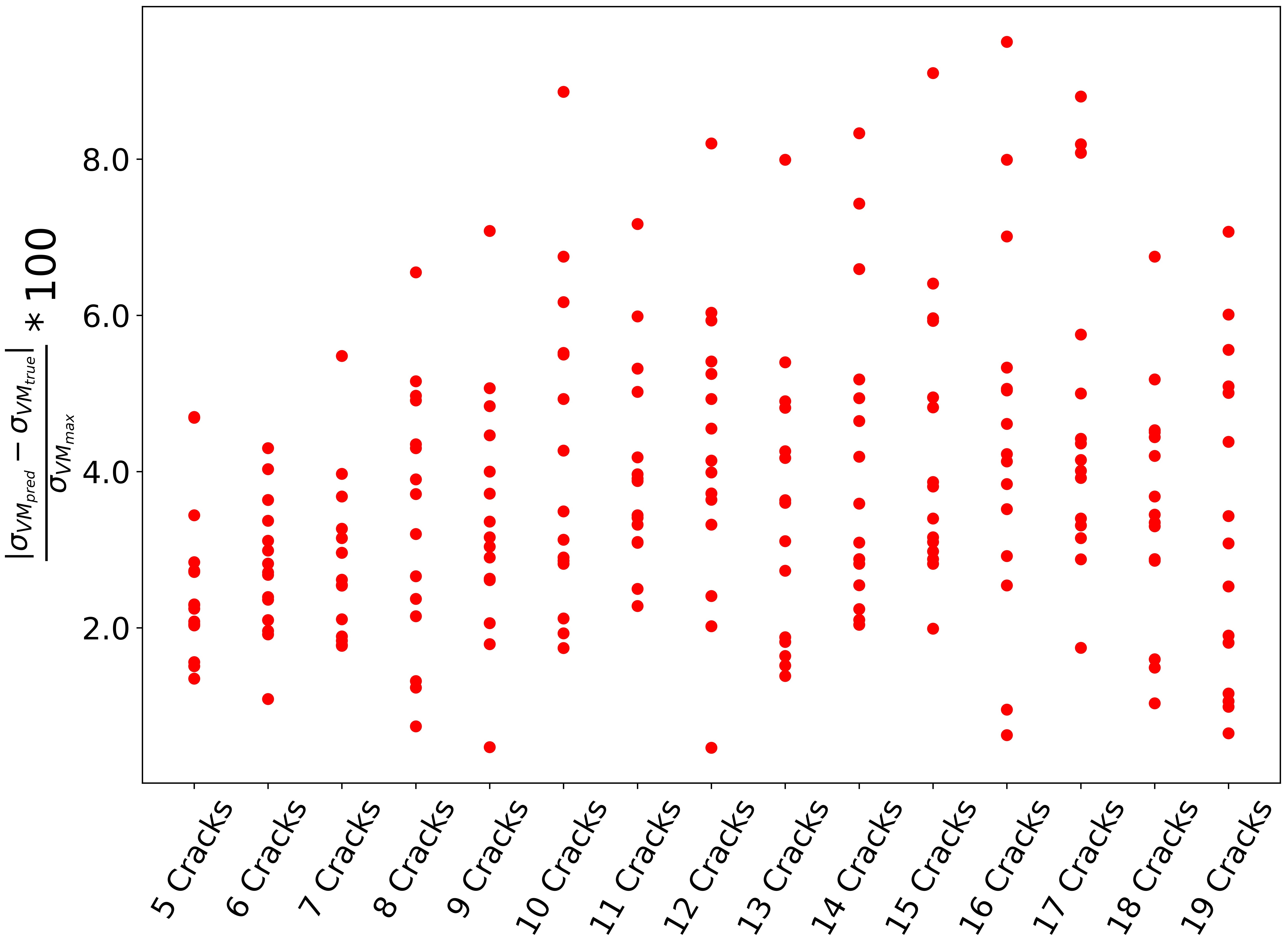


Figure 18 shows that the Microcrack-GNN framework generated errors above in cases involving 10, 12, 14, 15, 16, and 17 microcracks. To understand the origin of these high errors, we look at Figure 19 showing the maximum percentage error of Von Mises stress at each time-step for test case 6 of 16 microcracks. We chose this test case as it showed the highest percent error of Von Mises stress () from the entire dataset as shown in Figure 18. From Figure 19, we see that the maximum percent error stays below error throughout the majority of the simulation. However, at approximately time-step 47 the error increases rapidly above error and reaches its peak of error at time-step 49. Figure 20 shows the Von Mises stress distribution for this test case at time-step 49 (where maximum error occurs) resulting from the XFEM-based model (left-most), the Microcrack-GNN framework (center), and the absolute error between the two (right). The source of error can be seen to originate from the stress intensity factors of the cracks coalescing. Therefore, one of the limitations of the developed framework is the high error resulting when two or more cracks coalescence. Since the Von Mises stresses are computed using the predicted Mode-I and Mode-II stress intensity factors, which are then superimposed for all crack-tips in the system, the error adds up. A possible future work to circumvent this challenge is to predict the Von Mises stress directly throughout the mesh.