Thin accretion discs around spherically symmetric configurations with nonlinear scalar fields
Abstract
We study stable circular orbits (SCO) around static spherically symmetric configuration of General Relativity with a non-linear scalar field (SF). The configurations are described by solutions of the Einstein-SF equations with monomial SF potential , , under the conditions of the asymptotic flatness and behavior of SF at spatial infinity. We proved that under these conditions the solution exists and is uniquely defined by the configuration mass and scalar "charge" . The solutions and the space-time geodesics have been investigated numerically in the range , , . We focus on how nonlinearity of the field affects properties of SCO distributions (SCOD), which in turn affect topological form of the thin accretion disk around the configuration. Maps are presented showing the location of possible SCOD types for different . We found many differences from the Fisher-Janis-Newman-Winicour metric (FJNW) dealing with the linear SF, though basic qualitative properties of the configurations have much in common with the FJNW case. For some values of , a topologically new SCOD type was discovered that is not available for the FJNW metric. All images of accretion disks have a dark spot in the center (mimicking an ordinary black hole), either because there is no SCO near the center or because of the strong deflection of photon trajectories near the singularity.
Keywords:
naked singularities, test particle motion, accretion diskspacs
11I Introduction
Scalar field (SF) configurations in General Relativity and its modifications are interesting for several reasons. Various SF models are extensively used in cosmology Copeland et al. 2006; Bamba et al. 2012; Novosyadlyj et al. 2015; Linde 2014. Some propositions to relax the well-known "Hubble tension" involve SF in diverse approaches to dynamical dark energy (see Valentino et al. 2021 for a review). It is currently unknown, whether the cosmological fields of the late epoch (if any) are the same as the fields that caused the early inflation, or they are of a completely different nature. In any case, the question arises about possible manifestations of SF in relativistic astrophysical objects. Interest in alternative models of these objects has increased significantly after the image of the accretion disk in the core of M87 had been obtained with the Event Horizon Telescope (EHT) Collaboration 2019, demonstrating future prospects to distinguish the black holes from their exotic mimickers.
The first example of the static spherically symmetric solution of Einstein equations with linear massless SF has been found by Fisher Fisher 1948 and later, in the other form, by Janis, Newman & Winicour Janis et al. 1968 (hereinafter FJNW solution; see also Wyman 1981; Virbhadra 1997). The FJNW metric does not describe a black hole (BH), it has naked singularity (NS) in the center not hidded by an event horison. This is a typical feature of static solutions with SF describing compact objects due to the Bekenstein theorems Bekenstein 1972a; Bekenstein 1972b, see also a generalisation in case of multiple SFs Doneva and Yazadjiev 2020. The occurrence of NS in the real Universe is forbidden by the Penrose Cosmic Censorship hypothesis Penrose 1965; Penrose 2002; though, the question on the validity of this hypothesis remains open Christodoulou 1984; Ori and Piran 1987; Joshi and Dwivedi 1993. Current discussions on this topic have shifted to issues of stability and realistic choices of initial data for the gravitational collapse that may or may not lead to NS (see, e.g., Ong 2020 for a review).
Anyway, the final answer regarding the role of SF in astrophysics must be based on observations. It should be noted that there are "exotic" structures Olivares et al. 2020; Aelst et al. 2021; Herdeiro et al. 2021; Abdikamalov et al. 2019; Banerjee et al. 2020a; Banerjee et al. 2020b; Sau et al. 2020; Vincent et al. 2021, which mimic the BHs yielding image similar to that observed by EHT Collaboration 2019. New theoretical efforts as well as observations with better resolution are mandatory. Given the progress in astronomical technology, it is important to study in detail the properties of relativistic astrophysical objects, which can help to select the appropriate options from a variety of theoretical models. The main source of observational information from these objects is associated with the distribution of surrounding radiating matter (accretion disks, jets etc) and images of this matter seen by a distant observer. The very first step is to study stable circular orbits (SCO) of test bodies and their distribution in gravitational field of the configuration. There are a number of papers on this subject including those, which use FJNW solution dealing with the linear SF Bambhaniya et al. 2019; Sau et al. 2020; Shaikh and Joshi 2019; Gyulchev et al. 2019; Gyulchev et al. 2020; Chowdhury et al. 2012; Zhou et al. 2015 and it would be interesting to study effects of nonlinearity. Several examples Pugliese et al. 2011; Pugliese et al. 2013; Slaný and Stuchlík 2020; Stuchlík and Schee 2015; Dymnikova and Poszwa 2019; Vieira et al. 2014; Stashko and Zhdanov 2018; Meliani et al. 2015; Chowdhury et al. 2012 demonstrate occurrence of circular orbit distributions with several non-connected rings of SCO. This may be of particular interest as observational signs of differences from ordinary black holes, as well as the unusual form of the accretion disk images and/or their radiation properties Stuchlík and Schee 2014; Schee and Stuchlík 2016; Stuchlík et al. 2019; Paul et al. 2019; Shahidi et al. 2020; Abdikamalov et al. 2019; Collodel et al. 2021; Shaikh and Joshi 2019; Gyulchev et al. 2019; Gyulchev et al. 2020.
In the present paper, we will look for the effects of nonlinear fields on the SCO distribution (SCOD) around the center. For this purpose, we consider SFs determined by a sequence of monomial potentials , , which have a simple asymptotic behavior at large distances (analogous to FJNW)11 1 The cases with lead to asymptotics at infinity different from .. The reason for such choice is that this is the simplest nonlinear generalization of the FJNW problem. On the other hand, the monomial potentials are often used in various cosmological problems (see, e.g., Smith et al. 2020; Antusch et al. 2020; Ballardini et al. 2019) We numerically obtain static solutions of the Einstein-SF equations in the case of spherical symmetry and use these results to study SCO with focus on the qualitative features of SCOD, as well as on images of these distributions that can be observed from infinity. Namely, we systematically analyse the permitted SCO regions.
The paper is organised as follows. In Section II we write down the basic equations and integrate them numerically. The use of numerical methods presupposes that the problem is well posed. In this regard, we rely on the results of Zhdanov and Stashko 2020, which guarantee that our solutions are regular and they have no singularities outside the center (in contrast, e.g., to some special relativistic cases Zhdanov and Stashko 2020). Also, in Appendix A we prove that there is a unique solution defined by the boundary conditions at infinity. In Section III we proceed to test particle motion in the gravitational field of the configuration. the "equatorial" plane and present possible SCOD. Four qualitatively different SCOD types are introduced, differing in the number of individual SCO rings (subsection III.2). Here we demonstrate how the topology of the SCO rings change with and present maps that define types of SCOD for given configuration parameters. The next subsection III.3 discusses photon trajectories that are used to build the images of different SCOD. The concluding remarks are summarized in Section IV where we discuss observational signatures of SCOD, which can be used to distinguish them.
II Spherically symmetric static solutions of Einstein relations with scalar field
The general metric of a static spherically symmetric space-time in the "curvature" coordinates (Schwarzschild-like) is
| (1) |
where ; radial variable .
We consider one minimally coupled real SF with Lagrangian density
| (2) |
with
| (3) |
where is not necessarily an integer. More general power law potential can be reduced to (3) by rescaling of the variables. Note that for we have the well known FJNW solution. Some results concerning cases can be found in Stephenson 1962; Asanov 1974; Stashko and Zhdanov 2019a; Zhdanov and Stashko 2020.
The Einstein-SF equations are reduced to the following system:
| (4) |
where ,
| (5) |
and
| (6) |
Here are assumed to be functions and is a function for .
We deal with isolated configurations; correspondingly, we impose the asymptotic flatness conditions as follows
| (7) |
where and is the configuration mass; also for and
| (8) |
where parameter defines the strength of the scalar field at spatial infinity; we will call it "scalar charge". Relation (8) yields
The global behavior of the solutions satisfying (7,8) has been studied in a more general case of multiple scalar fields Zhdanov and Stashko 2020, where a proof of regularity of solutions on open interval is given. Asymptotic properties for have been derived in Zhdanov and Stashko 2020 for a particular case, under the assumption that the solutions can be expanded in powers of . In Appendix A of the present paper we provide a more rigorous analysis by means of an iteration procedure. We prove that there is a solution of equations (4, 5, 6) for , where is large enough, with the conditions (8); this solution is uniquely defined by parameters . The first iterations of this procedure yield asymptotic relations for large as follows:
| (9) |
| (10) |
where for and for . Note that in general case (9,10) can contain non-integer powers of .
Asymptotics of the metric near the center can be found in Zhdanov and Stashko 2020: . Parameter characterizes the strength of the singularity. There is a critical point that separates two types of the singularity with different behavior of the null geodesics (see below).
We performed a detailed numerical investigation of the problem (4–8) for , , . To find the solutions for , we proceed numerically starting at sufficiently large initial radius (up to ) to use initial conditions in accordance with asymptotic relations (9, 10). We integrate backwards from higher to lower values of .
The qualitative properties of the metric coefficients and scalar field are rather similar for different values of parameters : is monotonically increasing function bounded from above by 1 for and has a maximum at some point . If increases, then is shifted to larger values and the maximum becomes less pronounced.
The scalar field is always a monotonically decreasing function and as .
For large and fixed , the solutions approach the FJNW curves, except for a small region near the singularity.
An important point is the dependence of upon the parameters of the configuration at spatial infinity. Qualitatively, dependencies for different are rather similar; Fig. 1 shows the examples for and .


III Test particle motion
III.1 General relations
This Section deals with trajectories of the test particles in the space-time corresponding to the solutions of the problem (4–8). The equations of the test particle motion follow from formal Lagrangian
| (11) |
where is a canonical parameter. Standard procedure involves the first integrals for trajectories in the equatorial plane ():
| (12) |
| (13) |
where in case of null trajectories and for the test particles with the non-zero mass; are the integrals of motion. This yields
| (14) |
where .
Thus, we the problem is reduced to investigation of the one-dimensional particle motion in the field of effective potential . The asymptotic behavior of the potential depends on asymptotics (10) at infinity and those near singularity (see Zhdanov and Stashko 2020). For we have
| (15) |
Thus for we have at , i.e. there is an infinite potential barrier that will reflect falling particles. For , at , the particles can approach the center and there is a maximum at some , which is the radius of an unstable circular orbit.
III.2 Circular orbits
We consider the Page-Thorne model of the geometrically thin accretion disk (AD) Page and Thorne 1974, where the averaged motion of accretion matter is approximated by means of SCO around gravitating center. A circular orbit is stable if the right hand side of (14) is zero and changes its sign at this point. For the congruence of circular orbits with different radii in equatorial plane we get dependencies of the specific energy and the specific angular momentum, and the angular velocity upon radius as follows
| (16) |
We use a semi-analytical method of our works Stashko and Zhdanov 2018; Stashko and Zhdanov 2019b to study bifurcations associated with the appearance and disappearance of the minima of . Essentially this is connected with investigation of joint conditions and , which allow us to exclude ; this leads to a necessary condition , where
| (17) |
Using equation (17), we get the bifurcation values and under conditions that and . We tested our results by considering the explicit forms of near the bifurcations as in the example in Fig. 2. The right panel of Fig. 2 illustrates occurrence of three minima (which is not observed in case of FJNW solution); it shows how the shape of the potential changes with increasing the angular momentum, and as a result, the third minimum appears in the vicinity of the singularity. Note that the bifurcation radius (boundary radius), signalizing emergence or disappearance of some minimum of , indicates the boundary of some SCO ring for a given configuration.


The above reasoning allowed us to obtain the boundaries of rings containing SCO, which are separated by regions where circular orbits are either unstable or do not exist. Figs. 3, 4, 5 below present examples of bifurcation curves, which define these boundaries.
Here we describe main results of our numerical investigation of the bifurcation radii , where index denotes various SCOD type explained below. We show that at least four SCOD types are possible in our problem.
The next 3 types deal with the case of (effective potentials are unbounded)
- •
S1: is monotonically increasing function. As a result we have one connected domain of SCO with radii . SCO fill all the space.
- •
S2: The effective potentials have two minima, which correspond to the SCO radii. As a result we have inner disk with SCO radii and outer disk with . Hereinafter, the index in parenthesis denotes the type.
Note that types U1, S1, S2 exist in the FJNW case.
- •
S3: We found a new type of the SCO distribution that does not exist in the FJNW case. The effective potential can have three possible minima and two maxima corresponding to three SCO regions , ,. These regions are separated by two rings of the unstable orbits with , . Fig. 2 shows typical dependencies of and . The emergence of SCO with small radii occurs in a neighborhood of a change in the shape of at values close to 3, where the type of the singularity changes.
If , then effective potential has a maximum for any . There is a region where either there are no circular orbits at all, or they are unstable.
Here we have only one type:
- •
U1 (Schwarzshild-like SCO distribution): effective potential is bounded from above; for and only one minimum can exist. We have one unstable and one stable regions of SCO; the latter for with lower boundary .
Fig. 3 show two illustrative examples of bifurcation radii , means type of SCOD, as a functions of , which realize different SCOD types. Fig. 4 shows essentially the same, but with more complete picture of the bifurcation radii, which illustrates how the curves transform for larger values. Analogous dependencies are shown on Fig. 5 as functions on . Figs. 4 and 5 show how the shape of the curves changes when passes some critical values.
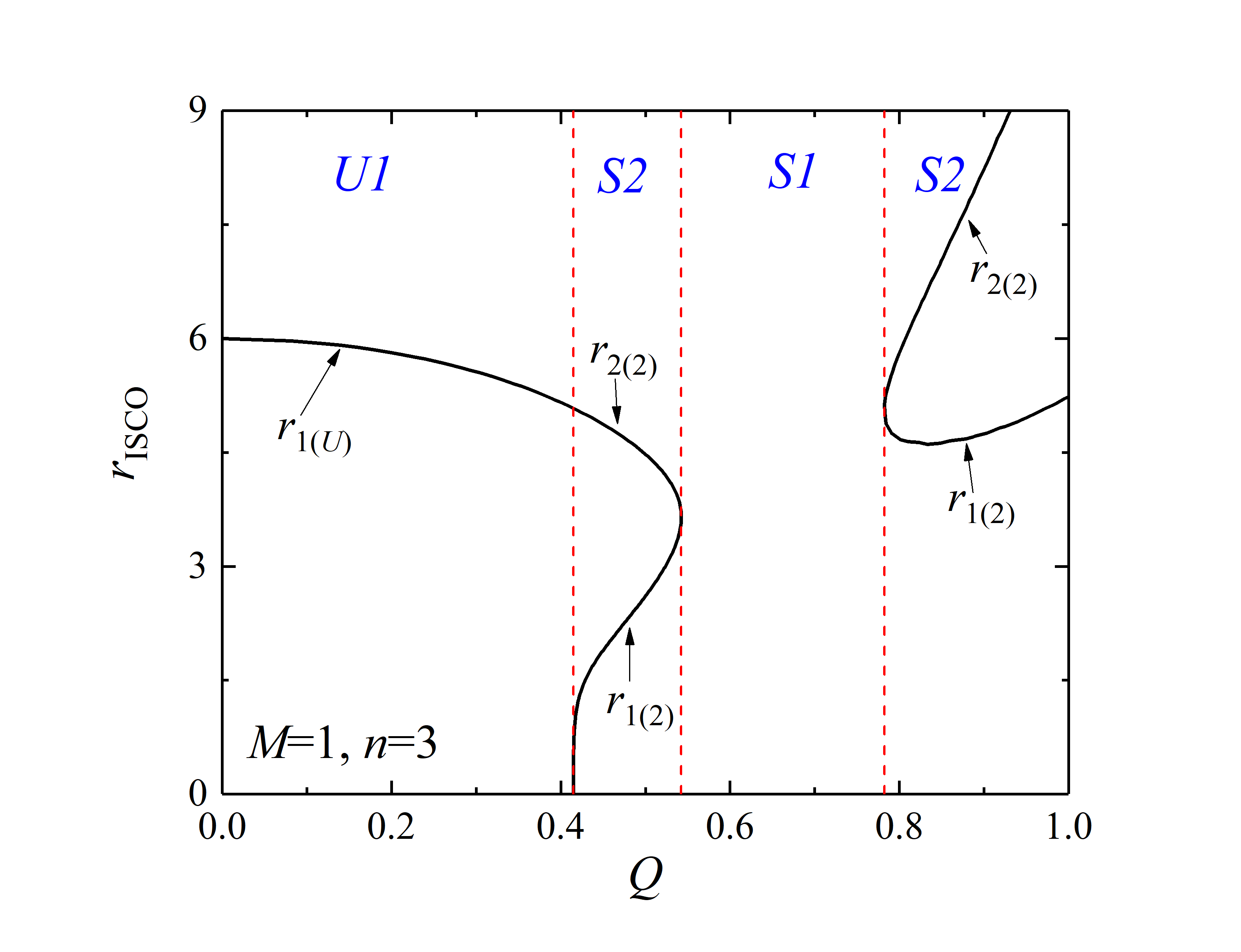

For every there are two branches of the curve (unlike the FJNW case, where there is a single branch exists) and there is a sequence of values , which has the following properties.
- •
The first and the last values denote critical numbers , , which correspond to a reshaping (reconnection) of two branches.
- •
- •
For the right branch moves away to the right and then, for , it starts moving to the left. It is important to note that for moderate , the sizes of unstable regions can be noticeably larger than in the FJNW case.
- •
At , an additional wedge-shaped feature in the left branch appears. This is difficult to show in the right panel of Fig. 4 for , but this is well seen for larger in the right panel of Fig. 3: the corresponding feature is formed by sections and within the area of type. This corresponds to "Pinocchio’s nose" in the right panel of Fig. 5.
- •
For the right branch returns closer enough to the left one and a new area appears. See the right panel of Fig. 3, where there is an additional small area due to the sharp wedge for .
- •
At the tips of the two wedges (see the right panel of Fig. 3) touch each other. The new reshaping of the bifurcation curve occurs, after which the branches reconnect forming a structure represented by the solid curve on the right panel of Fig.4. For large enough , the lower branch tends to the abscissa axis.


We have determined the number of rings with stable and unstable circular orbits and built maps of possible SCODs in the plane for different . Each point on every map (see Figs. 6 – 7) shows the type of SCOD.
For all and there are and types with appropriate . We note that the "thickness" of the ring in the case can be considerably larger than in the FJNW case. The size of area changes non-monotonically: it increases up to and then decreases.
We discovered that the region emerges for (Fig. 6, right); for larger this region becomes to appear for smaller (Fig. 7, right).


III.3 Photon trajectories and accretion disk images
In case of null geodesics (), the effective potential has simple properties. Its asymptotics are due to (15). The sign of is defined by function
| (18) |
We have verified numerically that is a monotonically decreasing function; evidently . For we have if . Therefore, the root of this function can exist only if ; then the point of maximum is a single root of , being the radius of the photon sphere. Fig. 12 shows typical dependencies of the photon orbit‘s radii on the configuration parameters. One can see that is always less than the corresponding radius in Schwarzshild/FJNW cases.


The next step in the study of the configurations in question concerns the images of accretion discs represented by different types of SCOD. In order to build direct accretion disk images, we use the ray-tracing algorithm described in Psaltis and Johannsen 2011; Johannsen and Psaltis 2010; Bambi 2012. The complete consideration of this problem requires knowledge of the brightness distribution of radiating matter over the disk. We have estimated the surface brightness within the Page-Thorne model Page and Thorne 1974 showing the there is a great enhancement of the radiation flux from the innermost region with small radii normalized to the mass accretion rate (analogously to the results of Chowdhury et al. 2012; Gyulchev et al. 2019 on FJNW solution). However, the (unknown) value of may be very different for outer and inner SCO rings and one can expect that the input of the inner ring will be much smaller due to a scattering of the accreting material. This requires a significant modification of the AD model, presumably within the framework of full-scale hydrodynamic modeling, which is beyond the scope of this article. In this view, we limited ourselves to show the observed contours of the SCO regions for accretion disks and the frequency distributions over these disks due to the gravitational redshift and the Doppler effects.
To plot the SCOD images as seen by a distant observer, we need the trajectories of photons falling from infinity. Their properties depend on the sign of . For , when there is maximum of , then the incoming photons with impact parameter , where , will reach singularity at the origin (see the left panel of Fig. 13). For the photons with a nonzero angular momentum will be reflected from the potential (right panel of Fig. 13). Due to the strong bending of the rays, a scattered photon can hit a point on the AD plane far enough from the center, where another photon with a different trajectory also hits. Each such point has two images. On the other hand, there are no photons falling into the AD region near the singularity; this area is not visible to a distant observer.


The photon trajectories needed in the ray-tracing method were obtained numerically, similar to those shown in Fig. 13. We fix a sufficiently large distance to the static observer, where the geometry can be considered flat, and we track the photons coming from the observer to the AD plane, where we take into account only those photons that hit the SCO regions. We do not take into account the input from the reverse side of AD. The frequency ratio between the point at the AD surface and static remote observer for metric (1) is
| (19) |
This formula takes into account both gravitational and Doppler effects. We use the normalized redshift factor
| (20) |
where and is the minimal and maximal frequency ratios on disk, respectively.
Figs. 14–21 show the SCOD contours and the distribution of over the image, visible from infinity. The common feature of all the images is the existence of dark spot in the center like the ordinary black hole. This is either due to the properties of the photon trajectories falling from infinity (, when these photons cannot reach the region near the center), or simply because of absence of SCO in this region.


IV Discussion
We have studied isolated static spherically symmetric configurations of General Relativity with minimally coupled nonlinear SF. The nonlinearity is introduced due to the SF potential . For fixed , we have shown that the solution of the corresponding Einstein-SF system of equations exists and is unique under the appropriate conditions at spatial infinity describing an isolated object. This means that the configuration with scalar field is uniquely defined by two parameters: the configuration mass and the "scalar charge" defined from the SF asymptotics for .
At the center we have a naked singularity with the asymptotic behaviour that involves parameter , which describes the strength of the singularity Zhdanov and Stashko 2020). There is a critical value that separates two types of singularity – attractive and repulsive – with different behaviour of null geodesics near the center.
The solutions of the Einstein-SF system have been investigated numerically up to for sufficiently large and . There are a lot of new elements in comparison with FJNW, which arise in the dependencies of SCOD characteristics on configuration parameters. The most important difference from FJNW is associated with the emergence of the -type of SCOD with two rings of unstable circular orbits for . Indeed, though stable circular geodesics represent the simplified model of an accretion disk Page and Thorne 1974, the above stability properties can be important for real AD.
In general, there are 4 possible SCOD types, the first three being similar to FJNW case. The type is similar to the SCO distribution in the case of the Schwarzschild metric: there is an inner region around the center where circular orbits are either do not exist or are unstable, and there is an outer region of SCO that extends to infinity. For type, SCO fill all the space starting from the center. For type the stable orbits near the center are separated by a ring of unstable orbits from the outer SCO region that extends to infinity. Correspondingly, the images of the thin accretion disks are qualitatively similar to the FJNW case. And, at last, there is a new type () with an additional SCO region and with two rings of the unstable circular orbits that separate SCO rings. Possible cases of SCOD are presented on Figs. 6, 7 for different domains on the plane of the configuration parameters . One can infer that the type is less probable, moreover the innermost SCO rings typically have rather small radii for moderate .
We plotted the observable contours of the accretion disks of the same radius and images of SCO regions using the ray-tracing algorithm Psaltis and Johannsen 2011; Johannsen and Psaltis 2010; Bambi 2012. Figs. 14–21 also show the redshift distribution over AD image, which may be useful to study deformation of the relativistic lines (e.g., Fe K) in the X-ray spectra of compact objects. A common feature of all the images is the dark spot in the center. This is either due to the absence of SCO near the center, or because strong bending of the photon trajectories near the naked singularity. In case of and types, Figs. 16–21 demonstrate features around the center that are not observed for M87* shadow Collaboration 2019. Apparently, these types should be ruled out in case of this object, though observations with better resolution are desirable to have a final answer.
To sum up, we note that basic qualitative properties of static spherically symmetric solutions of the Einstein-SF equations with monomial potential (3) have much in common with the FJNW case Fisher 1948; Janis et al. 1968. However, there are subtle details in the distribution of matter around the configuration, which distinguish the nonlinear SF.
Acknowledgements.
O.S.S. and V.I.Z. acknowledge the support from National Research Foundation of Ukraine (project No. 2020.02/0073). The work of A.N.A. has been supported by a scientific program “Astronomy and space physics” of Taras Shevchenko National University of Kyiv (Project No. 19BF023-01).References
- Copeland et al. (2006) E. J. Copeland, M. Sami, and S. Tsujikawa, International Journal of Modern Physics D 15, 1753 (2006), arXiv:hep-th/0603057 [hep-th] .
- Bamba et al. (2012) K. Bamba, S. Capozziello, S. Nojiri, and S. D. Odintsov, Astrophysics and Space Science 342, 155–228 (2012).
- Novosyadlyj et al. (2015) B. Novosyadlyj, V. Pelykh, Y. Shtanov, and A. Zhuk, Dark energy and dark matter in the Universe, Vol.1: Dark Energy: Observational Evidence and Theoretical Models. Ed. V. Shulga. (2015) arXiv:1502.04177 [astro-ph.CO] .
- Linde (2014) A. Linde, (2014), arXiv:1402.0526 [hep-th] .
- Valentino et al. (2021) E. D. Valentino, O. Mena, S. Pan, L. Visinelli, W. Yang, A. Melchiorri, D. F. Mota, A. G. Riess, and J. Silk, (2021), arXiv:2103.01183 [astro-ph.CO] .
- Collaboration (2019) E. H. T. Collaboration, The Astrophysical Journal 875, L1 (2019).
- Fisher (1948) I. Z. Fisher, Zh. Exp. Theor. Phys., 18, 636 (1948), arXiv:gr-qc/9911008 [gr-qc] .
- Janis et al. (1968) A. I. Janis, E. T. Newman, and J. Winicour, Phys. Rev. Lett. 20, 878 (1968).
- Wyman (1981) M. Wyman, Phys. Rev. D 24, 839 (1981).
- Virbhadra (1997) K. S. Virbhadra, International Journal of Modern Physics A 12, 4831–4835 (1997).
- Bekenstein (1972a) J. D. Bekenstein, Physical Review Letters 28, 452 (1972a).
- Bekenstein (1972b) J. D. Bekenstein, Physical Review D 5, 1239 (1972b).
- Doneva and Yazadjiev (2020) D. D. Doneva and S. S. Yazadjiev, Physical Review D 102 (2020), 10.1103/physrevd.102.084055.
- Penrose (1965) R. Penrose, Physical Review Letters 14, 57 (1965).
- Penrose (2002) R. Penrose, General Relativity and Gravitation 34, 1141 (2002).
- Christodoulou (1984) D. Christodoulou, Communications in Mathematical Physics 93, 171 (1984).
- Ori and Piran (1987) A. Ori and T. Piran, Physical Review Letters 59, 2137 (1987).
- Joshi and Dwivedi (1993) P. S. Joshi and I. H. Dwivedi, Physical Review D 47, 5357 (1993).
- Ong (2020) Y. C. Ong, International Journal of Modern Physics A 35, 2030007 (2020).
- Olivares et al. (2020) H. Olivares, Z. Younsi, C. M. Fromm, M. De Laurentis, O. Porth, Y. Mizuno, H. Falcke, M. Kramer, and L. Rezzolla, Monthly Notices of the Royal Astronomical Society 497, 521–535 (2020).
- Aelst et al. (2021) K. V. Aelst, E. Gourgoulhon, and F. H. Vincent, ‘‘Orbits and images of cubic galileon black holes,’’ (2021), arXiv:2103.01827 [gr-qc] .
- Herdeiro et al. (2021) C. A. Herdeiro, A. M. Pombo, E. Radu, P. V. Cunha, and N. Sanchis-Gual, Journal of Cosmology and Astroparticle Physics 2021, 051 (2021).
- Abdikamalov et al. (2019) A. B. Abdikamalov, A. A. Abdujabbarov, D. Ayzenberg, D. Malafarina, C. Bambi, and B. Ahmedov, Physical Review D 100 (2019), 10.1103/physrevd.100.024014.
- Banerjee et al. (2020a) I. Banerjee, S. Chakraborty, and S. SenGupta, Physical Review D 101 (2020a), 10.1103/physrevd.101.041301.
- Banerjee et al. (2020b) I. Banerjee, S. Sau, and S. SenGupta, Physical Review D 101 (2020b), 10.1103/physrevd.101.104057.
- Sau et al. (2020) S. Sau, I. Banerjee, and S. SenGupta, Physical Review D 102 (2020), 10.1103/physrevd.102.064027.
- Vincent et al. (2021) F. H. Vincent, M. Wielgus, M. A. Abramowicz, E. Gourgoulhon, J.-P. Lasota, T. Paumard, and G. Perrin, Astronomy & Astrophysics 646, A37 (2021).
- Bambhaniya et al. (2019) P. Bambhaniya, A. B. Joshi, D. Dey, and P. S. Joshi, Physical Review D 100 (2019), 10.1103/physrevd.100.124020.
- Shaikh and Joshi (2019) R. Shaikh and P. S. Joshi, Journal of Cosmology and Astroparticle Physics 2019, 064 (2019).
- Gyulchev et al. (2019) G. Gyulchev, P. Nedkova, T. Vetsov, and S. Yazadjiev, Physical Review D 100 (2019), 10.1103/physrevd.100.024055.
- Gyulchev et al. (2020) G. Gyulchev, J. Kunz, P. Nedkova, T. Vetsov, and S. Yazadjiev, The European Physical Journal C 80 (2020), 10.1140/epjc/s10052-020-08575-7.
- Chowdhury et al. (2012) A. N. Chowdhury, M. Patil, D. Malafarina, and P. S. Joshi, Physical Review D 85 (2012), 10.1103/physrevd.85.104031.
- Zhou et al. (2015) S. Zhou, R. Zhang, J. Chen, and Y. Wang, International Journal of Theoretical Physics 54, 2905–2920 (2015).
- Pugliese et al. (2011) D. Pugliese, H. Quevedo, and R. Ruffini, Physical Review D 83 (2011), 10.1103/physrevd.83.024021.
- Pugliese et al. (2013) D. Pugliese, H. Quevedo, and R. Ruffini, Physical Review D 88 (2013), 10.1103/physrevd.88.024042.
- Slaný and Stuchlík (2020) P. Slaný and Z. Stuchlík, European Physical Journal C 80, 587 (2020).
- Stuchlík and Schee (2015) Z. Stuchlík and J. Schee, International Journal of Modern Physics D 24, 1550020 (2015).
- Dymnikova and Poszwa (2019) I. Dymnikova and A. Poszwa, Classical and Quantum Gravity 36, 105002 (2019).
- Vieira et al. (2014) R. S. Vieira, J. Schee, W. Kluźniak, Z. Stuchlík, and M. Abramowicz, Physical Review D 90 (2014), 10.1103/physrevd.90.024035.
- Stashko and Zhdanov (2018) O. S. Stashko and V. I. Zhdanov, General Relativity and Gravitation 50, 105 (2018).
- Meliani et al. (2015) Z. Meliani, F. H. Vincent, P. Grandclément, E. Gourgoulhon, R. Monceau-Baroux, and O. Straub, Classical and Quantum Gravity 32, 235022 (2015).
- Stuchlík and Schee (2014) Z. Stuchlík and J. Schee, Classical and Quantum Gravity 31, 195013 (2014).
- Schee and Stuchlík (2016) J. Schee and Z. Stuchlík, Classical and Quantum Gravity 33, 085004 (2016).
- Stuchlík et al. (2019) Z. Stuchlík, J. Schee, and D. Ovchinnikov, Astrophys. J. 887, 145 (2019).
- Paul et al. (2019) S. Paul, R. Shaikh, P. Banerjee, and T. Sarkar, ‘‘Observational signatures of wormholes with thin accretion disks,’’ (2019), arXiv:1911.05525 [gr-qc] .
- Shahidi et al. (2020) S. Shahidi, T. Harko, and Z. Kovács, The European Physical Journal C 80 (2020), 10.1140/epjc/s10052-020-7736-x.
- Collodel et al. (2021) L. G. Collodel, D. D. Doneva, and S. S. Yazadjiev, The Astrophysical Journal 910, 52 (2021).
- Smith et al. (2020) T. L. Smith, V. Poulin, and M. A. Amin, Physical Review D 101 (2020), 10.1103/physrevd.101.063523.
- Antusch et al. (2020) S. Antusch, D. G. Figueroa, K. Marschall, and F. Torrenti, Physics Letters B 811, 135888 (2020).
- Ballardini et al. (2019) M. Ballardini, D. Sapone, C. Umiltà, F. Finelli, and D. Paoletti, Journal of Cosmology and Astroparticle Physics 2019, 049–049 (2019).
- Zhdanov and Stashko (2020) V. I. Zhdanov and O. S. Stashko, Phys. Rev. D 101, 064064 (2020).
- Stephenson (1962) G. Stephenson, Mathematical Proceedings of the Cambridge Philosophical Society 58, 521–526 (1962).
- Asanov (1974) R. A. Asanov, Theoretical and Mathematical Physics 20, 667 (1974).
- Stashko and Zhdanov (2019a) O. S. Stashko and V. I. Zhdanov, Ukrainian J. Phys. 64(11), 1078 (2019a).
- Page and Thorne (1974) D. N. Page and K. S. Thorne, Astrophys. J. 191, 499 (1974).
- Stashko and Zhdanov (2019b) O. Stashko and V. Zhdanov, Ukrainian Journal of Physics 64, 189 (2019b).
- Psaltis and Johannsen (2011) D. Psaltis and T. Johannsen, The Astrophysical Journal 745, 1 (2011).
- Johannsen and Psaltis (2010) T. Johannsen and D. Psaltis, Astrophys. J. 718, 446 (2010), arXiv:1005.1931 [astro-ph.HE] .
- Bambi (2012) C. Bambi, The Astrophysical Journal 761, 174 (2012).
- Alexandrov et al. (2019) A. Alexandrov, O. Stashko, and V. Zhdanov, Bulletin of Taras Shevchenko National University of Kyiv Astronomy 59, 6 (2019).
Appendix A Iteration method for solutions at large distances
A consideration of existence and uniqueness for an isolated configuration in the asymptotically flat space time has been carried out in our paper Alexandrov et al. 2019, where we have used the so called "quasi-global" coordinates. Here we present a direct proof in the coordinate system defined by the metric representation (1).
We introduce variables
The asymptotic flatness conditions (7,8) can be rewritten in terms of as
| (21) |
From (8) we also have
then
| (22) |
Einstein equations (4,5) and SF equation (6) can be rewritten in terms of as the first order system.
| (23) |
| (24) |
In equation (5) that takes the form
we separate out the dominating term for :
| (25) |
where
| (26) |
In the equation for , which is expressed by means of ,
we also separate out the dominating term:
| (27) |
where
Consider set of continuous vector-functions satisfying
| (28) |
where will be further assumed to be sufficiently large.
We shall construct a system of integral equations for solutions from , which is equivalent to equations (eqs. 23, 25, 24 and 27) with conditions (21). For the estimates below, it is essential that ; the case needs a separate consideration22 2 This can be done in a similar way, but more cumbersome. not presented here.
| (29) |
where we take into account ;
| (30) |
| (31) |
| (32) |
Here integral operators are defined on .
Let . Denote
| (33) |
For sufficiently large , simple estimates on account of (28) and yield
| (34) |
Here and below are finite positive constants. For sufficiently large inequalities (28,34) yield ; whence .
Now we denote
| (35) |
Note that here we use instead of and correspondingly from (33) instead of , which modifies the iteration scheme below. This provides some technical convenience in view of the specific form of the equations involved and allows us to avoid more stringent assumptions on . Using (28,34), for we have
| (36) |
and
| (37) |
where is defined immediately after formula (10).
Whence, for a sufficiently large , and that is . Therefore, we have mapping defined by (33,35), which transforms vector-function
i.e. (for sufficiently large ), operator is correctly defined and maps functional class into itself. Thus, initial equations are reduced to operator equation .
Now we proceed to estimate contraction mapping properties of . Let , ; ; .
Denote
| (38) |
Equations (33) on account of (28) yield
| (39) |
| (40) |
Here and below we systematically use the Lagrange finite-increments formula. Using explicit form (26) of we have
After substitution on account of (39,40) we have
whence
| (41) |
Analogously
then
| (42) |
At last
and we see that, for a sufficiently large , is contraction mapping. The solution can be obtained by successive approximations with zeroth iteration . Leaving the main terms for large , from the first iteration we have
| (43) |
| (44) |
| (45) |
| (46) |
Here we have left those orders in that will not change in subsequent iterations. These equations yield asymptotic relations (9,10).