Hitting Weighted Even Cycles in Planar Graphs

We prove an improved approximation algorithm for ECT in node-weighted planar graphs.

This improves the previously best 10-approximation by Fiorini et al. [11] for planar graphs.

Our algorithm takes as input a node-weighted planar graph $G$ with node weights $c_{v}\in\mathbb{N}$ for each $v\in V(G)$. We then employ a primal-dual algorithm that is based on the following natural covering LP for ECT and its dual, where $\mathcal{C}$ denotes the set of even cycles in $G$:

Fiorini et al. [11] proved that the integrality gap of this LP is $\Theta(\log n)$. Our main result is an improved integrality gap of this LP for ECT in planar graphs:

Designing a primal-dual algorithm is far from trivial, as the imposed parity constraints rule out a direct application of the framework proposed by Goemans and Williamson [14]. Unlike in their work, face-minimal even cycles (even cycles containing a minimal set of faces in their interior) are not necessarily faces, and may thus overlap. Indeed, increasing the dual variables of face-minimal even cycles does not yield a constant-factor approximation in general.

Consider Figure 1, and let $F$ be the inner face that is only incident to blue and black nodes.

For an even number of 5-cycles surrounding $F$, $F$ is the only face-minimal even cycle in the graph. Using only $F$ for the dual increase, even including a reverse-delete step, leaves one blue node of each 5-cycle. Yet, an optimal solution would take a single red and blue node from one 5-cycle.

To circumvent this impediment, we establish strong structural properties of planar graphs related to ECT. Those properties along with results from matching theory allow us to algorithmically find a large set of pairwise face-disjoint even cycles whose dual variables we can then increment. Even with this set of cycles found, it remains technically challenging to bound the integrality gap. For this purpose, we first use the structure of minimal hitting sets of our graph to associate each such set with a hitting set in a subdivision of the so called 2-compression of our graph; the latter is a certain minor that we define in detail shortly. We then show that faces that are contained in even cycles we increment are incident to few nodes on average. Crucial in this step is a technical result that is implicit in the work of Berman and Yaroslavtsev [6]. Eventually, this approach leads to an integrality gap of $47/7$, and an algorithm with the same approximation guarantee.

A block of $G$ is an inclusion-maximal 2-connected subgraph of $G$. The block graph of $G$ is the bipartite graph $B_{G}$ with bipartition $V(B_{G})=B_{1}\cup B_{2}$, where $B_{1}$ are the blocks of $G$, $B_{2}$ are the cut nodes of $G$, and $(b_{1},b_{2})\in B_{1}\times B_{2}$ is an edge if $b_{2}$ is a node of $b_{1}$.

Let $S$ be a partial solution to the given ECT instance at some point during the execution of our algorithm. Then let $G^{S}$ be the corresponding residual graph that we obtain from $G-S$ by deleting all nodes that do not lie on even cycles. Our primal-dual algorithm now first looks for an even cycle $C$ in $G^{S}$ such that at most two nodes of $C$ have neighbours outside $C$. If such a cycle $C$ is found, we increment its dual variable $y_{C}$ until a node becomes tight. The reason for doing this is that such a cycle will pay for at most two hit nodes, which we will show later.

If there is no even cycle $C$ in $G^{S}$ such that at most two nodes of $C$ have neighbours outside $C$, we successively compress the residual graph $G^{S}$ using two types of graph compression. To this end, first note that any minimal solution will only contain one node in the interior of any induced path in $G^{S}$. Suppose we contract some path $P$ of $G^{S}$ of length at least two down to an edge $e$. Choosing a node in the interior of $P$ is “equivalent” to choosing the edge $e$. This is the motivation for the $1$-compression.

Suppose we contract two $u$-$v$ paths $P_{1},P_{2}$ with lengths of different parity down to edges $e_{1},e_{2}$, respectively. We will find it helpful to think of these edges as a single twin edge between $u$ and $v$ whose parity is flexible. This is the motivation for the $2$-compression.

Formally, we will successively compress $G^{S}$ as follows:

• •

  Obtain the $1$-compression $G^{S}_{1}$ of $G^{S}$ by repeatedly folding degree-2 nodes $v$, as long as they exist, which means to delete $v$ and adding the edge $uw$ between its neighbors $u,w$.

• •

  Note that no pair of nodes in $G^{S}_{1}$ is connected by more than two edges. Obtain $\bar{G}^{S}_{1}$ from $G^{S}_{1}$ by replacing each pair of parallel edges by a twin edge. In $\bar{G}^{S}_{1}$, we now once again fold degree-2 nodes as long as those exist. The resulting graph is the $2$-compression $G^{S}_{2}$ of $G^{S}$.

See Figure 2 for examples of 1- and 2-compression of a graph. In the following, we will omit the superscript $S$ from $G_{1}^{S}$, $\bar{G}^{S}_{1}$, and $G^{S}_{2}$ if this is clear from the context. Let $G_{3}$ be obtained from $G_{2}$ by replacing every edge of $G_{2}$ with a path of length two. If a twin edge was replaced, call the two edges of the path added twin edges. By an abuse of notation, we say that a cycle of $G_{1},\ G_{2}$ or $G_{3}$ is even if it contains a twin edge, or if its preimage in $G$ is even.

In the following, we will sometimes call the subgraph $Q$ of $G$ whose contraction yields a subgraph $R$ of $G_{2}$ the preimage of $R$. If $R$ is an edge, call $Q$ a piece, and say $Q$ corresponds to $R$. Furthermore, call $u$, $v$ ends of $Q$ and other nodes of $Q$ internal nodes. If the edge was twin, call the piece twin, otherwise, call the piece single. The blocks of a piece are cycles and paths, and the block graph of a piece is a path. Each cycle of a piece is called an elementary cycle. For an elementary cycle $C$, call its two nodes $u_{C}$ and $v_{C}$ with neighbours outside $C$ branch nodes. Call the two $u_{C}-v_{C}$-paths $P_{1},P_{2}$ in $C$ the handles of $C$, which form the handle pair $(P_{1},P_{2})$. For an illustration, see the red and light blue edges in Figure 2.

The reason for defining $G_{3}$ is that intuitively selecting a node inside a piece corresponds to selecting the edge corresponding to the piece in $G_{2}$. It will be simpler for us if our hitting set consists of only nodes, so we subdivide each edge of $G_{2}$. Suppose that $S$ is the partial (and infeasible) hitting set for the cycles in $\mathcal{C}$ at some point during the algorithm. Further, assume that $G^{S}$ has even cycles, but none with at most two outside neighbours. In this case, one can see that if an even cycle $C^{\prime}$ in $G^{S}$ contains an internal node of some piece $Q$, then $C^{\prime}\cap Q$ is a path between the ends of $Q$. We illustrate this in Figure 3. It follows that $C^{\prime}$ has the form $v_{1}P_{1}v_{2}P_{2}\ldots v_{k}P_{k}v_{1}$, where for $i=1,\ldots,k$ the nodes $v_{i},v_{i+1\mod k}$ are ends of some piece $Q_{i}$, and $P_{i}$ is a $v_{i}$-$v_{i+1}$ path in $Q_{i}$. For $i=1,\dots,k$, the pieces $Q_{i},Q_{j}$ for $i\neq j$ are disjoint except for their ends. We will say that $C^{\prime}$ in $G^{S}$ corresponds to the cycle $C=(v_{1},\ldots,v_{k})$ in $G^{S}_{2}$.

For each such cycle $C$, its blended inequality is

where $a^{C}_{v}\in\{0,1/2,1\}$ for all nodes $v$, and where the support of $a^{C}$ is contained in the node set of the preimage of $C$. We next provide a precise definition of the coefficients of ( ⊛ ‣ 2.1). With those, one can show that ( ⊛ ‣ 2.1) is dominated by a convex combination of inequalities $x(C)\geq 1$ in ( P ECT ).

Consider an elementary cycle of the preimage of $C$ and let $h_{1},h_{2}$ be its two handles. For each of these handles, we define its residual cost as the smallest residual cost of any of its internal nodes. Suppose that the residual cost of $h_{2}$ is at most that of $h_{1}$. We will also call $h_{1}$ the dominant, and $h_{2}$ the non-dominant handle of this cycle. As an invariant, our algorithm maintains that the designation of dominant and non-dominant handles of an elementary cycle does not change throughout the algorithm’s execution.

Suppose first that the residual cost of $h_{1}$ is strictly larger than that of $h_{2}$. In this case, let $a^{C}_{v}=1$ for all internal nodes of handle $h_{1}$, and let $a^{C}_{v}=0$ of the internal nodes of $h_{2}$. If the residual cost of both handles is the same, we let $a^{C}_{v}=1/2$ on internal nodes of both handles.

In certain cases, we need to correct the parity of the constructed inequality. This is necessary if $a^{C}$ as defined above is $0,1$ (i.e., if all elementary cycles of $C$ have a strictly dominant handle), and if the cycle formed by all dominant handles is odd. In this case, we pick an arbitrary elementary cycle on $C$, and declare it special. For this special cycle, we then set $a^{C}_{v}=1$ for the internal nodes on both handles. Following the same reasoning as Fiorini et al. [11] for DHS, we can show the following for ECT:

In our algorithm, we assume that inequalities ( ⊛ ‣ 2.1) are part of ( P ECT ). Throughout the algorithm, we increase dual variables $y_{\circledast}$ of such inequalities.

We will sometimes say that variable $y_{\circledast}$ (or cycle $C$) pays for $\sum_{v\in S^{\prime}}a^{C}_{v}$ hit nodes. It is well-known (see, e.g., Goemans and Williamson [14]) that if during any iteration dual variables for a family of blended inequalities are incremented uniformly, and the dual variables pay for $\alpha$ hit nodes (of $S^{\prime}$) on average, then the final solution produced by the algorithm is $\alpha$-approximate.

The motivation for blended inequalities is to pay for no more than one node in each piece. Consider the example in Figure 1. Here, the bottom black dashed path is odd, there are an even number of handle pairs in the top part, and $\varepsilon$ is small. Suppose we set $a^{C}_{v}=1/2$ on internal nodes of each handle. If we were to increment the inequality ( ⊛ ‣ 2.1), all the blue nodes of weight $1$ would become tight, and after reverse-delete, the algorithm would keep one blue node for each handle pair. However, selecting a red node and a blue node would be a cheaper solution. This could be achieved by setting $a^{C}_{v}=1$ for red and black nodes, and $a^{C}_{v}=0$ on blue nodes, until the residual costs of the red nodes become 1, and afterwards setting $a^{C}_{v}=1/2$ on internal nodes of each handle.

During its execution, the algorithm carefully chooses a family of even cycles $\mathcal{C}$ in $G^{S}_{2}$ and increments the dual variables of certain blended inequalities for each $C\in\mathcal{C}$ until a node becomes tight, or the blended inequality changes; i.e. the residual costs of two handles of a handle pair, which were previously not equal, become equal.

In their primal-dual algorithms for cycle transversal problems with uncrossing property, Goemans and Williamson [14] started with the infeasible “hitting set” $S=\emptyset$. While $S$ is infeasible, the dual variables for faces of the residual digraph that are cycles are incremented. A reverse-delete step is applied at the end. The authors show that tight examples for their algorithm feature so called pocket subgraphs. Not surprisingly, the improved algorithm of Berman and Yaroslavtsev [6] has to pay special attention to these pockets to obtain the improvement in performance guarantee.

The following definition of crossing cycles was elementary to the approach by Goemans and Williamson [14] for cycle transversal problems in planar graphs.

Next, we formally define pockets, and we also introduce the new notion of “pseudo-pockets”, the lack of which will help us “cover” our graph with even cycles.

The $12/5$-approximation algorithm of Berman and Yaroslavtsev [6] for Directed FVS in node-weighted planar digraphs $G$ proceeds roughly as follows.

It starts with the empty hitting set $S=\emptyset$. As long as $S$ is not a hitting set for the directed cycles of $G$, it first looks for a pocket $H$ of the residual digraph $G^{S}$, that is the digraph obtained from $G-S$ by deleting all nodes not on a directed cycle. It then increments the dual variables for the set of face minimal directed cycles of $H$, which happen to be faces. It then adds any nodes that become tight to $S$. Once $S$ is feasible, the algorithm performs a reverse deletion step.

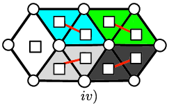
As pointed out, in our setting, face-minimal even cycles may not be faces, and may cross. Following Berman and Yaroslavtsev [6], we wish to “cover” our residual graph with face-minimal even cycles which do not cross, we call this a “tiling”; see Figure 5 iii). As we will see, this tiling allows us to identify the dual variables to increase. Let us formalize the correspondence between edges of the dual between odd faces and even faces.

For a node $v$ of $H^{*}$, let $f_{v}\subset E(H)$ be the edges on the boundary of the corresponding face of $H$. Denote by $h_{\infty}$ the node of $H^{*}$ corresponding to the infinite face.

Given $wh_{\infty}\in E(H^{*})$, a cycle $C^{1}\subset E(H)$ corresponds to $wv_{\infty}$ if $C^{1}$ is a cycle of $f_{w}\Delta f_{h_{\infty}}$, or $C^{1}=C^{\prime}\Delta f_{w}$ and $C^{\prime}$ is a cycle of $f_{w}\Delta f_{h_{\infty}}$. We also call such a cycle $C^{1}$ a tile and say that $C^{1}$ covers $h_{\infty}$, $w$, and the corresponding faces.

Given a matching $E^{\prime}\subset E(H^{*})$ and $V^{\prime}\subset V(H^{*})$, with $E^{\prime}=\{e_{1},\ldots,e_{\ell}\}$ and $V^{\prime}=\{v_{1},\ldots,v_{t}\}$, a set of tiles $\mathcal{T}=\{C_{1},\ldots,C_{\ell+t}\}$ corresponds to $E^{\prime}\cup V^{\prime}$ if $C_{i}$ corresponds to $e_{i}$ for $i=1,\ldots,\ell$ and $C_{j+\ell}$ corresponds to $v_{j}$ for $j=1,\ldots,t$.

In Figure 5 i), cycle $C$ bounds two faces $f$ and $g$; see also Figure 5 ii).

Certain tilings are particularly desirable; we will define these the next.

Let $C$ be an even cycle in $G^{S}_{2}$, and recall that we say that $C$ pays for $\sum_{v\in S}a^{C}_{v}$ hit nodes. For an even cycle in a tiling consisting of two faces, we bound the number of hit nodes it pays for by the number of hit nodes each face pays for.

We will show that a finite face of our graph intersects at most $18/7$ hit nodes on average (over all finite faces). Ideally, we would want to cover all faces by a tiling. Then an even cycle of our tiling is incident to at most $36/7$ hit nodes on average, twice the amount a face of our graph intersects on average. Alas, tilings covering all faces need not always exist. Thus, we try to find a tiling that covers as many finite faces as possible. Suppose that we find a tiling $\mathcal{T}$ that covers a set $\mathcal{T}_{\textsf{Faces}}$ of finite faces consisting of $\alpha$-fraction of the finite faces of our graph. It follows that a face of $\mathcal{T}_{\textsf{Faces}}$ will be incident to at most $18/7\alpha$ hit nodes on average, and so an even cycle of the tiling $\mathcal{T}$ is incident to at most $36/7\alpha$ hit nodes on average. Intuitively, even faces pay for fewer hit nodes than even cycles containing two faces, so it is good if a tiling contains many even faces. The motivation for quasi-perfect tilings is that it is good if a large fraction of faces are covered by the tiling and if the tiling contains a lot of even faces. We prove the following key result in Section 2.6.

We can now formally state our algorithm. It takes as input a planar graph $G$ with cost function $c:V(G)\rightarrow\mathbb{N}$. Let $\mathcal{C}(G)$ denote the set of even cycles of $G$, and let $\mathsf{opt}(G,c)$ denote the minimum cost of an even cycle transversal of $G$, which is a set of nodes intersecting every cycle in $\mathcal{C}(G)$.

As we will see, the algorithm returns an even cycle transversal $S$ of $G$ whose cost is at most $(47/7)\mathsf{opt}(G,c)$. We start with the empty candidate $S:=\emptyset$. In each iteration, the algorithm looks for an even cycle $C$ in the residual graph $G^{S}$ such that at most two nodes of $C$ have outside neighbours. If we find such $C$, increment the variable $y_{C}$ until a node becomes tight. If no such cycle exists, the algorithm computes the 2-compression of $G^{S}$, and in it, we find an inclusion-minimal pocket $H$ of $G^{S}_{2}$. Using Theorem 3, we find a $2/3$-quasi-perfect tiling $\mathcal{T}_{H}$ of $H$ and increments the dual variables for the blended inequalities for each $C\in\mathcal{T}_{H}$. The algorithm then adds all nodes $X$ that became tight to our candidate hitting set $S$.

During an iteration, for each handle pair $(Q_{1},Q_{2})$ for which the set $X$ of nodes that became tight contains a node in the interior of each handle, our algorithm will choose two nodes $a,b\in X$ with $a$ in the interior of $Q_{1}$ and $b$ in the interior of $Q_{2}$ and define $(a,b)$ to be a node pair. For instance, in Figure 2 if $v$ and $v^{\prime}$ are the only nodes added during some iteration then the algorithm would define $(v,v^{\prime})$ to be a node pair. For a set of nodes $X$ added during the same iteration, nodes in a pair are considered to be added before any node not in a pair.

At the end of the algorithm, we perform a non-trivial reverse-delete procedure. Formally, let $w_{1},\ldots,w_{\ell}$ be the nodes of $S$ in the order they were added to $S$ by the algorithm, where for nodes $w_{i},w_{j}$ that were added during the same iteration if $w_{i}$ is in a pair and $w_{j}$ is not, then $i<j$. That is, for reverse-delete purposes, nodes not in a pair are considered for deletion first. For $p=\ell,\ell-1,\ldots,1$, if $w_{p}$ is not in a node pair, then if $S\backslash\{w_{p}\}$ is a feasible ECT, the algorithm deletes $w_{p}$ from $S$; otherwise, it does not. If $w_{p}$ is in a node pair $(w_{p},w^{\prime})$, then if $S\backslash\{w_{p},w^{\prime}\}$ is a feasible hitting set, then delete both $w_{p},w^{\prime}$ from $S$; else, keep both $w_{p},w^{\prime}$.

The intuition behind the caveat in our reverse-delete step is that node pairs are often very useful to keep, because they disconnect a piece. Consider the example in Figure 6.

There is a piece with green nodes of cost $2$, and an odd number of length-5 faces with red and blue striped nodes of cost 1. The black nodes have cost infinity. The bottom dashed path has odd length. In the 2-compression, all length-5 faces in the figure belong to one piece. Suppose for the blended inequality we choose the length-5 face with the green nodes as the special cycle, and we increment this blended inequality. One sees that the red, blue striped and green nodes become tight simultaneously.

To see that reverse delete orders need to be chosen carefully, consider the following adversarial ordering: in reverse delete, consider the two green nodes other than $v$ first, then consider the red nodes, and then consider one blue striped node on each handle. Finally, consider the remaining blue striped nodes. One can see that the algorithm would end up with $v$ and one blue striped node per handle, which is significantly more costly than the optimum which selects the solution consisting of one red and one blue striped node on a handle pair. This completes the description of our approximation algorithm for ECT, whose complete pseudo-code is given as Algorithm 1.

We claim that the algorithm is a $47/7$-approximation for ECT on node-weighted planar graphs.

Fix an input planar graph $G$ with node costs $c_{v}\in\mathbb{N}$. Consider a set $S\subseteq V(G)$ of nodes and a node $v\in S$. A cycle $C$ is a pseudo-witness cycle for $v$ with respect to $S$ if $C\cap S=\{v\}$. If $C$ is additionally even, then $C$ is a witness cycle for $v$. Note that if $S$ is an inclusion-minimal ECT for $G$, then there is a set $W_{v}$ of witness cycles for each node in $v\in S$. If the reverse-delete procedure does not delete any node of $S$, then each node not in a pair has a witness cycle and for each pair, at least one of the nodes in the pair has a witness cycle.

The analyses of the algorithms by Goemans and Williamson [14], and by Berman and Yaroslavtsev [6], for Subset FVS on planar graphs rely crucially on the fact that, each node of an inclusion-wise minimal solution has a witness cycle. Goemans and Williamson [14] showed that one can find a laminar collection $\mathcal{A}$ of witness cycles. Laminar families are well-known to have a natural tree representation. The key argument by Goemans and Williamson [14], and by Berman and Yaroslavtsev [6], is that for each leaf cycle $C$ of the laminar family, one can increment the dual variable of at least one face contained in the region defined by $C$. Further, this dual variable pays only for the hit node that $C$ is a witness of. This is used to argue that a large portion of the dual variables they incremented pay for a single hit node. An additional bound on how many nodes the other dual variables pay for is proven exploiting the sparsity of planar graphs.

For the ECT problem, however, we do not have laminar witness cycles. Instead, we must extend the analysis of Berman and Yaroslavtsev [6] to find a set of laminar pseudo-witness cycles.

Consider some time $\bar{t}$ during the algorithm when applied to $(G,c)$. Let $S_{\bar{t}}$ be the current hitting set and $G^{S_{\bar{t}}}$ the residual graph. Let $\{\sum_{v\in V(G)}a^{C}_{v}\geq 1\}_{C\in\mathcal{L}}$ be the set of inequalities of the increased dual variables. Here, $\mathcal{L}$ will be either a single cycle of $G^{S_{\bar{t}}}$, or a tiling of $G^{S_{\bar{t}}}_{2}$. We wish to show that the primal increase rate towards the final set $S^{\prime}$ at time $\bar{t}$, $\sum_{C\in\mathcal{L}}\sum_{v\in S^{\prime}}a^{C}_{v}$ is at most $47/7$ times the dual increase rate $|\mathcal{L}|$.

If the algorithm incremented $y_{C}$, where $C$ was a cycle of $G$ for which at most two nodes have outside neighbours, then the inequality we increase is $\sum_{v\in C}x_{v}\geq 1$. As $S^{\prime}$ is minimal under reverse-delete, $|C\cap S^{\prime}|\leq 2$, and hence the primal increase rate $\sum_{v\in S^{\prime}}a^{C}_{v}=|C\cap S^{\prime}|$ is at most twice the dual increase rate 1.

Otherwise, if the algorithm did not increment $y_{C}$, then there is no cycle $C$ of $G^{S_{\bar{t}}}$ such that at most two nodes of $C$ have neighbours outside $C$. Hence, the set of increased inequalities are the blended inequalities of a tiling $\mathcal{T}_{H}$ of an inclusion-minimal pocket $H$ of  $G^{S_{\bar{t}}}_{2}$. For a cycle $C$ of $G^{S_{\bar{t}}}_{2}$, let $\sum_{v\in V(G^{S_{\bar{t}}})}a^{C}_{v}\geq 1$ be the blended inequality $C$ (see Equation  ⊛ ).

Recall that informally speaking, we wish to pay for at most one hit node inside a piece. To do this, we need the following theorem which generalizes a result by Fiorini et al. [11, Theorem 5.7] and tells us the structure of a minimal solution within a piece.

Given a hitting set $S^{\prime}$ output by Algorithm 1, we wish to construct a corresponding hitting set for $G^{S_{\bar{t}}}_{3}$ such that the primal increase rate of any particular blended inequality (with respect to $S^{\prime}$) is equals the number of nodes of $S^{\prime}_{3}$ on the corresponding cycle of $G^{S_{\bar{t}}}_{3}$.

To show that $|C_{3}\cap S^{\prime}_{3}|+1$ is small on average we need the fact that $S^{\prime}_{3}$ is a minimal ECT, which is stated in the following remark.

For a node $h$ and cycle $C$, denote by $C\circ h$ that $h$ lies on $C$.

Given an embedding of $G$ and a set $\mathcal{R}$ of faces of $G$, we can obtain an embedding of $\mathcal{D}_{G}$ by placing a node $v_{M}$ inside the face $R$ for each $R\in\mathcal{R}$. This shows the following observation.

Note that for $\mathcal{R}$ a set of cycles, a cycle $R\in\mathcal{R}$, the number of nodes $|R\cap S|$ that $R$ pays for in the hitting set is the degree of $R$ in the debit graph.

Recall the definition of the Subset FVS problem, which seeks a minimum-weight node set $X$ which intersects all cycles from $\mathcal{C}_{T}$, the collection of cycles in $G$ which contain some node from a given set $T\subseteq V(G)$. Observe that each node of $S^{\prime}_{3}$ has a witness cycle in $G^{S_{\bar{t}}}_{3}$; therefore, it is an inclusion-minimal hitting set for the collection $\mathcal{C}_{T}$ with $T=S^{\prime}_{3}$. Goemans and Williamson [14, Lemma 4.2] showed that any inclusion-minimal hitting set for $\mathcal{C}_{T}$ has a laminar set of witness cycles, which implies that there is a laminar set of pseudo-witness cycles $\mathcal{A}$ for hitting set $S^{\prime}_{3}$.

Applying Proposition 1 to $G^{\prime}=G_{3}$ and $X=T=S^{\prime}_{3}$ implies there is a laminar set $\mathcal{A}=\{A_{x}\mid x\in S^{\prime}_{3}\}$ of cycles satisfying $A_{x}\cap S^{\prime}_{3}=\{x\}$. In other words, $\mathcal{A}$ is a laminar set of pseudo-witness cycles for $S^{\prime}_{3}$. Note that cycles of $\mathcal{A}$ may not be even, hence they may be pseudo-witness cycles for $S^{\prime}_{3}$, but not necessarily witness cycles for nodes of $S^{\prime}_{3}$.

Recall that, during the current iteration, our algorithm incremented the blended inequalities of the cycles in a $2/3$-quasi-perfect tiling $\mathcal{T}_{H}$ of $H$. Recall $H$ is an inclusion-minimal pocket of $G^{S_{\bar{t}}}_{2}$. By abuse of notation, let $\mathcal{T}_{H}$ be the corresponding cycles of $G^{S_{\bar{t}}}_{3}$. Let $\mathcal{D}$ be the debit graph formed using $G^{S_{\bar{t}}}_{3}$, the cycle set $\mathcal{T}_{H}$ and hitting set $S^{\prime}_{3}$.

Obtain graph $\mathcal{D}^{\prime}$ from $\mathcal{D}$ by replacing each even cycle $C$ containing two faces with the two faces that compose it. To be precise, construct $\mathcal{D}^{\prime}$ by first taking all nodes of $S^{\prime}_{3}$ and all faces of $H$ that lie inside some even cycle of $\mathcal{T}_{H}$ as the vertex set. For each edge $(C,v)\in E(\mathcal{D})$, if the cycle $C$ consist of two faces $f_{1},f_{2}$ add the edges $(f_{1},v)$ and $(f_{2},v)$ to $\mathcal{D}^{\prime}$, otherwise add the edge $(C,v)$ to $\mathcal{D}^{\prime}$ (see Figure 7). Delete isolated vertices from $\mathcal{D}^{\prime}$.

Let $\mathcal{T}_{\textsf{Faces}(H)}$ be the “face nodes” of $\mathcal{D}^{\prime}$. Let $\mathcal{F}_{\textsf{all}(H)}$ denote the finite faces of $H$. Let $\mathcal{F}_{H}$ denote the set of finite faces of $H$ that contain a hit node. Observe that $M\cap S^{\prime}_{3}=\emptyset$ for each $M\in\mathcal{F}_{\textsf{all}(H)}\backslash\mathcal{F}_{H}$. Now

The first inequality holds, because for each cycle $C$ consisting of two faces $f_{1}$ and $f_{2}$ we have $|C\cap S^{\prime}_{3}|\leq|f_{1}\cap S^{\prime}_{3}|+|f_{2}\cap S^{\prime}_{3}|$. The second inequality holds, because each face of $\mathcal{F}_{H}$ contains a hit node, and so $|C\cap S^{\prime}_{3}|\geq 1$ for each $C\in\mathcal{F}_{H}$. The last inequality holds, because by definition $|M\cap S^{\prime}_{3}|=0$ for all $M\in\mathcal{F}_{\textsf{all}(H)}\backslash\mathcal{F}_{H}$.

If our tiling covers $2/3$ of all finite faces, then $|\mathcal{T}_{\textsf{Faces}(H)}|\leq 2|\mathcal{T}_{H}|$ and $(2/3)|\mathcal{F}_{H}|\leq|\mathcal{T}_{\textsf{Faces}(H)}|$, so $|\mathcal{F}_{H}|\leq 3|\mathcal{T}_{H}|$. Alas, one can show that a tiling that covers $2/3$ of all finite faces does not always exist; see Figure 8.

To overcome this impediment, we will show that $|\mathcal{F}_{H}|\leq 3|\mathcal{T}_{H}|$ holds for a $2/3$-quasi-perfect tiling. Suppose that our $2/3$-quasi-perfect tiling covers a $b$-fraction of the odd faces in $\mathcal{F}_{H}$, and a $c$-fraction of the faces in $\mathcal{F}_{H}$ which are even. Let $\mathcal{F}_{\textsf{even}(H)}$ be the even finite faces of $\mathcal{F}_{H}$. Then, as $\mathcal{F}_{H}\backslash\mathcal{F}_{\textsf{even}(H)}$ are the odd faces of $\mathcal{F}_{H}$, and $\mathcal{T}_{\textsf{Faces}(H)}\backslash\mathcal{F}_{\textsf{even}(H)}$ are the odd faces covered by our tiling, it holds that $b|\mathcal{F}_{H}\backslash\mathcal{F}_{\textsf{even}(H)}|=|\mathcal{T}_{\textsf{Faces}(H)}\backslash\mathcal{F}_{\textsf{even}(H)}|$. Simplifying, we get

References

- Agarwal et al. [2005] A. Agarwal, M. Charikar, K. Makarychev, and Y. Makarychev. approximation algorithms for min uncut, min 2CNF deletion, and directed cut problems. In Proc. STOC 2005, pages 573–581, 2005.
- Bafna et al. [1999] V. Bafna, P. Berman, and T. Fujito. A 2-approximation algorithm for the undirected feedback vertex set problem. SIAM J. Discrete Math., 12:289–297, 1999.
- Baker [1994] B. S. Baker. Approximation algorithms for -complete problems on planar graphs. J. ACM, 41(1):153–180, Jan. 1994.
- Bateni et al. [2011] M. Bateni, M. Hajiaghayi, and D. Marx. Approximation schemes for Steiner forest on planar graphs and graphs of bounded treewidth. J. ACM, 58(5), 2011.
- Becker and Geiger [1996] A. Becker and D. Geiger. Optimization of Pearl’s method of conditioning and greedy-like approximation algorithms for the vertex feedback set problem. Artif. Intelligence, 83(1):167–188, 1996.
- Berman and Yaroslavtsev [2012] P. Berman and G. Yaroslavtsev. Primal-dual approximation algorithms for node-weighted network design in planar graphs. In Proc. APPROX 2012, volume 7408 of Lecture Notes Comput. Sci., pages 50–60, 2012.
- Cohen-Addad et al. [2016] V. Cohen-Addad, E. Colin de Verdière, P. N. Klein, C. Mathieu, and D. Meierfrankenfeld. Approximating connectivity domination in weighted bounded-genus graphs. In Proc. STOC 2016, pages 584–597, 2016.
- Demaine et al. [2004] E. D. Demaine, F. V. Fomin, M. T. Hajiaghayi, and D. M. Thilikos. Bidimensional parameters and local treewidth. volume 18, pages 501–511, 2004.
- Demaine et al. [2014] E. D. Demaine, M. Hajiaghayi, and P. N. Klein. Node-weighted Steiner tree and group Steiner tree in planar graphs. ACM Trans. Algorithms, 10(3), 2014.
- Dorfman and Orlova [1972] Y. Dorfman and G. Orlova. Finding the maximal cut in a graph. Engineering Cybernetics, 10(3), 1972.
- Fiorini et al. [2010] S. Fiorini, G. Joret, and U. Pietropaoli. Hitting diamonds and growing cacti. In Proc. IPCO 2010, volume 6080 of Lecture Notes Comput. Sci., pages 191–204, 2010.
- Fomin et al. [2010] F. V. Fomin, D. Lokshtanov, S. Saurabh, and D. M. Thilikos. Bidimensionality and kernels. In Proc. SODA 2010, pages 503–510, 2010.
- Fomin et al. [2011] F. V. Fomin, D. Lokshtanov, V. Raman, and S. Saurabh. Bidimensionality and EPTAS. In Proc. SODA 2011, pages 748–759, 2011.
- Goemans and Williamson [1998] M. X. Goemans and D. P. Williamson. Primal-dual approximation algorithms for feedback problems in planar graphs. Combinatorica, 18(1):37–59, 1998.
- Hadlock [1975] F. Hadlock. Finding a maximum cut of a planar graph in polynomial time. SIAM J. Comput., 4(3), 1975.
- Karp [1972] R. M. Karp. Reducibility among combinatorial problems. In Complexity of Computer Computations, pages 85–103, 1972.
- Khot and Regev [2008] S. Khot and O. Regev. Vertex cover might be hard to approximate to within . J. Comput. Syst. Sci., 74(3):335–349, 2008.
- Lokshtanov and Ramanujan [2012] D. Lokshtanov and M. Ramanujan. Parameterized tractability of multiway cut with parity constraints. In Proc. ICALP 2012, volume 7391 of Lecture Notes Comput. Sci., pages 750–761, 2012.
- Lokshtanov et al. [2020] D. Lokshtanov, M. Ramanujan, S. Saurab, and M. Zehavi. Parameterized complexity and approximability of directed odd cycle transversal. In Proc. SODA 2020, pages 2181–2200, 2020.
- Misra et al. [2012] P. Misra, V. Raman, M. Ramanujan, and S. Saurabh. Parameterized algorithms for even cycle transversal. In Proc. WG 2012, volume 7551 of Lecture Notes Comput. Sci., pages 172–183, 2012.
- Moldenhauer [2011] C. Moldenhauer. Primal-dual approximation algorithms for node-weighted Steiner forest on planar graphs. volume 222, pages 748–759, 07 2011.
- Nägele and Zenklusen [2020] M. Nägele and R. Zenklusen. A new contraction technique with applications to congruency-constrained cuts. Math. Prog., 183:455–481, 2020.