Multi-wavelength radiation models for low-luminosity GRBs, and the implications for UHECRs2022Multi-wavelength radiation models for low-luminosity GRBs, and the implications for UHECRs–
Abstract
We study the prompt phase of low-luminosity Gamma-Ray Bursts (ll-GRBs) as potential source of very-high-energy (VHE) gamma rays and Ultra-High-Energy Cosmic Rays (UHECRs). Within the internal shock model we choose parameters for the relativistic outflow such that our representative events have observed properties similar to GRBs 980425, 100316D and 120714B and self-consistently calculate the full spectral and temporal properties in a leptonic synchrotron self-Compton scenario. To investigate the conditions under which inverse Compton radiation may lead to a peak in the GeV–TeV range, we vary the fraction of internal energy supplying the magnetic field. Further, we determine the maximal energies achievable for UHECR nuclei and derive constraints on the baryonic loading/typical duration by comparing to the extragalactic gamma-ray background. We find that ll-GRBs are potential targets for multiwavelength studies and in reach for Imaging Atmospheric Cherenkov Telescopes (IACTs) and optical/UV instruments. For comparable sub-MeV emission and similar dynamical evolution of the outflow, weak (strong) magnetic fields induce high (low) fluxes in the VHE regime and low (high) fluxes in the optical. VHE emission may be suppressed by -absorption close to the engine or interactions with the extragalactic background light for redshifts . For UHECRs, the maximal energies of iron nuclei (protons) can be as high as GeV ( GeV) if the magnetic energy density is large (and the VHE component is correspondingly weak). These high energies are possible by decoupling the production regions of UHECR and gamma-rays in our multizone model. Finally, we find basic consistency with the energy budget needed to accommodate the UHECR origin from ll-GRBs.
Keywords:
gamma-ray burst: general – gamma-rays: general – cosmic rays – methods: numerical1 Introduction
During the past two decades the interest in low-luminosity gamma-ray bursts (ll-GRBs) has been rising due to the new observations indicating that these events constitute a sub-population having significantly different characteristics with respect to commonly observed long gamma-ray bursts. In addition, their high local rate (Liang et al. 2007) makes them the key targets for the multimessenger astronomy (e.g. Murase et al. 2006; Boncioli et al. 2019; Liu et al. 2012; Siellez & LIGO Team 2018).
Long GRBs, most probably associated with core-collapse supernovae, typically last 10s of seconds, and are characterized by high isotropic equivalent luminosities, (for a recent review see e.g. Kumar & Zhang 2014). ll-GRBs exhibit substantially lower luminosities , and in some cases substantially longer durations, of up to several seconds Liang et al. 2007; Virgili et al. 2009; Sun et al. 2015. Additionally, these events are characterized by relatively low Lorentz factors during the prompt phase () and lower peak energies (E 100 keV) (Ghirlanda et al. 2018; Cano et al. 2017b).
Due to their low luminosity, ll-GRBs are mostly detected at low redshifts, . Only a small number of ll-GRBs have been observed to date, due to the limited sensitivity of currently running X-ray instruments to low-E events (Liang et al. 2007; Sun et al. 2015). Observations by instruments with the ability to detect very faint GRBs (Foley et al. 2008; Virgili et al. 2009) showed that the population of ll-GRBs is distinct from high-luminosity events, and dominates the local GRB population. It is estimated that the local rate of occurrence of these events is , roughly two orders of magnitude higher than that of high-luminosity GRBs (GRB-HL).
Several interpretations of ll-GRBs have been proposed. One possibility is that they could be accommodated within the same framework as commonly observed long GRBs (having high luminosities), if they were observed off-axis (Pescalli et al. 2015; Aloy et al. 2018). This however implies the existence of a very bright afterglow, which is inconsistent with observations (Daigne & Mochkovitch 2007). Additionally, an off-axis interpretation is not straightforward in various particular cases, given e.g. the chromatic afterglow characteristics (Mandal & Eichler 2010). It has been alternatively proposed that some ll-GRBs are indeed intrinsically less energetic than commonly observed GRBs (Amati et al. 2007). In this case, various scenarios may be invoked to explain the observed emission: one possibility is that of relativistic shock breakouts (Waxman et al. 2007; Nakar & Sari 2012; Bromberg et al. 2011; Nakar 2015). In such cases, jets are choked; they do not penetrate the environment of their progenitors entirely, and instead dissipate their energy into the surrounding medium. Nakar 2015 proposed a unified view, where the differences between common and the low-luminosity events arise from the existence of an extended low-mass envelope in the case of ll-GRBs, in which the jet deposits all of its energy. The observed thermal X-ray emission accompanying the prompt non-thermal emission in several cases can then be interpreted as the breakout of a supernova shock from the effective photosphere of the progenitor star, e.g. Waxman et al. 2007; Sparre & Starling 2012.
Alternatively, collimated emission has also been observed in some ll-GRBs, indicating event topologies similar to those of HL-GRBs, albeit having mildly-relativistic jets (Daigne & Mochkovitch 2007; Ghisellini et al. 2007; Zhang et al. 2012; Irwin & Chevalier 2016). An interesting example is that of GRB 190829A, which was observed at late times during the afterglow phase by H.E.S.S. at very-high ( GeV) energies. For this event, a combination of a shock breakout and a collimated emission episode have been proposed for the prompt phase (Chand et al. 2020). Collimated emission for the prompt phase has also been explored in Fraija et al. 2021; Zhang et al. 2021. This indicates that both the jetted and the breakout physical pictures may be realized in nature, depending on the properties of a particular progenitor.
In this work we explore the possibility that the emission in low-luminosity events can be attributed to intrinsically weak GRB jets seen on-axis. The feasibility of a similar scenario has been discussed for GRB 980425 in Daigne & Mochkovitch 2007 and for GRB 060218 in Irwin & Chevalier 2016, where the prompt X-rays are attributed to a long-lived jet. Unlike these studies, which do not perform time-dependent multiwavelength modelling, we make specific predictions of light curves and spectra.
We model three examples for ll-GRBs with characteristic light curves and emission time-scales, and describe them within the internal shock framework (Daigne & Mochkovitch 1998; Rees & Meszaros 1994; Kobayashi et al. 1997), a multizone model which accounts for different emission sites along the jet. By varying the fraction of energy supplying the magnetic field (thus effectively imposing different magnetic field strengths) and accounting for the corresponding impact on the shape of the predicted spectrum, we study the efficiency of the inverse Compton scatterings at GeV–TeV energies. Our predictions indicate that ll-GRBs are potential targets for the Cherenkov Telescope Array (CTA). We also model the time-dependent evolution of the light curves in different energy bands. We pay special attention to the fluxes in the optical and high-energy regime, which complement the X-ray signatures more commonly observed.
ll-GRBs have also been discussed as a possible population which may power the Ultra-High Energy Cosmic Ray (UHECR) and neutrino fluxes (Murase et al. 2006; Murase et al. 2008; Liu et al. 2011; Murase & Ioka 2013; Fraija 2014; Senno et al. 2016; Zhang et al. 2018; Boncioli et al. 2019). However, Samuelsson et al. 2019; Samuelsson et al. 2020 have argued that cosmic-ray nuclei might not be able to reach utra-high energies required for UHECR fits. These findings were based on the comparison of predicted synchrotron to the observed optical and X-ray flux of a specific GRB. For the theoretical predictions, equipartition parameters (as the fraction of energy transferred to non-thermal electrons) usually found in the literature at face value and an energy budget high enough to power the UHECR flux were assumed (Samuelsson et al. 2020). Additionally, in this (simplified) one-zone model it is assumed that all messengers come from the same region. Investigating the limitations of this approach, we use the multizone results of our radiation modelling to calculate the maximally achievable energies for UHECR nuclei, as well as the implications from the contribution to the Extragalactic diffuse Gamma-ray Background (EGB), such as constraints on the duration versus baryonic loading.
The paper is organized as follows: In Section 2, we introduce our reference events that we select from the list of observed ll-GRBs with confirmed supernova association. Section 3 describes our modelling scheme, and the internal shock model for prompt GRB emission. In Section 3.4 we summarize our (input) assumptions for the modelling used to reproduce the reference events, in Section 4 we derive analytical estimates on the expected luminosity of a high-energy component. The results of our simulations are introduced in Section 5, while we derive the maximal energies attainable for UHECR nuclei in Section 6. The concluding summary can be found in Section 7.
2 Reference GRBs
| GRB | [erg] | [erg/s] | [keV] | [s] | SN | Prototype | |
| 980425 | 34.9 | 0.0085 | 1998bw | sp-GRB | |||
| 031203 | 37 | 0.105 | 2003lw | ||||
| 060218 | 2100 | 0.0335 | 2006aj | ||||
| 100316D | 1300 | 0.0591 | 2010bh | ul-GRB | |||
| 120121B | 18.4 | 0.017 | 2012ba | ||||
| 120422A | 5.4 | 0.283 | 2012bz | ||||
| 120714B | 159 | 0.3984 | 2012eb | hl-GRB | |||
| 130702A | 59 | 0.145 | 2013dx | ||||
| 161219B | 7 | 0.1475 | 2016jca | ||||
| 171205A | 190 | 0.0368 | 2017iuk | ||||
| 190829A | 11 | 0.0785 | 2019oyw | ||||
| 201015A | 10 | 0.426 | AT2020wyy |
The classification of a specific event as a ll-GRB is not always straightforward, primarily due to the difficulty in performing effective followup observations. We list the entire sample of events that, to our knowledge, have been confidently identified as ll-GRBs in Table 1. The sample is restricted to those bursts which have strongly been associated with a known supernova, which supports their interpretation as core-collapse events. We select three events as benchmark scenarios for study, GRB 980425; GRB 100316D; and GRB 120714B. These cases reflect different properties of the known sample of ll-GRBs, such as duration, luminosity, and redshift. The properties of these three events are additionally summarized in Table 2. Our intent is not to reproduce the light curves and spectra of these specific bursts exactly; rather, we use them as characteristic examples of the observed properties of ll-GRBs. The following paragraphs summarize the observations of the selected GRBs. Note that the papers that we will cite in the following do not report the same level of accuracy e.g., for the fitted spectral parameters.
For our first prototype, single-peaked GRB (sp-GRB) we use the observed properties (spectral peak energy, luminosity, redshift, duration, and light curve) of GRB 980425, which has been studied within the internal shock scenario in past studies (see for example Daigne & Mochkovitch 2007 who propose its origin to be a mildly-relativistic low-energy jet instead of a normal GRB being observed off-axis). Given its relatively high peak energy and low isotropic energy, it is an outlier to known GRB correlations (Amati 2006). Its smooth single-peaked light curve makes it a good prototype for studying single light-curve peaks. The time-integrated spectrum has a peak energy of keV Kaneko et al. 2006. The spectral index below the peak is found to be (Frontera et al. 2000) with a peak energy of keV for GRBM (onboard BeppoSAX) observation during the maximum of the pulse, if the spectrum is fit by a Band-function (Band et al. 1993). For an exponential cutoff power-law fit it is determined as with keV, during the maximum of the pulse as observed by BATSE LAD oboard the Compton Gamma-Ray Observatory (CGRO, Kaneko et al. 2006). We additionally summarize the fluences for the various instruments: BeppoSAX reports a fluence of in the 40-700 keV band and in the 2-26 keV range (Pian et al. 2000). Kaneko et al. 2006 performed an analysis of the BATSE LAD observations and fluences of in the X-ray regime (2-30 keV) and a fluence of in the -ray regime (30-400 keV).
Our second prototype, ultra-long GRB (ul-GRB) will have observed properties similar to GRB 100316D, an ultra-long ll-GRB. In contrast to the well-studied ultra-long GRB 060218 (where the black-body component compromises 13 per cent of the prompt spectrum) it has a sub-dominant black-body component contributing only 3 per cent to the the X-Ray flux (0.3 - 10 keV) (Starling et al. 2011). This makes it a suitable candidate for the internal shock model. Also, while GRB 060218 has a very low peak energy of only 5 keV, the peak energy of GRB 100316D is 30 keV. The light curve comprises multiple peaks with maximal photon fluxes decreasing with time. The spectral index below the peak (for a cutoff power-law fit) is found to be (Starling et al. 2011), which is comparable to the one for GRB 060218 (Kaneko et al. 2006 find ). The reported fluence in the Swift BAT range (15-350 keV) is (Starling et al. 2011). The UltraViolet Optical Telescope (UVOT) onboard the Swift satellite reported non-detection in the -band for three different time-intervals (of exposure times 35 s, 194 s and 36 s with mid-times 324 s, 440 s and 634 s after the BAT trigger) Starling et al. 2011. In Fan et al. 2011, these are translated into time-averaged limits between erg/ and erg/, where absorption in our own and the host galaxy are accounted for.
Finally, for our third prototype high-luminosity GRB (hl-GRB) we use the observed properties of GRB 120714B. This GRB has a higher luminosity when comparing it to GRBs 980425 and 100316D, making it a very plausible candidate for an engine-driven scenario (Zhang et al. 2012). The BAT analysis (Cummings et al. 2012) reports a relatively high peak energy of keV and a best fit with a power-law of index . The light curve is simple, single-peaked with =159 s. Being the most distant ll-GRB in our table (), we expect a larger impact of absorption by the Extragalactic Background Light (EBL) on the observed very-high-energy (VHE) spectrum. This burst was observed by Swift BAT, who report a fluence of in the 15-150 keV band Cummings et al. 2012.
3 Multiwavelength time-dependent radiation model

In this section we describe the modelling process, which is divided in several steps illustrated in Fig. 1: We model the evolution of the jet following the internal shock scenario (Daigne & Mochkovitch 1998; Kobayashi et al. 1997). In a similar way as in Daigne & Mochkovitch 2007, we adopted the scenario in which the outflows of LL GRBs are mildly relativistic (having lower bulk Lorentz factors) and have lower wind luminosities. The simulation of the shock dynamics is used to derive the energy dissipated at a certain time and distance from the source, as well as the bulk Lorentz factor of the region. We describe the physical conditions in the shocked medium by three microphysics parameters: the fraction of energy received by non-thermal electrons () and the magnetic field (), and the fraction of accelerated electrons (). With these assumptions we calculate the corresponding spectra in the comoving frame, and convert them into observed quantities. These different steps are described in Sections 3.1–3.3.
3.1 Internal shock model
Here we limit ourselves to a short description of the most relevant formulas while referring to Daigne & Mochkovitch 1998; Bosnjak et al. 2009 for a more detailed view.
A relativistic outflow of a given mass density and velocity profile is approximated by a series of discrete layers with Lorentz factors and masses , separated by a (constant) ejection time , corresponding to our discretization width. From here on we will assume an initially constant wind luminosity of the outflow, given by . This simplified model was validated by the hydrodynamical calculation in Daigne & Mochkovitch 2000; Rudolph et al. 2020. As a fast part of the outflow catches up with a slower one, energy is released in collisions between the layers. The collision between a fast (subscript ) and a slow (subscript ) layer creates a new, merged shell of mass of Lorentz factor
| (1) |
which continues propagating in the outflow and may undergo subsequent collisions.
We assume that during the collision process most of the energy is released as the lighter of the two shells sweeps up a mass comparable to its own; in this case of equal masses of the colliding shells Eq. (1) simplifies to
| (2) |
From energy conservation, the internal energy released during the collision can be calculated as
| (3) |
where is the smaller of the two masses (). Within this model, is the Lorentz factor of the radiation-emitting plasma.
If we define the contrast of Lorentz factors as , we may calculate the comoving mass density and dissipated energy per unit mass during the collision as
| (4) | ||||
| (5) |
where is the distance from the source at which the two shells collide. Primed quantities refer to the comoving frame of the plasma. During the dynamical evolution of the outflow, the distribution of collisions results in a distribution of , and as a function of radius which is fully determined by the initial Lorentz factor distribution and the wind luminosity.
We identify the expansion time (due to adiabatic cooling) as dynamical time-scale of the system for each collision:
| (6) |
Finally, the collision in a GRB of redshift and ocurring at a time (in the source frame) starts to be observed at
| (7) |
3.1.1 Particle acceleration in the shocked medium
In each layer, non-thermal electrons receive the energy , whereas the magnetic field is supplied by a fraction of the internal energy. For the radiation modelling we assume that no baryons are accelerated.
As a pre-set assumption we impose in all collisions and GRBs (as suggested for relativistic shocks).
The relativistic electrons are assumed to follow a power-law of index between a minimum and maximum Lorentz factor (, ):
| (8) |
where is the electron Lorentz factor. In the following, we assume only a fraction of the electrons in the outflow to be accelerated to relativistic velocities and calculate the number of accelerated electrons as . As in Bošnjak & Daigne 2014, we set the fraction of accelerated electrons to be proportional to the dissipated energy per unit mass (via the parameter , ).
Under this assumption, the minimum Lorentz factor of electrons remains constant throughout the evolution and is given by:
| (9) |
This formula demonstrates that the electron spectrum can equivalently described by either or ; we use the latter in this work.
The maximum Lorentz factor is determined balancing radiative losses and acceleration. For this we assume the acceleration time-scale to be defined as
| (10) |
(where is the energy of the particle in the shell frame and the comoving magnetic field strength) as suggested by diffusive shock acceleration and set for electrons.
Synchrotron peak energy and microphysics parameters
The observed synchrotron peak in a single layer is (in the fast-cooling approximation) given by
| (11) |
Given that the magnetic field in the comoving frame can be calculated as , it is straightforward to see that the observed peak depends on both and (under condition that it is not affected by inverse Compton scatterings).
For the reproduction of a given GRB we choose those microphysics parameters such that the synchrotron peak at the maximum of the pulse (the region where most of the energy is dissipated) matches the observed one. For a fixed dynamical jet evolution (setting , , , etc.) this creates a relation between and , leaving only one of them as a free parameter.
3.2 Radiation Modeling
With these assumptions on the accelerated electrons, we calculate the spectrum produced in each layer as a result of the collision occurring between layers of different velocities. These layers correspond to our radiation zone. The overall final spectrum and light curve are given by the superposition of all spectra produced in individual layers, taking into account the time at which collisions occur. Note that the layers are determined by our discretization scheme, and the result does not depend on that as long as enough layers are used and the properties between adjacent layers change slowly enough (compared to the expansion time-scale).
The evolution of the particle spectra and photon fields in each layer are modeled with the time-dependent radiative Code AM3 (Gao et al. 2017) which includes synchrotron radiation, synchrotron self-absorption, inverse Compton scattering in both Thomson and Klein-Nishina regimes, and -absorption. The (low-energy) thermal component is not modeled or taken into account in the current work. As detailed above, the thermal emission (if observed) represents only a small fraction of the energy budget; also its signature might be in any way distinguished from the jetted emission. While some studies (Bosnjak et al. 2009; Bošnjak & Daigne 2014; Globus et al. 2015) neglect the effect of secondary lepton pairs created by -absorption, they are explicitly included in our approach. Being treated the same way as primary leptons, those pairs contribute by synchrotron and inverse Compton radiation (see Appendix C for a detailed discussion). In addition to the effects described above we account for adiabatic cooling due to the expansion of the shell with the cooling time given by . We note that adiabatic cooling is expected to impact the electron spectra mostly in the low-energy ranges (where the contribution to the observed photon spectra is small), representing the longest cooling time-scale of electrons (see Fig. 14).
The initial distribution at of accelerated electrons in the comoving volume is in our model given by Eq. (8) and no further injection of electrons beyond this point is assumed. This means that we do not make any assumptions on how or on what time-scale the radiation zone is filled with electrons, which depends on the details of the acceleration process.
We follow the particle spectra and radiative processes over the dynamical time-scale and take the spectrum at as final, emitted spectrum. Since this represents the slowest cooling time-scale of electrons, at all electrons are expected to have cooled. As an result, they will not contribute anymore to the photon spectrum. This approach also (roughly) corresponds to the assumption of photons escaping over the dynamical/expansion time-scale. However, this treatment is only approximate - with a full treatment of the escape in the radiative calculations (incorporating an escape term of in the partial differential equations and integrating over the escaped spectra), the temporal evolution of the spectra within single layers would also leave an imprint on the observed spectra.
3.3 Conversion to observed spectra and light curves
Given an total energy density of photons (, where is the comoving volume of the emitting layer and is the comoving photon energy), one may compute the differential observed fluence for a single collision as
| (12) |
with the comoving distance .
For the calculation of time-dependent quantities such as the light curves and the time evolution of spectra, we follow Granot et al. 1999 and take into account the curvature of the emitting surface for each collision.
Given our focus on the (expected) high-energy component, we explicitly incorporate absorption due to interactions with the EBL in our simulations which are expected to impact the spectra in the TeV-range for redshifts Abdalla et al. 2017. EBL absorption is calculated using the open-source gammapy package (Deil et al. 2018; Nigro et al. 2019), using the model of Dominguez et al. 2011.
3.4 Parameter space for reference GRBs
| GRB 980425 | GRB 100316D | GRB 120714B | ||
| Observed | [erg] | |||
| [s] | 35 | 1300 | 159 | |
| [keV] | 122 | 30 | 101 | |
| 0.0085 | 0.059 | 0.3984 | ||
| sp-GRB | ul-GRB | hl-GRB | ||
| Input | 40, 10 | 40, 10 | 80, 20 | |
| [erg/s] | ||||
| 1000 | 1000 | 1000 | ||
| [s] | 40 | 1000 | 130 |


| sp-GRB | ul-GRB | hl-GRB | ||||||||||
| [G] | [G] | [G] | ||||||||||
| 7.3 | 3.0 | 5.8 | 820 | 9.2 | 2.8 | 7.6 | 234 | 5.7 | 3.6 | 6.0 | 346 | |
| 4.1 | 5.3 | 3.2 | 257 | 5.2 | 5.0 | 4.3 | 74 | 3.2 | 6.4 | 3.4 | 110 | |
| 2.3 | 9.4 | 1.8 | 82 | 2.9 | 8.9 | 2.4 | 23 | 1.8 | 11.3 | 1.9 | 35 | |
| 1.3 | 16.8 | 1.0 | 26 | 1.6 | 15.9 | 1.4 | 7 | 1.0 | 20.1 | 1.0 | 11 | |
We summarize our assumptions on the initial jet configuration (ejection time and luminosity, Lorentz factor profile) in Table 2, the (initial) Lorentz factor distributions are displayed in Fig. 2. The Lorentz factor distribution, engine active time and wind luminosity are closely related to observations such as the light curve and emitted isotropic energy and thus relatively well constrained. For example, to reproduce a multi-peaked light curve (as the one of GRB 100316D/ul-GRB), also a multi-peaked Lorentz factor distribution is necessary. In accordance with Lorentz factor measurements of ll-GRBs, we choose relatively low Lorentz factors of the outflow. Note that due to their relatively low luminosities, we expect sp-GRB and ul-GRB not to have Thomson optical depths above unity, despite their low Lorentz factors. As hl-GRB has a higher luminosity, we impose higher initial Lorentz factors in this case (see Ghirlanda et al. 2018 for a correlation of GRB Lorentz factors and luminosities). The higher Lorentz factors for this prototype will also ensure the outflow to be optically thin, despite the higher luminosity.
We adjust the fraction of accelerated electrons with such that we can fit the observed peak of the reference event as a synchrotron peak (see Section 3.1 for a more detailed description) and leave as a free parameter to study the impact of the magnetic field strength. The values of and (the maximum value of during the fireball evolution) and the maximum magnetic field for all models and our choices of are summarized in Table 3.

To illustrate the dynamical evolution of the outflow, we show , and as a function of collision radius for sp-GRB in Fig. 3. The evolution of those parameters depends only on the initial Lorentz factor distribution of the outflow and the jet luminosity ; for it is assumed that .
4 Theoretical predictions for the high-energy emission
A significant emission at very high energies from low-luminosity events would make them interesting targets for Imaging Air Cherenkov Telescopes (IACTs). So far, the observational strategy of ground-based gamma-ray experiments has nominally been to follow up detection by X-ray instruments, which have not been very sensitive to ll-GRBs. The upcoming Cherenkov Telescope Array (CTA) will improve on the sensitivity of existing IACTs on short time scales (Fioretti et al. 2021). Correspondingly, it will significantly improve the prospects for serendipitous detection of ll-GRBs. As these events are found at lower redshift, the effect of EBL absorption is less significant. The prospects of detecting GeV–TeV emission from ll-GRBs are therefore relatively high, compared to HL-GRBs.
While we describe the general, theoretical predictions on the shape of the photon spectrum in Appendix A, we here provide estimates for the expected luminosity attributed to the inverse Compton component which will give rise to a HE component by calculating the Compton Y-parameter for characteristic spectral properties of ll-GRBs. For simplicity, we consider the scatterings of electrons having Lorentz factors interacting with photons around the peak of the synchrotron emission. We define the dimensionless quantity to measure if the scatterings occur in Klein-Nishina regime () or in Thomson regime ( ) ( denotes the observed peak of the spectrum). The peak energy of synchrotron emission is dominated by electrons at the minimum of the distribution in the cases we presented, and we assume that the average value Y() can be approximated as (Nakar et al. 2009).
- (a)
Klein-Nishina regime
For the case where electrons with Lorentz factors below cool via inverse Compton process in the Klein-Nishina regime we adopt the following approximate expression for (Duran et al. 2012):(13) We use the following expressions for synchrotron cooling time and for the cooling time due to IC scattering in the comoving frame:
(14) (15) Here the cross-section for inverse Compton scatterings of photons around peak energy is smaller than the Thomson cross section by a factor (Duran et al. 2012). Note that the luminosity (which is derived from the observations) in the expression for is considered as the luminosity of the synchrotron component only. is a numerical factor accounting for the scattering angles ( 0.5, Kumar & Zhang 2014). This leads to the expression:
(16) For the values typical of low-luminosity events (L 1047 erg s-1, E 50 keV and 1), we find
(17) We used the notation .
- (b)
Thomson regime
For Compton scatterings occurring in the Thomson regime, we follow again the simplified procedure as in Duran et al. 2012:(18)
The ratio of luminosities is given by . Note that -pair annihilation may produce a high-energy cutoff in the spectrum, suppressing the inverse Compton component, which is not accounted for in the analytical estimate. When Klein-Nishina effects become important, the cross section for scattering photons gets smaller than the Thomson cross-section, and the scattered photon energy is reduced, which results in .
Motivated by Equations 17 and 18, in the following, for the same assumptions on the properties of the outflow, we keep the peak energy of the spectrum approximately constant and study the effect of the magnetic field on the spectral shape. In our model, the magnetic field changes throughout the dynamical evolution of the jet and is not set directly, but through the magnetic energy density via . For Thomson scattering in fast cooling regime, we can easily relate Y to , Y= , and a more general expression for Y can be found in e.g. Kumar & Panaitescu 2003.
5 Results: simulated spectra and light curves
In this section we present the results of our simulations: the predicted observed time integrated spectra, light curves and time resolved fluxes/fluences for different energy bands. The parameter sets used for sp-GRB, ul-GRB and hl-GRB are motivated by the three real GRBs which guide our simulations. For all GRBs, we explore the impact of the magnetic field strength by varying .
Our models reproduce various observed features of the reference GRBs, such as the light curve structure and the spectral shape. The predictions on the multiwavelength features of the presented models will be possible to test by future facilities. This includes the fluence and flux in different energy bands (including optical and very high energy emission) and a possible delayed onset of the HE component.


The lower panel shows the spectral index of the photon flux (for a power-law shape), where the dashed lines correspond to the synchrotron predictions (, and ) and the solid line indicates the position of maxima/minima of .
5.1 Time integrated spectra
In Fig. 4 we show the time integrated spectra for the benchmark scenarios. The grey bands indicate the energy range of the X-ray instruments used for the initial detection of the reference events. For all GRBs we explore realisations for . The observed sub-MeV peak is generated by synchrotron radiation and fluxes in the regime of the observing instrument are (by construction) comparable. The exception are the simulations obtained for , where the fluxes around the synchrotron peak are much lower than for the other choices of and may be in disagreement with the observed fluxes of the reference events. In principle the fluxes in this case could be enhanced by imposing a higher jet luminosity, however at the cost of a reduced comparability to the other results due to changed dynamical properties of the outflow. We show in Appendix B that for for large parts of the dynamical evolution of the jet, the physical conditions in the shocked plasma correspond to the slow-cooling regime. As this further aggravates the efficiency problem of the internal shock model, we suggest that is not a realistic parameter assumption, and will show the corresponding results in the following only for completeness.
The shape of the spectrum is dominated by three features: At the lowest energies, synchrotron self-absorption results in a depletion of the flux and a spectral break. In the intermediate keV-regime, the observed peak energy is produced by synchrotron radiation. At the highest energies above keV, inverse Compton radiation results in a second spectral peak. The change of magnetic field, determined by , shows up mainly in two points: low values of lead to higher fluxes in the regime above keV and lower fluxes below the synchrotron peak, especially in the optical regime.
The systematic dependence of the high-energy component on matches expectations, as the Compton-Y parameter is inversely proportional to (and thus ) in both Klein-Nishina and Thomson regime (see the approximate formulas Eq. (17) and Eq. (18)). We quantify this behaviour by calculating the ratio of the luminosity in inverse Compton to synchrotron component for sp-GRB: numerical values range between LIC/Lsyn = 0.02 for =10-1 to LIC/Lsyn = 0.08 for =10-4.
The time integration was performed on the duration of energy dissipation process. Thus, the depletion of the flux below the spectral peak in the observed spectrum is attributed to two effects: one is the contribution of the low peak energy spectra generated in the late shocks, and the other one is the effect of IC scatterings occuring in Klein-Nishina regime as shown in Fig. 11 (see also Daigne et al. 2011). As VHE emission might be not be observed due to EBL absorption, the systematic dependence of the optical flux on could play a significant role in constraining the magnetic field and can potentially help with the rejection of models and parameter sets (as recently shown in Samuelsson et al. 2020; Oganesyan et al. 2019). This will however require ll-GRBs to be within the sensitivity range of optical instruments. If we compare the optical flux of ul-GRB to the most stringent UVOT -band limits of erg//s for a duration of 1300 s (see Section 2), we find tension with this limit for all results except . For the least stringent UVOT limit both and are not ruled out. We point out that the UVOT limits were obtained for exposure times much shorter than the burst duration and should be taken cautiously for the scenario of a temporally variable source (as ul-GRB). Additionally, these upper limits depend on the level of absorption in the host galaxy, which is often not well determined. Nevertheless, the results illustrate how optical measurements could potentially constrain parameters of the model.
sp-GRB and ul-GRB are not significantly affected by EBL absorption, due to their low redshifts. This is different for hl-GRB, where we additionally show the un-absorbed spectra as dotted lines (right plot of Fig. 4). In this case, emission above is strongly suppressed. We conclude that events at these redshifts are likely not to be observed in the HE regime.
The lower panels of Fig. 4 show the spectral index of the photon flux. The dashed lines show the synchrotron predictions for the fast-cooling () and slow-cooling low-energy slope () below the spectral peak, in addition to the high-energy spectral index () corresponding to . We find that inverse Compton scatterings in the Klein-Nishina regime affect the low-energy slope : in that case values of up to –1 can be achieved (Daigne et al. 2011); for a detailed discussion of the theoretical predictions of the photon spectral shape see Appendix A. This systematic effect on is common to all benchmark scenarios. As a consequence, may be used to draw (more robust) conclusions on the magnetic field strength/ the equipartition parameter in this framework. As the spectral slope changes as a function of energy, the fit energy range will have a large impact on the fit result – an effect which should be taken into account when comparing these predictions to observed data.
5.2 Time-dependent observational signatures
Multiwavelength observations of GRBs are critical, both for their detection and their subsequent interpretation. In particular, observation of temporal correlations of the emission in different bands mitigates the challenge of detecting the short prompt stage of these events. In order to illustrate the potential for discovery, we present the predictions for the fluxes and fluences in different energy regimes -corresponding to existing and upcoming instruments- as a function of observation time.
As the observed fluences are roughly of the same order of magnitude for the three prototypes (see Section 2), we investigate the discovery potential in different energy bands by calculating the corresponding predicted signals for sp-GRB (Fig. 5).


The top panels indicate optical and UV emission, corresponding to the energy bands observable by survey telescopes, such as ZTF (Bellm et al. 2018) and LSST (Ivezić et al. 2019) (energy band e.g., of the ZTF -band 560 - 730 nm) , or a satellite such as the planned ULTRASAT mission (220 - 280 nm) (Sagiv et al. 2014). The middle panels correspond to energy bands of X-ray and gamma-ray instruments, such as Swift XRT (0.1 - 10 keV) (Burrows et al. 2005), and Fermi GBM(8 keV - 30 MeV) (Meegan et al. 2009) . The ranges presented correspond also roughly to the energy ranges of the upcoming SVOM-mission, which consists of the -ray monitor GRM (30 keV to 5000 keV, Dong et al. 2010), the X-ray to -ray telescope ECLAIR (4 keV to 250 keV, Godet et al. 2014), the soft X-ray telescope MXT (0.2 keV to 10 keV, Perinati et al. 2012) and the optical telescope VT (Wu et al. 2011). The bottom panels represent the sensitivity range of ground-based Cherenkov telescopes.
We show predictions for the observable flux and fluence. The realistic sensitivity of the different experiments is not trivial to estimate, as it depends on multiple factors, such as the period of day over which the event occurs; the pointing of a particular telescope upon receiving an alert, etc. However, it is possible to relate our predictions to the nominal capabilities of relevant instruments. While we account for EBL absorption in the HE regime, the effect of extinction in the host galaxy and our own Galaxy (which is relevant for the optical and UV regime) is not taken into account.
Without extinction we predict for sp-GRB a range of flux in the optical band of within 30 s , which roughly corresponds to an AB magnitude within mag for the -band of ZTF. These prompt optical flashes are therefore within the detection sensitivity of the telescope, which is characterized by a corresponding 30 s limiting magnitude of . Similarly, our predicted UV fluence without extinction corresponds to AB magnitudes, . Such a signal would be detectable with the upcoming ULTRASAT, which has an expected limiting magnitude of (over 5 minute exposures) in the corresponding band. We also point out that the ratio of fluences in the optical and UV band () changes for the different magnetic fields and could be used to discriminate between scenarios: While for we find it drops to for and for .
We predict a fluence of over 40 s in the X-ray regime (Swift XRT; 0.1–10 keV) for the different choices of . For context, Burrows et al. 2005 derive an XRT sensitivity limit of given an exposure of 10 s, well below the required detection threshold of an event such as sp-GRB.
Considering the HE and VHE emission, the upcoming CTA has an expected sensitivity of over s intervals (Fioretti et al. 2021) in the energy ranges we consider. Our predicted fluence for most choices of will therefore be within the detection capabilities of this observatory. For this particular example, resolving the light curve with a ground-based IACT, while challenging, might be possible. However, the nature of the emission at these energies depends strongly on the redshift of the source, given the potential high impact of EBL absorption.

To illustrate this point, we show the predicted spectra as a function of energy for hl-GRB in Fig. 6, assuming the same ll-GRB source to be placed at different redshifts. The Figure shows the observed spectra for each redshift, with and without accounting for EBL absorption. The observed duration scales with (see Eq. (7)), where for we calculate a duration of 150 s. The figure also presents the corresponding differential sensitivity of CTA for 150s intervals. It is defined here as the minimal fluence of a source, in order for it to be detectable with at least significance within a given energy range. The sensitivity is derived for the Northern site of the observatory using the ctools simulation package (Knödlseder et al. 2016). We use instrument response functions optimized for short (30 minutes) observations at zenith angles of . The position of the putative source is displaced by from the centre of the field of view of the instrument.
As one may infer, for redshifts of and , the observable emission above 1 TeV is strongly attenuated. We conclude that for a HE component to be detected, these events should be within redshift, . Fortunately, the expected rate of occurrence of ll-GRBs is relatively higher in the local Universe (Liang et al. 2007).
Even more intriguing is the possibility of exploring the time dependence of the photon rates in the HE and VHE bands. We therefore compare the simulated light curves for sp-GRB, ul-GRB and hl-GRB in Fig. 7 for different HE and VHE -ray bands.


For all models, the general features of the temporal structure of the reference GRB sub-MeV light curve is very well reproduced. A smooth single-peaked temporal profile is predicted for sp-GRB (GRB 980425) and hl-GRB (GRB 120714B), and a multi-peaked light curve with decreasing pulse maximum for ul-GRB (GRB 100316D). While EBL absorption plays no significant role for sp-GRB and ul-GRB, we again see that it suppresses the photon fluxes above 1 TeV by at least two orders of magnitude in the case of hl-GRB. In accordance with Fig. 4 we observe a strong dependence of the HE flux has on the magnetic field strength, where choices of low lead to higher fluxes for all models. This difference becomes especially noticeable above 100 GeV. For all models we notice an early, weak peak in the HE/VHE regime (see also the flux below 7 s in Fig. 5). We attribute this to the reverse shock (in contrast to the forward shock, which produces the main emission in single peaks) passing through the ejecta, but point out that due to its relatively low flux this early peak might not be observed.
It is noteworthy that the HE emission shows a delayed onset with increasing in all scenarios. This is an example of how the different observed light curves may be used to constrain the physical processes at play. The early signal in a single-peaked light curve is related to collisions close to the source. These are subject to strong - absorption, which potentially suppress the HE component (Hascoet et al. 2012; Bustamante et al. 2017). This suppression could potentially be slowed by continuous up-scatterings of photons which contribute to a high energy component. For this, however, relativistic electrons need to be present in the region. As we don’t consider a steady injection term but instead follow a cooling electron distribution, this may be realized if electron cooling time-scales are large. This is the case for low-, where the synchrotron cooling time-scale is long; it is in fact the dominating cooling time-scale for high-energy electrons for low- (see Appendix E.1.) Another way of preventing an early suppression of the HE flux due to absorption may be a continuous injection of accelerated particles (ensuring the continuous presence of relativistic electrons in emission region). The latter could be fueled by either a slow enough acceleration process or by the injection of relativistic electrons from (neighbouring) collisions and plasma layers. While thus for low magnetic fields an early and strong HE-peak ( 10 GeV) is predicted, it will become wider and peak later in time with increasing . The wide peak might be connected to the high(er) efficiency in late collisions further away from the source for high .
Overall, the signals observable in different energy bands can influence the observational strategies for future experiments. For instance, while it may be challenging to detect these events at energies, the emission between 50 GeV and 1 TeV is within the sensitivity window of CTA. Furthermore, one may consider the different predictions, related e.g., to different choices of in different energy bands; these illustrate how observations of the time-structure of ll-GRBs may be used to constrain their physical modelling. Considering our three reference models, it is also interesting to note that our models accommodate a rich phenomenology, which may largely be attributed to the properties of the engine (e.g., the Lorentz factor distribution, engine active time and wind luminosity). Time-resolved observations may therefore serve as a direct probe for properties of the central engine.
6 Implications for the connection to UHECRs and neutrinos
ll-GRBs have been recently studied as the sources of the UHECR nuclei in Zhang et al. 2018, and may even describe the PeV neutrino flux and UHECRs across the ankle simultaneously (Boncioli et al. 2019).
We point out that current IceCube neutrino limits suggest that standard high-luminosity GRBs cannot be sources of UHECR and high-energy neutrinos (Abbasi et al. 2012; Aartsen et al. 2015; Aartsen et al. 2016; Aartsen et al. 2017). However, note that an actual fit of UHECRs Biehl et al. 2018 (in combination with these limits) within a more extensive parameter space study points towards regions indicative for ll-GRBs (at lower luminosities) or magnetic reconnection models (at larger production radii). Furthermore, the limits apply to one zone collision models (where all properties of the emission regions are alike), whereas multi-collision models point towards different production regions for the different messengers Bustamante et al. 2015. As a consequence, Heinze et al. 2020 have demonstrated that a fit to the UHECR spectrum is still viable in multizone internal shock models with neutrino predictions in reach of upcoming instruments such as IceCube-Gen2 (Aartsen et al. 2014), where typical baryonic loadings () between about 50 and 100 have been found. Choosing instead the bightests GRBs 130427A and 160625B, (Fraija et al. 2017; Gao et al. 2013) have limited the baryonic loading to ; it is therefore likely that not all GRBs carry the same baryonic loading. Finally note that for exposures substantially longer than 100sec (i.e., for long GRBs), atmospheric neutrino backgrounds can no longer be neglected (Aartsen et al. 2019a). Dedicated analyses for ll-GRBs lasting longer than 100s are therefore required, which are beyond the scope of the current limits.
Further, doubts about the maximal UHECR energy being reachable in models with the photon peak energy produced from synchrotron emission of accelerated electrons have been raized in Samuelsson et al. 2019; Samuelsson et al. 2020. The model in our study is such a model, however we applied a multizone model which includes the dynamical evolution of the outflow as well : In contrast to one-zone models, which allow for one energy dissipation zone representative for the complete burst, we account for different emission regions along the jet that may be production regions for different particle species. We therefore demonstrate that high UHECR energies can be, in principle, obtained in our approach, and we qualitatively discuss the requirements for the UHECR description in comparison to Boncioli et al. 2019. Note that the approach in this section is not strictly consistent in the sense that we do not include the radiation feedback from the nuclei on the Spectral Energy Distribution (SED); it can be considered a perturbative/test-particle approach, see second subsection for a more detailed discussion on its applicability.
6.1 Maximal energies of UHECR nuclei


In order to estimate the maximal energy of UHECRs, we apply the radiative NeuCosmA-Code (Biehl et al. 2018) and follow a procedure similar to Zhang et al. 2018; Samuelsson et al. 2019; Boncioli et al. 2019; Samuelsson et al. 2020: We balance the acceleration rate (see Eq. (10), with the Larmor radius ) with the energy losses (photo-hadronic cooling, photo-disintegration cooling, synchrotron cooling and adiabatic cooling), assuming efficient acceleration (); see last paragraph of this section for a critical discussion of the acceleration efficiency. We point out that, since reactions are negligible in this case, these maximal energies are independent of energy density of accelerated baryons as long as the photon fields are not perturbed by hadronic contributions.
As the acceleration efficiency (and accordingly the maximal cosmic-ray energy) depends on the magnetic field, we proceed similarly to Section 5 and impose different magnetic field strengths (set by ). We choose and as feasible examples sufficiently distinct to clearly show the impact of . For the sake of simplicity, we limit ourselves to sp-GRB (as an example for a single-peaked, regularly long ll-GRB) and ul-GRB (as an example for an ultra-long ll-GRB, recently discussed as UHECR sources). Note that compared to earlier studies, we a) simulate the different collisions explicitly (instead of using an effective one zone model) and b) compute the spectral energy distribution from first principles. As discussed earlier, deviations from the pure synchrotron assumption are expected from additional radiation processes, such as inverse Compton scattering.
Our results are shown in Fig. 8 and Fig. 9, where the maximally achievable UHECR energy is shown for each collision as “dot”.
We find that iron nuclei (protons) may be accelerated to energies of up to GeV ( GeV), where acceleration for both GRBs is significantly stronger in the case of strong magnetic fields (). All nuclear species except for protons show a strong dependence of the maximal energy on the collision radius. This can be understood by comparing the time-scales for different energy losses which show that nuclei heavier than protons experience strong disintegration close to the source (see Appendix E.2). Therefore their maximal energies are significantly lower at small radii – for protons, which only experience pion-geneneration losses, the radial dependence is not as strong. Further away from the source, small radiation densities make adiabatic cooling the dominating energy loss for all nuclei.
The results are roughly consistent with the mentioned earlier studies, given that slightly different assumptions and parameters are used. For example, Samuelsson et al. 2019 conclude that for ll-GRBs the “highest obtainable energies are eV and eV for protons an iron respectively, regardless of the model” and find a maximum energy of iron of approximately eV for ll-GRBs with comparable parameters (see their Figure 7, lower right plot)– in consistency with our Fig. 9.
UHECR data (spectrum and composition measured by the Pierre Auger observatory) from ll-GRBs are explicitly fitted in Zhang et al. 2018; Boncioli et al. 2019. For instance, the maximal silicon energy of our () examples is (at large enough distances to the source) about a factor of two higher (lower) than the maximal energy obtained at the best-fit point of Boncioli et al. 2019 (see their Fig. 2, left panel), and well within the values obtained in the fit region . It is therefore expected that the maximal energies are sufficient to describe UHECRs if the acceleration is efficient ( in Eq. (10)). This can be seen more explicitly in Heinze et al. 2019 who describe spectrum and composition of the UHECRs using a model where the maximal energy scales with rigidity. It has been demonstrated that in a 3D fit including the relevant parameters (spectrum, source evolution, rigidity), a rigidity is needed to describe UHECRs – almost uncorrelated with source evolution and spectral index. This translates into a silicon energy of , in consistency with Fig. 9. Note that the maximally measured UHECR energy only represents the very end of the UHECR spectrum known with extremely limited statistics, whereas the fit of UHECR data (shape and composition) is driven by lower energies (around ) where the statistical uncertainties are small.
We point out that past studies, such as Boncioli et al. 2019; Samuelsson et al. 2019; Samuelsson et al. 2020 apply simplified one-zone models, where the observed gamma-ray emission and the maximal cosmic-ray energy are computed for the same radius. The right plots of Fig. 8 and Fig. 9 show the dissipated energy per collision as a function of collision radius. The observed prompt emission is dominated by the collisions that dissipate large amounts of energy (in the vicinity of the yellow vertical line, the ‘max photon emission’). While this corresponds (in both cases) to rather low radii of cm, cosmic-ray nuclei attain the highest energies only at larger distances to the source. In the right plots of Fig. 8 and Fig. 9 purple vertical lines indicate the radius of the highest maximal energies for iron nuclei (, for both choices of ). For (which yields the higher maximal energies), the maximal energy is reached at the largest radii possible, roughly an order of magnitude further out than the production region of the -ray emission. Although these outer collisions contribute only little to the overall photon emission and more energy is dissipated at lower radii, this study shows they may be the production regions of UHECR of the highest energies. The emission radii especially of sp-GRB are comparable with past multi-collision studies of UHECR production in GRB-HL of (roughly) similar duration (Bustamante et al. 2017; Rudolph et al. 2020). The maximal energies for protons are slightly lower, which might be explained by the lower internal energies and corresponding magnetic fields. We conclude that a simple one-zone model, which does not account for the distribution of dissipated energy as a function of radius when computing the maximal cosmic-ray energy, potentially underestimates the achievable maximal cosmic-ray energy in the GRB.
It remains to be discussed if the assumed acceleration time-scale , necessary to describe the connection with UHECRs, can be supported by theoretical arguments concerning particle acceleration. It was suggested that cosmic rays with energies 1020 eV cannot originate in the (ultra-)relativistic GRB shocks, where due to the slow acceleration rate protons cannot exceed PeV-energies (Lemoine & Pelletier 2010; Plotnikov et al. 2013; Reville & Bell 2014; for a recent review see e.g. Marcowith et al. 2020). The mildly relativistic shocks operating in GRB jets can instead be the viable candidates, but remain to explored further (e.g. Crumley et al. 2019; Ligorini et al. 2021; Marcowith et al. 2016). In case of magnetized outflows (Sironi & Spitkovsky 2009; Sironi et al. 2013) find that Fermi acceleration is suppressed. In this case, alternative acceleration mechanisms such as Giannios 2010 may be required. Here we point out that (for which the largest magnetic fields are achieved in our framework) does not necessarily correspond to a high magnetisation of the outflow.
6.2 Requirements for the multimessenger description from a GRB population

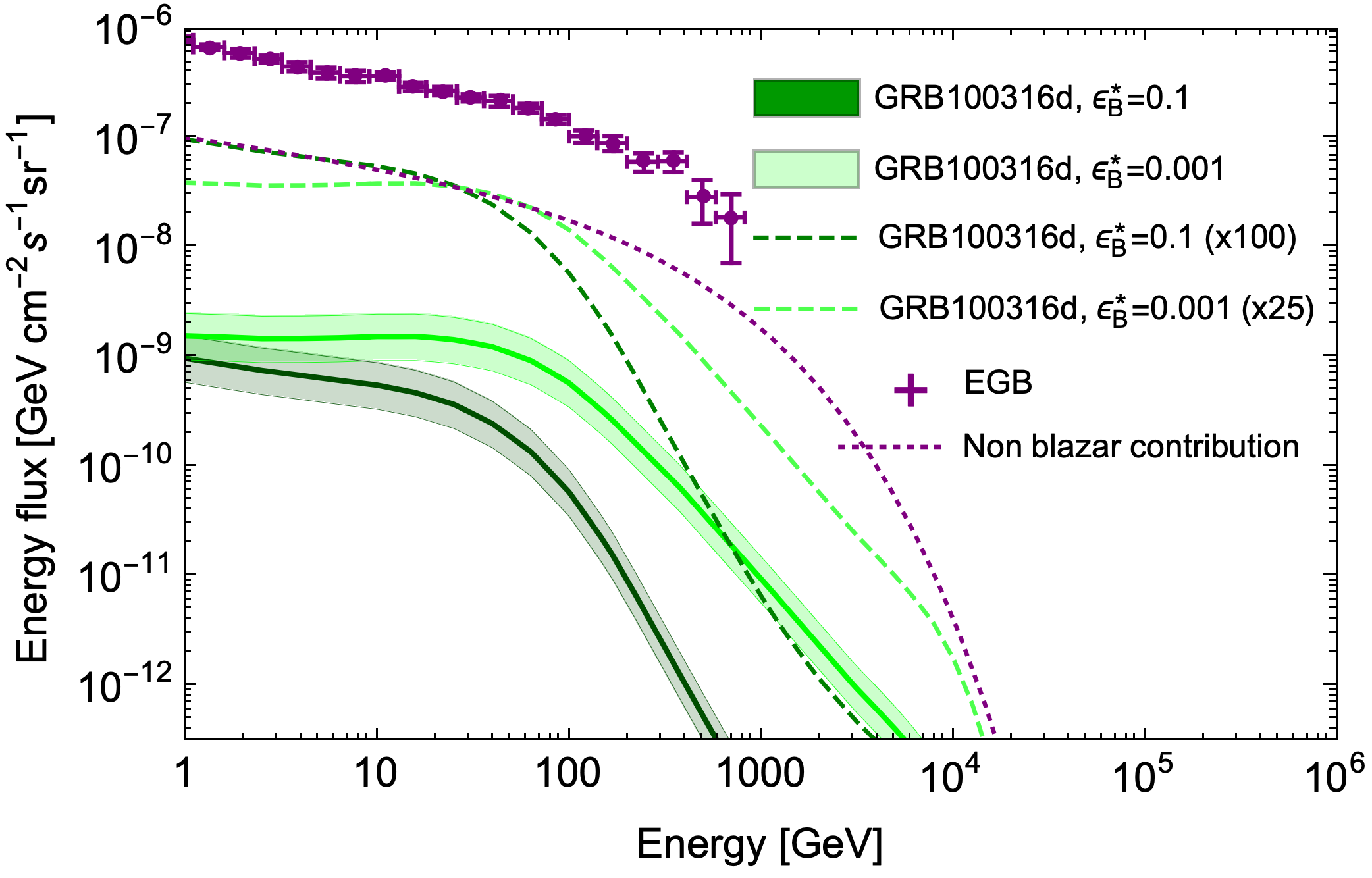
Let us now consider a population of ll-GRBs and assume that they describe UHECR and neutrino data as discussed in Boncioli et al. 2019. We also compute the contribution to the extragalactic diffuse gamma-ray background following Berezinsky & Kalashev 2016, and derive constraints for prompt emission duration and baryonic loading.
We here define the baryonic loading as , where quantifies the energy going into non-thermal baryons (). Using the results of our (leptonic) radiation modelling in Section 5 naturally implies that the energy dissipated in electrons is held constant. As energy conservation additionally dictates , a baryonic loading thus implies a increased wind luminosity (translating into an increased dissipated energy per collision ; In this case we need to redefine and to ensure that the leptonic radiation modelling yields the same results. As can be inferred from Eq. (9), the fraction of accelerated electrons would have to be adjusted accordingly. For the sake of simplicity we assume that all ll-GRBs are similar to one of our prototypes, although the typical duration may differ. Note, however, that there are already constraints on minute-scale long transients by IceCube (Aartsen et al. 2019b), which means that in this case the typical ll-GRB duration has to be probably longer than a few hundred seconds. The ll-GRBs with the prototype luminosities are assumed to be distributed over the Universe with a local rate (Sun et al. 2015), following the star formation rate of Kistler et al. 2009 with an additional evolution factor which has been proposed in Boncioli et al. 2019 to better fit UHECR data, see left panel of Fig. 10.
In order to describe UHECR and neutrino data, we can rescale11 1 The result in Boncioli et al. 2019 is degenerate in the product of these factors in Eq. (19); in that paper (e. g. Fig. 2) and were fixed, and a baryonic loading was found at the best-fit, consequently , which we have just rescaled here to the values used in this paper. from Boncioli et al. 2019 (almost independent of the collision radius)
| (19) |
The UHECR and neutrino description is degenerate in these parameters, which means that lower baryonic loadings could be compensated by longer durations.
An independent constraint can be obtained from the contribution to the extragalactic diffuse gamma-ray background. Due to the source evolution and the obtained HE gamma-ray emission, this contribution may be rather significant. We therefore show in Fig. 10, right panel, the expected contribution from a population of ll-GRBs given by prototype ul-GRB, and compare it with the EGB (Ackermann et al. 2015) measured by Fermi. Note that the EGB is expected to be driven by Active Galactic Nuclei, and the expected contribution from other source classes is small. We therefore show (dotted purple curve) the 14% of the EGB flux, since blazars already provide of contribution to the EGB, according to Ackermann et al. 2016. We thus identify this as the possible maximal contribution from ll-GRBs to the EGB. Comparing the curve GRB 100316D /ul-GRB (using which exhibits higher maximal energies, see left panel of Fig. 9) with the dotted curve, one easily finds the constraint22 2 We show in Fig. 10 the GRB contribution multiplied with the corresponding factor 100 as dark-green dashed cure, to illustrate that this enhancement factor saturates the possible non-blazar contribution to the EGB (it touches the dotted curve).
| (20) |
as the gamma-ray flux (for fixed luminosity) scales with these two quantities. We note that Eq. (20) may be used to break the degeneracy in Eq. (19), which yields the constraints
| (21) |
for the typical ll-GRB (and fixed), which is in fact consistent with the UHECR fit in Boncioli et al. 2019.
As a duration of s is a strong assumption for the typical ll-GRB duration, a related question is how large the baryonic loading can be in order to not to impact the observed SED (a high value of would allow reducing the required in Eq. (21)). We point out that the SED may be also produced by hadronic processes (including the second peak, such as from photons or large contributions by cascade emission), therefore this part can only give some rough estimates for the model discussed in this work. We focus on the pion production efficiency (the average fraction of energy lost into pion production), whereas protons in the source may produce other effects as well (such as proton synchrotron radiation). Additional effects would be expected from muon and pion synchrotron and radiation from secondary leptons produced e.g., via Bethe-Heitler.
Similar to Guetta et al. 2004, it can be analytically estimated as
| (22) |
(for small redshifts), taking the pitch angle-averaged inclusive cross section for production from Hummer et al. 2010. Here is a measure for the dynamical time-scale, i.e., the time the protons have to interact; it may be associated with the shell expansion time in our model. For ul-GRB, we have (for , , ), which leads to . From Boncioli et al. 2019 it is clear that (relatively high) pion production efficiencies are required if ll-GRBs are to power the diffuse neutrino flux. However, Hummer et al. 2012 have demonstrated that the actual value can be about an order of magnitude lower because this approximation neglects the energy dependence of the mean free path of the protons and the shape of the target photon spectrum (which are included in numerical calculations).
If the photons from the decays are fed into the electromagnetic cascade in the source, they will affect the SED at the highest energies. Since the injection luminosity into HE gamma-rays from these processes is and from Fig. 4 (the peak for HE gamma-rays is about a factor of ten lower than the one for gamma-rays), we have
| (23) |
in order not to affect the SED at all from these processes. For ul-GRB, we therefore find for this process to be on the safe side, where the lower number uses Eq. (22) at face value, and the upper value includes the estimate from Hummer et al. 2012.
We have verified with numerical simulations that for ul-GRB () the co-acceleration of protons (with the same injection index as electrons) with a baryonic loading of does not lead to additional, observable signatures or significantly change the observed spectrum. A more complete examination of this (including also e.g., the impact of a modified injection index of protons and/or the presence of heavier nuclei and an investigation of the maximal baryonic loading compatible with observed spectra) is clearly beyond the scope of this study.
As pointed out earlier, would require to lower the fraction of energy transferred to non-thermal electrons () and the fraction of accelerated electrons ( to ), which is closer to the non-exlcuded parameter space in Samuelsson et al. 2020. In this sense, the baryonic loading necessary to power the UHCER flux may require re-thinking some of the standard paradigms of the partition parameters within the GRB internal shock model.
7 Summary and conclusions
We have studied ll-GRBs as potential targets for multiwavelength astronomy and sources of UHECR nuclei. For this purpose we have selected three representative reference events out of the sample of detected ll-GRBs. The prototypes based on these reference events represent different types of ll-GRBs: sp-GRB is a single-peaked GRB of medium peak energy, low luminosity and low redshift, ul-GRB is an ultralong, multi-peaked GRB with low peak energy and hl-GRB is a single-peaked GRB with comparatively high luminosity and high redshift. Choosing the parameters of the outflow such that we reproduce the main features of the reference events, we self-consistently calculated the full spectral and temporal properties within the internal shock scenario and a leptonically-dominated radiation model.
We have found that ll-GRBs are indeed potential targets for multimessenger observations and could be detected by current/ future Imaging Air Cherenkov Telescopes (IACTs). This is mainly due to their low redshifts (and high local rate), which reduce the effect of EBL absorption at the highest energies. The intensity of the HE component is (for comparable intensity of the sub-MeV synchrotron peak) directly linked to the magnetic field strength . In our dynamical modelling of the outflow, varies throughout the evolution and is not set directly; Instead we control the fraction of energy supplying the magnetic field with the constant microphysics parameter . If we require a relatively high radiative efficiency (which implies lower bounds on ), we have found a significant VHE inverse Compton component if the magnetic field is powered by a fraction of order of the available internal energy. The intensity of the VHE emission increases systematically with decreasing . While this is expected in Thomson regime (recall that ), we observe the same tendency if the scatterings occur in Klein-Nishina regime. Therefore, a detailed numerical modelling over a broad energy range (including a VHE regime) may be used to constrain the physical conditions in the outflow and microphysics parameters, such as .
We have demonstrated that alternative probes of could be the (a) the optical flux (which increases with increasing ), (b) the low-energy photon spectral index (the low energy portion of the spectrum becomes steeper with increasing ) and (c) a delayed onset of the HE component (the early suppression of the VHE flux due to -absorption becomes larger with increasing ). We point out that those observables might not be reliable: For example, (a) the optical flux is subject to extinction in our own Galaxy and the host galaxy, which is in most cases not well constrained. On the other hand, (b) the photon index is largely impacted by the fit range of the observing instrument and the location of the spectral peak within the instrument range. Especially for ll-GRBs, which have generally low peak frequencies, this introduces uncertainties on measurement. Overall, it might be the joint analysis of all these observables that will make it possible to constrain the physical parameters of the sources and the processes at play, if a full numerical modelling is performed (including the dynamical evolution of parameters such as the magnetic field strength, volume and Lorentz factor).
Although using the same internal shock model commonly applied to GRB-HL, our simulations reside in a specific phase space of parameters such as dissipation radius, Lorentz factor and dissipated energy, due to the distinct properties of ll-GRBs (Daigne & Mochkovitch 2007). It is the combination of these parameters that result in specific properties of the observed spectra (like the intensity of the inverse Compton component). Thus, while some of the findings outlined above may also apply to high-luminosity events (see for example the discussion of in Daigne et al. 2011), our results can not easily be generalized to all GRBs.
We have also shown that ll-GRBs are able to accelerate nuclei to the UHE: Overall, the maximal energies of iron nuclei (protons) could be as high as GeV ( GeV). The highest maximal energies were achieved for large magnetic fields (set by large ), for which the inverse Compton efficiency was found to be low. This means that in our model, a ll-GRB can either accelerate UHECR to the highest energies or have high fluxes in the VHE regime. The high maximal energies in our model were possible by decoupling the production regions of the prompt -ray emission and the most energetic UHECR nuclei. The former is produced at intermediate radii, the latter in outer regions. The difference in radius is roughly an order of magnitude, questioning the validity of simplified one-zone models. However, outer collisions contribute less to the overall gamma-ray emission and more energy is dissipated at lower radii, for which the maximal cosmic-ray energies are lower. We point out that in order to calculate the true emitted spectra, additional assumptions on the injection spectrum and escape functions are required.
If ll-GRBs are to power the UHECR flux, a given local rate results in requirements for the typical energy emitted in UHECRs per GRB. This energy output is controlled by the product of burst duration and baryonic loading, which are thus degenerate. We have shown that the contribution to the diffuse gamma-ray background breaks this degeneracy and leads to an upper limit on the typical duration and a lower limit on the baryonic loading. An additional upper limit may come from hadronic signatures in the spectral energy distribution due to photo-pion production. Overall, we have estimated that basic consistency arises for a baryonic loading around 10-25. However, the energy partition parameters such as the fraction energy transferred to non-thermal electrons that correspond to this baryonic loading in combination with the results of our leptonic radiation modelling differ from the values discussed in the literature - a problem which is not specific to ll-GRBs, but applies to long GRBs as well if they are the dominant sources of UHECRs (see e.g., Heinze et al. 2020). Additionally, these results should be verified by including the hadronic and nuclear processes fully self-consistent in the spectral modelling.
We conclude that ll-GRBs are potential targets for multiwavelength and multimessenger astronomy. They are potentially within the sensitivity range of IACTs, and future instruments such as CTA and a multiwavelength coverage by optical/ UV surveys may help to constrain the physical processes at play in the source. ll-GRBs also fulfill the energetic requirements to accelerate cosmic-rays to UHE; To constrain the maximal baryonic loading in agreement with gamma-ray observations further studies with detailed radation modelling are required.
Acknowledgments
This work has been supported by the European Research Council (ERC) under the European Union’s Horizon 2020 research and innovation programme (Grant No. 646623). The work was supported by the International Helmholtz-Weizmann Research School for Multimessenger Astronomy, largely funded through the Initiative and Networking Fund of the Helmholtz Association. ŽB acknowledges the support of the Deutscher Akademischer Austauschdienst (DAAD) scholarship programme. This work was conducted in the context of the CTA Consortium. We use CTA instrument response functions, provided by the CTA Consortium and Observatory (version prod3b-v2). (See http://www.cta-observatory.org/science/cta-performance/.) We would also like to thank the CTA Consortium, for providing an initial review of the manuscript, as well as Anatoli Fedynitch and Filip Samuelsson for useful comments and discussion.
Data availability
Data available on request.
References
- Aartsen et al. (2014) Aartsen M. G., et al., 2014, arXiv e-prints
- Aartsen et al. (2015) Aartsen M. G., et al., 2015, Astrophys. J., 805, L5
- Aartsen et al. (2016) Aartsen M. G., et al., 2016, Astrophys. J., 824, 115
- Aartsen et al. (2017) Aartsen M. G., et al., 2017, Astrophys. J., 843, 112
- Aartsen et al. (2019a) Aartsen M. G., et al., 2019a, Phys. Rev. Lett., 122, 051102
- Aartsen et al. (2019b) Aartsen M. G., et al., 2019b, Phys. Rev. Lett., 122, 051102
- Abbasi et al. (2012) Abbasi R., et al., 2012, Nature, 484, 351
- Abdalla et al. (2017) Abdalla H., et al., 2017, Astron. Astrophys., 606, A59
- Abdalla et al. (2021) Abdalla H., et al., 2021, Science, 372, 1081
- Ackermann et al. (2015) Ackermann M., et al., 2015, Astrophys. J., 799, 86
- Ackermann et al. (2016) Ackermann M., et al., 2016, Phys. Rev. Lett., 116, 151105
- Aloy et al. (2018) Aloy M.-A., Cuesta-Martínez C. F., Obergaulinger M., 2018, Mon. Not. Roy. Astron. Soc., 478, 3576
- Amati (2006) Amati L., 2006, Mon. Not. Roy. Astron. Soc., 372, 233
- Amati et al. (2007) Amati L., Della Valle M., Frontera F., Malesani D., Guidorzi C., Montanari E., Pian E., 2007, Astron. Astrophys., 463, 913
- Asano & Inoue (2007) Asano K., Inoue S., 2007, Astrophys. J., 671, 645
- Asano & Mészáros (2011) Asano K., Mészáros P., 2011, ApJ, 739, 103
- Band et al. (1993) Band D., et al., 1993, Astrophys. J., 413, 281
- Bellm et al. (2018) Bellm E. C., et al., 2018, Publications of the Astronomical Society of the Pacific, 131, 018002
- Berezinsky & Kalashev (2016) Berezinsky V., Kalashev O., 2016, Phys. Rev., D94, 023007
- Biehl et al. (2018) Biehl D., Boncioli D., Fedynitch A., Winter W., 2018, Astron. Astrophys., 611, A101
- Boncioli et al. (2019) Boncioli D., Biehl D., Winter W., 2019, Astrophys. J., 872, 110
- Bosnjak et al. (2009) Bosnjak Z., Daigne F., Dubus G., 2009, Astron. Astrophys., 498, 677
- Bošnjak & Daigne (2014) Bošnjak v., Daigne F., 2014, Astron. Astrophys., 568, A45
- Bromberg et al. (2011) Bromberg O., Nakar E., Piran T., 2011, Astrophys. J. Lett., 739, L55
- Burrows et al. (2005) Burrows D. N., et al., 2005, Space Sci. Rev., 120, 165
- Bustamante et al. (2015) Bustamante M., Baerwald P., Murase K., Winter W., 2015, Nature Commun., 6, 6783
- Bustamante et al. (2017) Bustamante M., Murase K., Winter W., Heinze J., 2017, Astrophys. J., 837, 33
- Campana et al. (2006) Campana S., et al., 2006, Nature, 442, 1008
- Cano et al. (2017a) Cano Z., et al., 2017a, Astron. Astrophys., 605, A107
- Cano et al. (2017b) Cano Z., Wang S.-Q., Dai Z.-G., Wu X.-F., 2017b, Adv. Astron., 2017, 8929054
- Chand et al. (2020) Chand V., et al., 2020, ArXiv eprints
- Crumley et al. (2019) Crumley P., Caprioli D., Markoff S., Spitkovsky A., 2019, Mon. Not. Roy. Astron. Soc., 485, 5105
- Cummings et al. (2012) Cummings J. R., et al., 2012, GCN Circ. 13481
- D’Elia et al. (2018) D’Elia V., et al., 2018, Astron. Astrophys., 619, A66
- Daigne & Mochkovitch (1998) Daigne F., Mochkovitch R., 1998, Mon. Not. Roy. Astron. Soc., 296, 275
- Daigne & Mochkovitch (2000) Daigne F., Mochkovitch R., 2000, Astron. Astrophys., 358, 1157
- Daigne & Mochkovitch (2007) Daigne F., Mochkovitch R., 2007, Astron. Astrophys., 465, 1
- Daigne et al. (2011) Daigne F., Bosnjak Z., Dubus G., 2011, Astron. Astrophys., 526, A110
- Deil et al. (2018) Deil C., et al., 2018, PoS, ICRC2017, 766
- Dominguez et al. (2011) Dominguez A., et al., 2011, Mon. Not. Roy. Astron. Soc., 410, 2556
- Dong et al. (2010) Dong Y., Wu B., Li Y., Zhang Y., Zhang S., 2010, Science China Physics, Mechanics, and Astronomy, 53, 40
- Duran et al. (2012) Duran R., Bosnjak Z., Kumar P., 2012, Mon. Not. Roy. Astron. Soc., 424, 3192
- Fan et al. (2011) Fan Y.-Z., Zhang B.-B., Xu D., Liang E.-W., Zhang B., 2011, Astrophys. J., 726, 32
- Fioretti et al. (2021) Fioretti V., Ribeiro D., Humensky T. B., Bulgarelli A., Maier G., Moralejo A., Nigro C., 2021, PoS, ICRC2019, 673
- Foley et al. (2008) Foley S., McGlynn S., Hanlon L., McBreen S., McBreen B., 2008, A&A, 484, 143
- Fraija (2014) Fraija N., 2014, Mon. Not. Roy. Astron. Soc., 437, 2187
- Fraija et al. (2017) Fraija N., et al., 2017, Astrophys. J., 848, 15
- Fraija et al. (2021) Fraija N., Veres P., Beniamini P., Galvan-Gamez A., Metzger B. D., Duran R. B., Becerra R. L., 2021, Astrophys. J., 918, 12
- Frontera et al. (2000) Frontera F., et al., 2000, Astrophys. J. Suppl., 127, 59
- Gao et al. (2013) Gao S., Kashiyama K., Mészáros P., 2013, Astrophys. J. Lett., 772, L4
- Gao et al. (2017) Gao S., Pohl M., Winter W., 2017, Astrophys. J., 843, 109
- Ghirlanda et al. (2018) Ghirlanda G., et al., 2018, Astron. Astrophys., 609, A112
- Ghisellini et al. (2000) Ghisellini G., Celotti A., Lazzati D., 2000, Mon. Not. Roy. Astron. Soc., 313, 1
- Ghisellini et al. (2006) Ghisellini G., Ghirlanda G., Mereghetti S., Bosnjak Z., Tavecchio F., Firmani C., 2006, Mon. Not. Roy. Astron. Soc., 372, 1699
- Ghisellini et al. (2007) Ghisellini G., Ghirlanda G., Tavecchio F., 2007, Mon. Not. Roy. Astron. Soc., 382, 77
- Giannios (2010) Giannios D., 2010, Mon. Not. Roy. Astron. Soc., 408, 46
- Globus et al. (2015) Globus N., Allard D., Mochkovitch R., Parizot E., 2015, Mon. Not. Roy. Astron. Soc., 451, 751
- Godet et al. (2014) Godet O., et al., 2014, Proc. SPIE Int. Soc. Opt. Eng., 9144, 914424
- Granot et al. (1999) Granot J., Piran T., Sari R., 1999, Astrophys. J., 513, 679
- Gruber et al. (2014) Gruber D., et al., 2014, Astrophys. J. Suppl., 211, 12
- Guetta et al. (2004) Guetta D., Hooper D., Alvarez-Muniz J., Halzen F., Reuveni E., 2004, Astropart. Phys., 20, 429
- Hascoet et al. (2012) Hascoet R., Daigne F., Mochkovitch R., Vennin V., 2012, Mon. Not. Roy. Astron. Soc., 421, 525
- Heinze et al. (2019) Heinze J., Fedynitch A., Boncioli D., Winter W., 2019, Astrophys. J., 873, 88
- Heinze et al. (2020) Heinze J., Biehl D., Fedynitch A., Boncioli D., Rudolph A., Winter W., 2020, Mon. Not. Roy. Astron. Soc., 498, 5990
- Hummer et al. (2010) Hummer S., Ruger M., Spanier F., Winter W., 2010, Astrophys. J., 721, 630
- Hummer et al. (2012) Hummer S., Baerwald P., Winter W., 2012, Phys. Rev. Lett., 108, 231101
- Irwin & Chevalier (2016) Irwin C. M., Chevalier R. A., 2016, Mon. Not. Roy. Astron. Soc., 460, 1680
- Ivezić et al. (2019) Ivezić v., et al., 2019, Astrophys. J., 873, 111
- Kaneko et al. (2006) Kaneko Y., et al., 2006, Astrophys. J., 654, 385
- Kistler et al. (2009) Kistler M. D., Yuksel H., Beacom J. F., Hopkins A. M., Wyithe J. S. B., 2009, Astrophys. J., 705, L104
- Klose et al. (2019) Klose S., et al., 2019, Astron. Astrophys., 622, A138
- Knödlseder et al. (2016) Knödlseder J., et al., 2016, A&A, 593, A1
- Kobayashi et al. (1997) Kobayashi S., Piran T., Sari R., 1997, Astrophys. J., 490, 92
- Kovacevic et al. (2014) Kovacevic M., et al., 2014, Astron. Astrophys., 569, A108
- Kumar & Panaitescu (2003) Kumar P., Panaitescu A., 2003, MNRAS, 346, 905
- Kumar & Zhang (2014) Kumar P., Zhang B., 2014, Phys. Rept., 561, 1
- Lemoine & Pelletier (2010) Lemoine M., Pelletier G., 2010, Mon. Not. Roy. Astron. Soc., 402, 321
- Liang et al. (2007) Liang E., Zhang B., Dai Z. G., 2007, Astrophys. J., 662, 1111
- Lien et al. (2016) Lien A., et al., 2016, Astrophys. J., 829, 7
- Ligorini et al. (2021) Ligorini A., et al., 2021, Mon. Not. Roy. Astron. Soc., 502, 5065
- Liu et al. (2011) Liu R.-Y., Wang X.-Y., Dai Z.-G., 2011, Mon. Not. Roy. Astron. Soc., 418, 1382
- Liu et al. (2012) Liu X.-W., Wu X.-F., Lu T., 2012, AJ, 143, 115
- Mandal & Eichler (2010) Mandal S., Eichler D., 2010, Astrophys. J. L., 713, L55
- Marcowith et al. (2016) Marcowith A., et al., 2016, Rept. Prog. Phys., 79, 046901
- Marcowith et al. (2020) Marcowith A., Ferrand G., Grech M., Meliani Z., Plotnikov I., Walder R., 2020, Liv. Rev. Comput. Astrophys., 6, 1
- Meegan et al. (2009) Meegan C., et al., 2009, Astrophys. J., 702, 791
- Murase & Ioka (2013) Murase K., Ioka K., 2013, Phys. Rev. Lett., 111, 121102
- Murase et al. (2006) Murase K., Ioka K., Nagataki S., Nakamura T., 2006, Astrophys. J., 651, L5
- Murase et al. (2008) Murase K., Ioka K., Nagataki S., Nakamura T., 2008, Phys.Rev., D78, 023005
- Nakar (2015) Nakar E., 2015, Astrophys. J., 807, 172
- Nakar & Sari (2012) Nakar E., Sari R., 2012, ApJ, 747, 88
- Nakar et al. (2009) Nakar E., Ando S., Sari R., 2009, Astrophys. J., 703, 675
- Nigro et al. (2019) Nigro C., et al., 2019, Astron. Astrophys., 625, A10
- Oganesyan et al. (2017) Oganesyan G., Nava L., Ghirlanda G., Celotti A., 2017, ApJ, 846, 137
- Oganesyan et al. (2019) Oganesyan G., Nava L., Ghirlanda G., Melandri A., Celotti A., 2019, Astron. Astrophys., 628, A59
- Perinati et al. (2012) Perinati E., Tenzer C., Santangelo A., Cordier B., Gotz D., Fraser G. W., Osborne J. P., 2012, in Takahashi T., Murray S. S., den Herder J.-W. A., eds, Society of Photo-Optical Instrumentation Engineers (SPIE) Conference Series Vol. 8443, Space Telescopes and Instrumentation 2012: Ultraviolet to Gamma Ray. p. 84434T, doi:10.1117/12.925458
- Pescalli et al. (2015) Pescalli A., Ghirlanda G., Salafia O. S., Ghisellini G., Nappo F., Salvaterra R., 2015, Mon. Not. Roy. Astron. Soc., 447, 1911
- Pian et al. (2000) Pian E., et al., 2000, Astrophys. J., 536, 778
- Plotnikov et al. (2013) Plotnikov I., Pelletier G., Lemoine M., 2013, Mon. Not. Roy. Astron. Soc., 430, 1280
- Poolakkil et al. (2021) Poolakkil S., et al., 2021, arXiv e-prints, p. arXiv:2103.13528
- Preece et al. (2002) Preece R. D., Briggs M. S., Giblin T. W., Mallozzi R. S., Pendleton G. N., Paciesas W. S., Band D. L., 2002, The Astrophysical Journal, 581, 1248
- Rees & Meszaros (1994) Rees M. J., Meszaros P., 1994, ApJ, 430, L93
- Reville & Bell (2014) Reville B., Bell A. R., 2014, Mon. Not. Roy. Astron. Soc., 439, 2050
- Rudolph et al. (2020) Rudolph A., Heinze J., Fedynitch A., Winter W., 2020, Astrophys. J., 893, 72
- Sagiv et al. (2014) Sagiv I., et al., 2014, Astron. J., 147, 79
- Samuelsson et al. (2019) Samuelsson F., Bégué D., Ryde F., Pe’er A., 2019, Astrophys. J., 876, 93
- Samuelsson et al. (2020) Samuelsson F., Bégué D., Ryde F., Pe’er A., Murase K., 2020, arXiv e-prints, p. arXiv:2005.02417
- Sari et al. (1998) Sari R., Piran T., Narayan R., 1998, Astrophys. J. Lett., 497, L17
- Schulze et al. (2014) Schulze S., et al., 2014, Astron. Astrophys., 566, A102
- Senno et al. (2016) Senno N., Murase K., Meszaros P., 2016, Phys. Rev., D93, 083003
- Siellez & LIGO Team (2018) Siellez K., LIGO Team 2018, in American Astronomical Society Meeting Abstracts #231. p. 107.06
- Singer et al. (2013) Singer L. P., et al., 2013, Astrophys. J., 776, L34
- Sironi & Spitkovsky (2009) Sironi L., Spitkovsky A., 2009, Astrophys. J., 698, 1523
- Sironi et al. (2013) Sironi L., Spitkovsky A., Arons J., 2013, ApJ, 771, 54
- Sparre & Starling (2012) Sparre M., Starling R. L. C., 2012, MNRAS, 427, 2965
- Starling et al. (2011) Starling R. L. C., et al., 2011, Mon. Not. Roy. Astron. Soc., 411, 2792
- Suda et al. (2021) Suda Y., et al., 2021, PoS, ICRC2021, 797
- Sun et al. (2015) Sun H., Zhang B., Li Z., 2015, Astrophys. J., 812, 33
- Virgili et al. (2009) Virgili F., Liang E., Zhang B., 2009, Mon. Not. Roy. Astron. Soc., 392, 91
- Volnova et al. (2017) Volnova A. A., et al., 2017, Mon. Not. Roy. Astron. Soc., 467, 3500
- Waxman et al. (2007) Waxman E., Meszaros P., Campana S., 2007, Astrophys. J., 667, 351
- Wu et al. (2011) Wu C., Qiu Y. L., Cai H. B., 2011, Proceedings of the International Astronomical Union, 7, 421–422
- Zhang et al. (2012) Zhang B.-B., Fan Y.-Z., Shen R.-F., Xu D., Zhang F.-W., Wei D.-M., Burrows D. N., Zhang B., 2012, Astrophys. J., 756, 190
- Zhang et al. (2018) Zhang B. T., Murase K., Kimura S. S., Horiuchi S., Mészáros P., 2018, Phys. Rev., D97, 083010
- Zhang et al. (2021) Zhang B. T., Murase K., Veres P., Mészáros P., 2021, Astrophys. J., 920, 55
Appendix A Theoretical predictions for the photon spectrum
We describe the theoretical predictions of a spectrum produced by an electron distribution following a power law of index above a minimum Lorentz factor . This is used in the following, as part of the interpretation of the simulated spectra and light curves. We pay special attention to the processes that can shape the spectrum below the synchrotron peak and to the dependence of a potential HE signal on the GRB parameters.
For the following it is helpful to define
| (24) |
which represents the Lorentz factor of electrons whose synchrotron cooling time-scale is equal to the shell expansion time-scale .
We want to summarize basic theoretical predictions on the shape of the SED. These are generally applicable to GRBs, and not specific to ll-GRBs. However, due to the specific properties of ll-GRBs compared to high-luminosity events (lower wind luminosities, lower Lorentz factors), different regimes may be realized. In the following we will discuss the differential spectrum (usually represented as , where is the number of photons at a given energy ) and the spectral index of the differential photon flux (), assuming a power-law spectral shape. We will denote the slope below the peak of as , as described e.g., by the Band function (Band et al. 1993). We follow Sari et al. 1998 and recapitulate the shape of the pure synchrotron spectrum , although omitting the effect of synchrotron self-absorption. Generally, the spectral shape can be divided in two regimes:
- (a)
Fast-cooling regime : :
(25) Here is the synchrotron frequency of an electron with Lorentz factor , the synchrotron frequency of an electron with Lorentz factor .
All (initial) electrons cool via synchrotron cooling on the dynamical time-scale and thus convert their energy relatively efficiently into radiation. The spectral index of the photon flux below the peak of (located at ) is given by .
- (b)
Slow-cooling regime : :
(26) Not all electrons cool via synchrotron cooling on the dynamical time-scale, some thus don’t convert their energy efficiently into radiation. The spectral index of the photon flux below the peak of is given by .
With pure synchrotron radiation, one achieves spectral indeces below the peak that are either equal to or , which is not in agreement with observations (e.g., Preece et al. 2002; Ghisellini et al. 2000, see also current GRB catalog spectral analysis as in e.g. Poolakkil et al. 2021; Gruber et al. 2014; Lien et al. 2016). For the slow-cooling regime one additionally suffers from a poor radiative efficiency (defined as , the integrated (final) photon energy divided by the integral injected electron energy). This further reduces the already small overall efficiency of the internal shock model, imposing an even higher engine power. Note that Daigne et al. 2011 also identified the marginally fast cooling regime, for which and low-energy spectral slopes of can be realized while still achieving a relatively high radiative efficiency. Recently Oganesyan et al. 2017 fitted the sample of prompt GRB spectra observed down to 0.5 keV energies by the two low energy power-laws and a break energy corresponding to the cooling break frequency; they found a small ratio of the spectral peak energy and the cooling break frequency, suggesting a regime of moderately fast cooling. This scenario has also been explored in Oganesyan et al. 2019, with a focus on optical fluxes.
Additional effects can shape the spectra and impact :
- 1.
Synchrotron self-absorption: At the lowest energies, electrons can re-absorb photons through synchrotron self-absorption. This gives rise to an additional break in the photon spectrum.
- 2.
Inverse Compton radiation: introduces a second peak at high energies. The spectral shape below spectral peak may be affected by inverse Compton scatterings, resulting in harder low energy spectral slopes (Nakar et al. 2009; Daigne et al. 2011; Duran et al. 2012).
- 3.
-absorption: If the photon densities are high, pairs annihilate to lepton pairs at the highest energies. Those pairs are expected to contribute via synchrotron radiation at low energies (and therefore may reshape the spectrum below the synchrotron peak) and inverse Compton radiation (at intermediate energies) (Asano & Inoue 2007; Asano & Mészáros 2011). As densities scale inversely with the comoving volume, this is especially relevant for collisions at low radii and/or with low Lorentz factors.
If those theoretical predictions are compared to data/ results of spectral fits, one has to be aware that the reported slopes are usually determined by fitting either a Band empirical function or a cut-off power law, and that resulting slopes are very sensitive to the functional fitting range which is informed by the sensitivity of the experiments.
Appendix B Parameter space exploration for different values of


In this section we show how during the jet evolution the different emission regimes are achieved (with different respective properties of the observed radiation, defined by analytical estimates), depending largely on for the three model GRBs. For a detailed discussion on the theoretical predictions of the corresponding photon spectra see Section A. For this purpose, we examine different choices of (-axis of Fig. 11) and different collisions between single layers in the GRB evolution, assuming the same fireball evolution which is set by and Lorentz factor distribution for each GRB. The individual collisions are numbered chronologically by the time they occur in the source frame (-axis of Fig. 11). For each collision and we evaluate the following two conditions:
- 1.
Fast cooling regime
This regime is realized if is satisfied. In this case, all electrons cool on the dynamical time-scale, which translates into a relatively high radiative efficiency.The region in the parameter space fulfilling this criterium are marked blue in Fig. 11.
- 2.
Inverse Compton scatterings occuring in the Klein-Nishina regime
Following Daigne et al. 2011 and Nakar et al. 2009, we define this regime as the region where . Here we calculate the Compton parameter directly from the microphysics parameters as , and . The region in the parameter space where this criterium is satisfied are marked purple in Fig. 11.
If both criteria are met, the resulting overlap is a dark purple region. Due to the low luminosity of the GRBs, relatively high values of are required for the fast cooling regime condition– especially for ul-GRB, where even for this condition is not satisfied in all collisions. The Klein-Nishina inverse Compton regime is generally realized for lower values of .
Appendix C Impact of the different radiative processes
Since the impact of secondary lepton pairs created by pair annihilation was not accounted for in past studies, e.g. Bosnjak et al. 2009, we explicitly study this effect in the following section. Given that some recent studies (Oganesyan et al. 2019; Samuelsson et al. 2020) compare the observed spectra to synchrotron predicitons, we also show the obtained spectra for a pure synchrotron calculation.


The lower panel shows the photon index of , the dashed lines correspond to the synchrotron predictions (, and ) , the solid line marks the position of maxima/minima of
In Fig. 12 we show the time-integrated spectra for sp-GRB, ul-GRB and hl-GRB for . Comparing to a full radiative treatment of all processes, we show the spectra obtained without taking into account secondary electrons produced by -annihilation, as well as the pure synchrotron prediction. We first examine the impact of secondaries created by -pair production. Due to their synchrotron radiation, they enhance the flux in the eV-regime by roughly one order of magnitude – stressing the importance of a full radiative treatment when comparing predictions to observations in the optical regime. At intermediate energies around - keV, the inverse Compton scatterings of the -produced pairs result in a slight enhancement of the flux. As the intensity absorption depends on the level of VHE emission, these additional effects will be more pronounced for a strong inverse Compton component (and thus, low ).
The pure synchrotron case has a cutoff in the observed spectra at approximately keV. In the optical regime, the prediction is equal to the case without impact of secondaries from -pair production. Even in the case of moderate magnetic fields (as in this example), the effects of inverse Compton radiation should thus be taken into account when modelling the spectra.
Appendix D Time-resolved spectra


We investigate the observed temporal evolution of single pulses by analyzing GRB SP. The time-resolved spectra for this prototype are shown in Fig. 13 for (upper panel) and (lower panel). The spectra are integrated on time scale of 0.5 s. We again point out that the overall fireball efficiency for is very low and it thus might not be a realistic choice of parameter. However, it shows the most pronounced effects of inverse Compton scatterings, which is why we will study it here. Single pulses in SP-UL and the the single pulse of hl-GRB in principle show the similar behaviour.
For both cases the evolution of the peak energy shows a trend generally observed during the prompt GRB emission (e.g. Kaneko et al. 2006): The spectrum evolves from harder to softer one with time.
For the spectral index we also predict an evolution with time. Observed values of should be considered cautiously, keeping in mind the instrumental energy range used for spectral fit, burst brightness, and the time scale used for spectral integration, which affect the results.
For low values of , the synchrotron cooling time is comparable to the inverse Compton cooling time even at early times. This enables efficient inverse Compton scatterings at early times, even despite high -absorption. As an effect, the HE component is clearly visible at early times for , but not for .
Appendix E Energy loss rates for different processes
For a better understanding of the physical processes in the source we studied the energy loss rates for both leptons and hadrons.
E.1 Leptonic loss rates
Fig. 14 contains the energy loss rates for different leptonic processes at the maximum of the pulse (where most of the energy is disspated) for and for sp-GRB. Synchrotron losses dominate over the entire range of injection even for (for most collisions the fast cooling regime condition is satisfied). Adiabatic cooling due to the shell expansion is sub-dominant compared to both inverse Compton and synchrotron cooling. For lower electron energies and low magnetic fields (), inverse Compton coolings may dominate over both adiabatic and synchrotron cooling.


E.2 Hadronic loss rates
As an addition to Section 6, we show the energy loss rates for iron and protons for both, an early (close to the source) and a late (far out) collision for sp-GRB (). The early collision is chosen such that is minimal, the late collision corresponds to the maximum of . Note that while acceleration and synchrotron losses depend on the magnetic field, we expect the hadronic processes to be almost independent of the magnetic field (given that the target photon fields are quite similar, which they are by construction around the peak). We notice that for collisions which have small maximal cosmic-ray energies, photo-hadronic losses play an important role, while the maximal cosmic-ray energy (for iron) is achieved in a case where the energy is limited by adiabatic cooling. At this relatively late collision at lage radius the photon densities are low (as the volume scales with ).

