ANCER: Anisotropic Certification via Sample-wise Volume Maximization
Abstract
Randomized smoothing has recently emerged as an effective tool that enables certification of deep neural network classifiers at scale. All prior art on randomized smoothing has focused on isotropic certification, which has the advantage of yielding certificates that can be easily compared among isotropic methods via -norm radius. However, isotropic certification limits the region that can be certified around an input to worst-case adversaries, i.e. it cannot reason about other “close”, potentially large, constant prediction safe regions. To alleviate this issue, (i) we theoretically extend the isotropic randomized smoothing and certificates to their generalized anisotropic counterparts following a simplified analysis. Moreover, (ii) we propose evaluation metrics allowing for the comparison of general certificates – a certificate is superior to another if it certifies a superset region – with the quantification of each certificate through the volume of the certified region. We introduce AnCer, a framework for obtaining anisotropic certificates for a given test set sample via volume maximization. We achieve it by generalizing memory-based certification of data-dependent classifiers. Our empirical results demonstrate that AnCer achieves state-of-the-art and certified accuracy on CIFAR-10 and ImageNet in the data-dependence setting, while certifying larger regions in terms of volume, highlighting the benefits of moving away from isotropic analysis. Our code is available in this repository.
1 Introduction
The well-studied fact that Deep Neural Networks (DNNs) are vulnerable to additive imperceptible noise perturbations has led to a growing interest in developing robust classifiers (Goodfellow et al. 2015; Szegedy et al. 2014). A recent promising approach to achieve state-of-the-art provable robustness (i.e. a theoretical bound on the output around every input) at the scale of ImageNet (Deng et al. 2009) is randomized smoothing (Lecuyer et al. 2019; Cohen et al. 2019). Given an input and a network , randomized smoothing constructs such that , where the certification region is characterized by , , and the smoothing distribution . For instance, Cohen et al. 2019 showed that if , then is an -ball whose radius is determined by , and . Since then, there has been significant progress towards the design of leading to the largest for all inputs . The interplay between characterized by , and -balls, and a notion of optimal distribution has been previously studied (Yang et al. 2020).
Despite this progress, current randomized smoothing approaches provide certification regions that are isotropic in nature, limiting their capacity to certifying smaller and worst-case regions. We provide an intuitive example of this behavior in Figure 1. The isotropic nature of in prior art is due to the common assumption that the smoothing distribution is identically distributed (Yang et al. 2020; Kumar et al. 2020; Levine & Feizi 2021). Moreover, comparisons between various randomized smoothing approaches were limited to methods that produce the same certificate, with no clear metrics for comparing with other certificates. In this paper, we address both concerns and present new state-of-the-art certified accuracy results on both CIFAR-10 and ImageNet datasets.


Our contributions are threefold. (i) We provide a general and simpler analysis compared to prior art (Cohen et al. 2019; Yang et al. 2020) that paves the way for the certification of anisotropic regions characterized by any norm, holding prior art as special cases. We then specialize our result to regions that, for a positive definite , are ellipsoids, i.e. , and generalized cross-polytopes, i.e. , generalizing both (Cohen et al. 2019) and (Lecuyer et al. 2019; Yang et al. 2020) certification (Section 4). (ii) We introduce a new evaluation framework to compare methods that certify general (isotropic or anisotropic) regions. We compare two general certificates by defining that a method certifying is superior to another certifying , if is a strict superset to . Further, we define a standalone quantitative metric as the volume of the certified region, and specialize it for the cases of ellipsoids and generalized cross-polytopes (Section 5). (iii) We propose AnCer, an anisotropic certification method that performs sample-wise (i.e. per sample in the test set) region volume maximization (Section 6), generalizing the data-dependent, memory-based solution from Alfarra et al. 2022. Through experiments on CIFAR-10 (Krizhevsky 2009) and ImageNet (Deng et al. 2009), we show that restricting AnCer’s certification region to and -balls outperforms state-of-the-art and results from previous works (Yang et al. 2020; Alfarra et al. 2022). Further, we show that the volume of the certified regions are significantly larger than all existing methods, thus setting a new state-of-the-art in certified accuracy. We highlight that while we effectively achieve state-of-the-art performance, it comes at a high cost given the data-dependency requirements. A discussion of the limitations of the solution is presented in Section 6.
Notation.
We consider a base classifier , where is a probability simplex over classes, i.e. and , for . Further, we use to be a sample input and its corresponding true label drawn from a test set , and to be the output of at the correct class. We use to be the typically defined norm (), and or for to be a composite norm defined with respect to a positive definite matrix as .
2 Related Work
Verified Defenses.
Since the discovery that DNNs are vulnerable against input perturbations (Goodfellow et al. 2015; Szegedy et al. 2014), a range of methods have been proposed to build classifiers that are verifiably robust (Huang et al. 2017; Gowal et al. 2019; Bunel et al. 2018; Salman et al. 2019b). Despite this progress, these methods do not yet scale to the networks the community is interested in certifying (Tjeng et al. 2019; Weng et al. 2018).
Randomized Smoothing.
The first works on randomized smoothing used Laplacian (Lecuyer et al. 2019; Li et al. 2019) and Gaussian Cohen et al. 2019 distributions to obtain and -ball certificates, respectively. Several subsequent works improved the performance of smooth classifiers by training the base classifier using adversarial augmentation (Salman et al. 2019a), regularization (Zhai et al. 2019), or general adjustments to training routines (Jeong & Shin 2020). Recent work derived -norm certificates for other isotropic smoothing distributions (Yang et al. 2020; Levine & Feizi 2020; Zhang et al. 2019). Concurrently, Dvijotham et al. 2020 developed a framework to handle arbitrary smoothing measures in any -norm; however, the certification process requires significant hyperparameter tuning. Similarly, Mohapatra et al. 2020 introduces larger certificates that require higher-order information, yet do not provide a closed-form solution. This was followed by a complementary data-dependent smoothing approach, where the parameters of the smoothing distribution were optimized per test set sample to maximize the certified radius at an individual input (Alfarra et al. 2022). All prior works considered smoothing with isotropic distributions and hence certified isotropic -ball regions. In this paper, we extend randomized smoothing to certify anisotropic regions, by pairing it with a generalization of the data-dependent framework (Alfarra et al. 2022) to maximize the certified region at each input point.
3 Motivating Anisotropic Certificates
Certification approaches aim to find the safe region , where . Recent randomized smoothing techniques perform this certification by explicitly optimizing the isotropic certified region around each input (Alfarra et al. 2022), obtaining state-of-the-art performance as a result. Despite this optimality, we note that any -norm certificate is worst-case from the perspective of that norm, as it avoids adversary regions by limiting its certificate to the -closest adversary. This means that it can only enjoy a radius that is at most equal to the distance to the closest decision boundary. However, decision boundaries of general classifiers are complex, non-linear, and non-radially distributed with respect to a generic input sample (Karimi et al. 2019). This is evidenced by the fact that, within a reasonably small -ball around an input, there are often only a small set of adversary directions (Tramèr et al. 2017; Tramèr et al. 2018) (e.g. see the decision boundaries in Figure 1). As such, while -norm certificates are useful to reason about worst-case performance and are simple to obtain given previous works (Cohen et al. 2019; Yang et al. 2020; Lee et al. 2019), they are otherwise uninformative in terms of the shape of decision boundaries, i.e. which regions around the input are safe.
To visualize these concepts, we illustrate the decision boundaries of a base classifier trained on a toy 2-dimensional, radially separable (with respect to the origin) binary classification dataset, and consider two different input test samples (see Figure 1). We compare the optimal isotropic and anisotropic certified regions of different shapes at these points. In Figures 1(a) and 1(b), we compare an isotropic cross-polytope (of the form ) with an anisotropic generalized cross-polytope (of the form ), while in Figures 1(c) and 1(d) we compare an isotropic ball (of the form ) with an anisotropic ellipsoid (of the form ). Notice that in Figures 1(a) and 1(c), due to the curvature of the classification boundary (shown in white), the optimal certification region is isotropic in nature, which is evidenced by the similarities of the optimal isotropic and anisotropic certificates. On the other hand, in Figures 1(b) and 1(d), the location of the decision boundary allows for the anisotropic certified regions to be considerably larger than their isotropic counterparts, as they are not as constrained by the closest decision boundary, i.e. the worst-case performance. We note that these differences are further highlighted in higher dimensions, and we study them for a single CIFAR-10 test set sample in Appendix A.1.


As shown, anisotropic certification reasons more closely about the shape of the decision boundaries, allowing for further insights into constant prediction (safe) directions. In Figure 2, we present a series of test set images , as well as practically indistinguishable images which are not inside the optimal certified isotropic -balls for each input sample, yet are within the anisotropic certified regions. This showcases the merits of using anisotropic certification for characterizing larger safe regions.
4 Anisotropic Certification
One of the main obstacles in enabling anisotropic certification is the complexity of the analysis required. To alleviate this, we follow a Lipschitz argument first observed by Salman et al. 2019a and Jordan & Dimakis 2020 and propose a simple and general certification analysis. We start with the following two observations. All proofs are in Appendix B.
Proposition 1.
Consider a differentiable function . If where has a dual norm , then is -Lipschitz under norm , that is .
Given the previous proposition, we formalize certification as follows:
Theorem 1.
Let , be -Lipschitz continuous under norm , and . Then, we have for all satisfying:
Theorem 1 provides an norm robustness certificate for any -Lipschitz classifier under . The certificate is only informative when one can attain a tight non-trivial estimate of , ideally , which is generally difficult when is an arbitrary neural network.
Framework Recipe. In light of Theorem 1, randomized smoothing can be viewed differently as an instance of Theorem 1 with the favorable property that the constructed smooth classifier enjoys an analytical form for by design. As such, to obtain an informative certificate, one must, for an arbitrary choice of a smoothing distribution, compute the analytic Lipschitz constant under for . While there can exist a notion of “optimal” smoothing distribution for a given choice of certificate, as in part addressed earlier for the isotropic , and certificates (Yang et al. 2020), this is not the focus of this paper. The choice of the smoothing distribution in later sections is inspired by previous work for the purpose of granting anisotropic certificates. This recipe complements randomized smoothing works based on Neyman-Pearson’s lemma (Cohen et al. 2019) or the Level-Set and Differential Method (Yang et al. 2020).
We will deploy this framework recipe to show two specializations for anisotropic certification, namely ellipsoids (Section 4.1) and generalized cross-polytopes (Section 4.2).11 1 Our analysis also grants a certificate for a mixture of Gaussians smoothing distribution (see Appendix B.1)..
4.1 Certifying Ellipsoids
In this section, we consider the certification under norm, or , that has a dual norm . Note that both and define an ellipsoid. Despite that the following results hold for any positive definite , we assume for efficiency reasons that is diagonal throughout. First, we consider the anisotropic Gaussian smoothing distribution with the smooth classifier defined as . Considering the classifier , where is the standard Gaussian CDF, and following Theorem 1 to grant an certificate for , we derive the Lipschitz constant under , in the following proposition.
Proposition 2.
is -Lipschitz (i.e. ) under the norm.
Corollary 1.
Let , then for all satisfying:
Corollary 1 holds the certification from Zhai et al. 2019 as a special case for when .22 2 A similar result was derived in the appendix of Fischer et al. 2020; Li et al. 2020 with a more involved analysis by extending Neyman-Pearson’s lemma.
4.2 Certifying Generalized Cross-Polytopes
Here we consider certification under the norm defining a generalized cross-polytope, i.e. the set , as opposed to the -bounded set that defines a cross-polytope, i.e. . As with the ellipsoid case and despite that the following results hold for any positive definite , for the sake of efficiency, we assume to be diagonal throughout. For generalized cross-polytope certification, we consider an anisotropic Uniform smoothing distribution , which defines the smooth classifier . Following Theorem 1 and to certify under the norm, we compute the Lipschitz constant of under the norm, which is the dual norm of (see Appendix B), in the next proposition.
Proposition 3.
The classifier is -Lipschitz (i.e. ) under the norm.
Corollary 2.
Let , then for all satisfying:
Corollary 2 holds the certification from Yang et al. 2020 as a special case for when .
5 Evaluating Anisotropic Certificates
With the anisotropic certification framework presented in the previous section, the question arises: “Given two general (isotropic or anisotropic) certification regions and , how can one effectively compare them?”. We propose the following definition to address this issue.
Definition 1.
For a given input point , consider the two certification regions and obtained for two classifiers and , i.e. and where . We say is a "superior certificate" to (i.e. ), if and only if, .
This definition is a natural extension from the radius-based comparison of -ball certificates, providing a basis for evaluating anisotropic certification. To compare an anisotropic to an isotropic region of certification, it is not immediately clear how to (i) check that an anisotropic region is a superset to the isotropic region, and (ii) if it were a superset, how to quantify the improvement of the anisotropic region over the isotropic counterpart. In Sections 5.1 and 5.2, we tackle these issues for the particular cases of ellipsoid and generalized cross-polytope certificates.
5.1 Evaluating Ellipsoid Certificates
Comparing Balls to Ellipsoids (Specialization of Definition 1).
Recall that if , our ellipsoid certification in Corollary 1 recovers as a special case the isotropic -ball certification of Cohen et al. 2019; Salman et al. 2019a; Zhai et al. 2019. Consider the certified regions and for given . Since we take , the maximum enclosed -ball for the ellipsoid is given by the set , and thus . Therefore, it suffices that (i.e. ), to say that is a superior certificate to the isotropic as per Definition 1.
Quantifying Certificates.
The aforementioned specialization is only concerned with whether our ellipsoid certified region is “superior” to the isotropic -ball without quantifying it. A natural solution is to directly compare the volumes of the certified regions. Since the volume of an ellipsoid given by is (Kendall 2004), we directly compare the proxy radius defined for as , since larger correspond to certified regions with larger volumes. Note that , which is the root of the volume up to a constant factor, can be seen as a generalization to the certified radius in the case when .
5.2 Evaluating Generalized Cross-Polytope Certificates
Comparing Balls to Generalized Cross-Polytopes (Specialization of Definition 1).
Consider the certificates , , and , where we take . Note that since , then as per Definition 1, it suffices that (i.e. ) to say that the anisotropic generalized cross-polytope is superior to the isotropic -ball .
Quantifying Certificates.
Following the approach proposed in the case, we quantitatively compare the generalized cross-polytope certification of Corollary 2 to the certificate through the volumes of the two regions. We first present the volume of the generalized cross-polytope.
Proposition 4.
.
Following this definition, we define the proxy radius for in this case to be . As with the case, larger correspond certified regions with larger volumes. As in the ellipsoid case, can be seen as a generalization to the certified radius when .
6 AnCer: Sample-wise Volume Maximization for Anisotropic Certification
Given the results from the previous sections, we are now equipped to certify anisotropic regions, in particular ellipsoids and generalized cross-polytopes. As mentioned in Section 4, these regions are generally defined as for a given parameter of the smoothing distribution , an -norm (), and a gap value of . At this point, one could simply take an anisotropic distribution with arbitrarily chosen parameters and certify a trained network at any input point , in the style of what was done in the previous randomized smoothing literature with isotropic distributions. However, the choice of is more complex in the anisotropic case. A fixed choice of anisotropic could severely underperform the isotropic case – take, for example, the anisotropic distribution of Figure 1(d) applied to the input of Figure 1(c).
Instead of taking a fixed , we generalize the framework introduced by Alfarra et al. 2022, where parameters of the smoothing distribution are optimized per input test point (i.e. in a sample-wise fashion) so as to maximize the resulting certificate. The goal of the optimization in (Alfarra et al. 2022) is, at a point , to maximize the isotropic region described in Section 4.1 (i.e. ), where is the gap and a function of and . In the isotropic case, this generalizes to maximizing the region , which can be achieved by maximizing radius through , obtaining (Alfarra et al. 2022).
For the general anisotropic case, we propose AnCer, whose objective is to maximize the volume of the certified region through the proxy radius, while satisfying the superset condition with respect to the maximum isotropic radius, . In the case of the ellipsoids and generalized cross-polytopes as presented in Sections 5.1 and 5.2, respectively, AnCer’s optimization problem can be written as:
| (1) |
where is the gap value under the anisotropic smoothing distribution. That is,
for and , respectively. This is a nonlinear constrained optimization problem that is challenging to solve. As such, we relax it, and solve instead:
given a hyperparameter . While the constraint is not explicitly required to enforce the superset condition over the isotropic case, it proved itself beneficial from an empirical perspective. To sample from the distribution parameterized by (in our case, either a Gaussian or Uniform), we make use of the reparameterization trick, as in Alfarra et al. 2022. The solution of this optimization problem can be found iteratively by performing projected gradient ascent, as detailed in Algorithm 1. A standalone implementation for the AnCer optimization stage is presented in Listing in Appendix C.
Memory-based Anisotropic Certification. While each of the classifiers induced by the parameter , i.e. , is robust by definition as presented in Section 4, the certification of the overall data-dependent classifier is not necessarily sound due to the optimization procedure for each . This is a known issue in certifying data-dependent classifiers, and is addressed by Alfarra et al. 2022 through the use of a memory-based procedure. In Appendix D, we present an adapted version of this algorithm to AnCer. All subsequent results are obtained following this procedure.
Limitations of AnCer. Given AnCer uses a memorization procedure similar to the one presented in Alfarra et al. 2022, it incurs limitations on memory and runtime complexity. Note that in memory-based data-dependent certification there is a single procedure for both certification and inference in contrast with the fixed setting from Cohen et al. 2019. The main limitations of the memory-based certification are outlined in Appendix E of Alfarra et al. 2022. The anisotropic case increases on the complexity of the isotropic framework by the increased runtime of specific functions presented in Appendix D. Certification runtime comparisons are in Section 7.4.
The memory-based procedure incurs the same memory cost as the one presented in Alfarra et al. 2022, i.e., it has a memory complexity of where is the total number of inferred samples. This is since that the memory based method requires saving the observed instances along with their smoothing parameters. While the linear runtime dependency on memory size might appear daunting for the deployment of such a system, there are a few factors that could mitigate the cost. Firstly, in practice the models deployed get regularly updated in deployment, and the memory should be reset in those situations. Secondly, there are possible solutions which might attain sublinear runtime for the post-certification stage, such as the application of -d trees to reduce the space of comparisons and speed-up the process. As such, we believe AnCer to be suited to applications in offline scenarios, where improved robustness is desired and inference time is not a critical issue.
A further limitation of the memorization procedure has to do with the impact of the order in which inputs are certified on the overall statistics obtained. Within a memory-based framework, certifying with in memory can be different from certifying with in memory if they intersect. In practice, given the low number of intersections observed with the original certified regions, this effect was almost negligible in the results presented in Section 7. For fairness of comparison with non-memory based methods, we report "worst-case" results for AnCer in which we abstain from deciding whenever an intersection of two certified regions occurs.
7 Experiments
We now study the empirical performance of AnCer to obtain , , and certificates on networks trained using randomized smoothing methods found in the literature. In this section, we show that AnCer is able to achieve (i) improved performance on those networks in terms of and certification when compared to certification baselines that smooth using a fixed isotropic (Fixed ) (Cohen et al. 2019; Yang et al. 2020; Salman et al. 2019a; Zhai et al. 2019) or a data-dependent and memory-based isotropic one (Isotropic DD) (Alfarra et al. 2022); and (ii) a significant improvement in terms of the and -norm certified region obtained by the same methods – compared by computing the proxy radius of the certified regions – thus generally satisfying the conditions of a superior certificate proposed in Definition 1. Note that both data-dependent approaches (Isotropic DD and AnCer) use memory-based procedures. As such, the gains described in this section constitute a trade-off given the limitations of the method described in Section 6.
We follow an evaluation procedure as similar as possible to the ones described in Cohen et al. 2019; Yang et al. 2020; Salman et al. 2019a; Zhai et al. 2019 by using code and pre-trained networks whenever available and by performing experiments on CIFAR-10 (Krizhevsky 2009) and ImageNet (Deng et al. 2009), certifying the entire CIFAR-10 test set and a subset of 500 examples from the ImageNet test set. For the implementation of AnCer, we solve Equation equation 1 with Adam for 100 iterations, where the certification gap is estimated at each iteration using noise samples per test point (see Appendix C) and in Equation equation 1 is initialized with the Isotropic DD solution from Alfarra et al. 2022. Further details of the setup can be found in Appendix E.
As in previous works, certified accuracy at radius is defined as the portion of the test set for which the smooth classifier correctly classifies with an certification radius of at least . In a similar fashion, we define the anisotropic / certified accuracy at a proxy radius of (as defined in Section 5) to be the portion of in which the smooth classifier classifies correctly with an /-norm certificate of an root volume of at least . We also report average certified radius () defined as (Alfarra et al. 2022; Zhai et al. 2019) as well as average certified proxy radius () defined as , where and denote the radius and proxy radius at with a true label for a smooth classifier . Recall that in the isotropic case, the proxy radius is, by definition, the same as the radius for a given -norm. For each classifier, we ran experiments on the values reported in the original work (with the exception of Yang et al. 2020, see Section 7.2). For the sake of brevity, we report in this section the top-1 certified accuracy plots, and per radius across , as in Salman et al. 2019a; Zhai et al. 2019; Alfarra et al. 2022. The performance of each method per is presented in Appendix G.
7.1 Ellipsoid certification ( and -norm certificates)
We perform the comparison of -ball vs. -ellipsoid certificates via Gaussian smoothing using networks trained following the procedures defined in Cohen et al. 2019, Salman et al. 2019a, and Zhai et al. 2019. For each of these, we report results on ResNet18 trained using for CIFAR-10, and ResNet50 using for ImageNet. For details of the training procedures, see Appendix E.1. Figure 3 plots top-1 certified accuracy as a function of the radius (top) and of the -norm proxy radius (bottom) per trained network and dataset, while Table 1 presents an overview of the certified accuracy at various radii, as well as and -norm . Recall that, following the considerations in Section 5.1, the certificate obtained through AnCer is the maximum enclosed isotropic -ball in the ellipsoid.
First, we note that sample-wise certification (Isotropic DD and AnCer) achieves higher certified accuracy than fixed across the board. This mirrors the findings in Alfarra et al. 2022, since certifying with a fixed for all samples struggles with the robustness/accuracy trade-off first mentioned in Cohen et al. 2019, whereas the data-dependent solutions explicitly optimize per sample to avoid it. More importantly, AnCer achieves new state-of-the-art certified accuracy at most radii in Table 1, e.g. at radius 0.5 AnCer brings certified accuracy to 77% (from 66%) and 70% (from 62%) on CIFAR-10 and ImageNet, respectively, yielding relative percentage improvements in between 13% and 47% when compared to Isotropic DD. While the results are significant, it might not be immediately clear why maximizing the volume of an ellipsoid with AnCer results in a larger maximum enclosed -ball certificate in ellipsoid when compared to optimizing the -ball with Isotropic DD. We explore this phenomenon in Appendix 7.3.
| CIFAR-10 | Certification | Accuracy @ radius (%) | ||||||||
| 0.0 | 0.25 | 0.5 | 1.0 | 1.5 | 2.0 | 2.5 | ||||
| Cohen Cohen et al. 2019 | Fixed | 86 | 71 | 51 | 27 | 14 | 6 | 2 | 0.722 | 0.722 |
| Isotropic DD | 82 | 76 | 62 | 39 | 24 | 14 | 8 | 1.117 | 1.117 | |
| AnCer | 86 | 85 | 77 | 53 | 31 | 17 | 10 | 1.449 | 1.772 | |
| SmoothAdv Salman et al. 2019a | Fixed | 82 | 72 | 55 | 32 | 19 | 9 | 5 | 0.834 | 0.834 |
| Isotropic DD | 82 | 75 | 63 | 40 | 25 | 15 | 7 | 1.011 | 1.011 | |
| AnCer | 83 | 81 | 73 | 48 | 30 | 17 | 8 | 1.224 | 1.573 | |
| MACER Zhai et al. 2019 | Fixed | 87 | 76 | 59 | 37 | 24 | 14 | 9 | 0.970 | 0.970 |
| Isotropic DD | 88 | 80 | 66 | 40 | 17 | 9 | 6 | 1.007 | 1.007 | |
| AnCer | 84 | 80 | 67 | 34 | 15 | 11 | 9 | 1.136 | 1.481 | |
| ImageNet | Certification | Accuracy @ radius (%) | ||||||||
| 0.0 | 0.5 | 1.0 | 1.5 | 2.0 | 2.5 | 3.0 | ||||
| Cohen Cohen et al. 2019 | Fixed | 70 | 56 | 41 | 31 | 19 | 14 | 12 | 1.098 | 1.098 |
| Isotropic DD | 71 | 59 | 46 | 36 | 24 | 19 | 15 | 1.234 | 1.234 | |
| AnCer | 70 | 70 | 62 | 61 | 42 | 36 | 29 | 1.810 | 1.981 | |
| SmoothAdv Salman et al. 2019a | Fixed | 65 | 59 | 44 | 38 | 26 | 20 | 18 | 1.287 | 1.287 |
| Isotropic DD | 66 | 62 | 53 | 41 | 32 | 24 | 20 | 1.428 | 1.428 | |
| AnCer | 66 | 66 | 62 | 58 | 44 | 37 | 32 | 1.807 | 1.965 | |
As expected, AnCer substantially improves compared to Isotropic DD in all cases – with relative improvements in between 38% and 63% over both datasets. The joint results, certification with and , establish that AnCer certifies the -ball region obtained by previous approaches, in addition to a much larger region captured by the certified accuracy and , and therefore is, according to Definition 1, generally superior to the Isotropic DD one.
7.2 Generalized Cross-Polytope certification ( and -norm certificates)
To investigate -ball vs. -generalized cross-polytope certification via Uniform smoothing, we compare AnCer to the state-of-the-art results from RS4A (Yang et al. 2020). While the authors of the original work report best certified accuracy based on 15 networks trained at different levels between and on CIFAR-10 (WideResNet40) and ImageNet (ResNet50) and due to limited computational resources, we perform the analysis on a subset of those networks with . We reproduce the results in Yang et al. 2020 as closely as possible, with details of the training procedure presented in Appendix E.2. Figure 4 shows the top-1 certified accuracy as a function of the radius (top) and of the -norm proxy radius (bottom) for RS4A, and Table 2 shows an overview of the certified accuracy at various radii, as well as and . As with the ellipsoid case, we notice that AnCer outperforms both Fixed and Istropic DD for most radii, establishing new state-of-the-art results in CIFAR-10 at radii 0.5 and 1.0, and ImageNet at radii 0.5 (compared to previous results reported in Yang et al. 2020). Once more and as expected, AnCer significantly improves the for all radii, pointing to substantially larger cerficates than the isotropic case. These results also establish that AnCer certifies the -ball region obtained by previous work, in addition to the larger region obtained by the certificate, and thus we can consider it superior (with respect to Definition 1) to Isotropic DD.
| CIFAR-10 | Certification | Accuracy @ radius (%) | ||||||||
| 0.0 | 0.25 | 0.5 | 0.75 | 1.0 | 1.5 | 2.0 | ||||
| RS4A Yang et al. 2020 | Fixed | 92 | 83 | 75 | 71 | 46 | 0 | 0 | 0.775 | 0.775 |
| Isotropic DD | 92 | 89 | 82 | 76 | 58 | 6 | 2 | 0.946 | 0.946 | |
| AnCer | 92 | 90 | 84 | 80 | 63 | 6 | 2 | 0.980 | 1.104 | |
| ImageNet | ||||||||||
| RS4A Yang et al. 2020 | Fixed | 78 | 73 | 67 | 63 | 0 | 0 | 0 | 0.683 | 0.683 |
| Isotropic DD | 79 | 76 | 70 | 65 | 46 | 0 | 0 | 0.729 | 0.729 | |
| AnCer | 78 | 76 | 70 | 66 | 48 | 0 | 0 | 0.730 | 1.513 | |
7.3 Why does AnCer improve upon Isotropic DD’s certificates?
As observed in Sections 7.1 and 7.2, AnCer’s and certificates outperform the corresponding certificates obtained by Isotropic DD. To explain this, we compare the certified region obtained by AnCer, defined in Section 6 as , to the one by Isotropic DD
defined as . We observe that the radius of both of these certificates can be separated into a -factor ( vs. ) and a gap-factor ( vs. ). We posit the seemingly surprising result can be attributed to the computation of the gap-factor using an anisotropic, optimized distribution. However, another potential explanation would be that AnCer benefits from a prematurely stopped initialization provided by Isotropic DD, thus achieving a better than the isotropic when given further optimization iterations.
To investigate this, we take the optimized parameters from the Isotropic DD experiments on SmoothAdv for an initial on CIFAR-10, and run the optimization step of Isotropic DD for 100 iterations more than its default number of iterations from Alfarra et al. 2022, so as to match the total number of optimization steps between Isotropic DD and AnCer. The histograms of or and the gap-factor , i.e. the two factors from the certification results, are presented in Figure 5. While for Isotropic DD is similar in distribution to AnCer’s , the distribution of the two gaps, and , are quite different. In particular, the AnCer certification gap is significantly larger when compared to Isotropic DD, and is the main contributor to the improvement in the -ball certificate of AnCer. That is to say, AnCer generates that is better aligned with the decision boundaries, and hence increases the confidence of the smooth classifier.
7.4 Certification Runtime
The certification procedures of Isotropic DD and AnCer tradeoff improved certified accuracy for runtime, since they require a sample-wise optimization to be run prior to the Certify step described in Cohen et al. 2019, and a memory-based step as per Alfarra et al. 2022. The runtime of the optimization and certification procedures is roughly equal for , , and certification, and mostly depends on network architecture. As such, we report the average certification runtime for a test set sample on an NVIDIA Quadro RTX 6000 GPU for Fixed , Isotropic DD and AnCer (including the isotropic initialization step) in Table 3. We observe that the run time overhead for AnCer is not significant as compared to its certification gains. Finally, due to the memory based step in our approach, the inference and certification runtime are the same.
| Fixed | Isotropic DD | AnCer | |
|---|---|---|---|
| (a) | 1.6s | 1.8s | 2.7s |
| (b) | 7.4s | 9.5s | 11.5s |
| (c) | 109.5s | 136.0s | 147.0s |
8 Conclusion
We lay the theoretical foundations for anisotropic certification through a simple analysis, propose a metric for comparing general robustness certificates, and introduce AnCer, a certification procedure that estimates the parameters of the anisotropic smoothing distribution to maximize the certificate. Our experiments show that AnCer achieves state-of-the-art and certified accuracy in the data-dependent setting.
Acknowledgments
This publication is based upon work supported by the EPSRC Centre for Doctoral Training in Autonomous Intelligent Machines and Systems [EP/S024050/1] and Five AI Limited; by King Abdullah University of Science and Technology (KAUST) under Award No. ORA-CRG10-2021-4648, as well as, the SDAIA-KAUST Center of Excellence in Data Science and Artificial Intelligence (SDAIA-KAUST AI); and by the Royal Academy of Engineering under the Research Chair and Senior Research Fellowships scheme, EPSRC/MURI grant EP/N019474/1.
References
- Alfarra et al. (2022) Motasem Alfarra, Adel Bibi, Philip H. S. Torr, and Bernard Ghanem. Data dependent randomized smoothing. In Proceedings of the Thirty-Eighth Conference on Uncertainty in Artificial Intelligence, volume 180 of Proceedings of Machine Learning Research, pp. 64–74. PMLR, 01–05 Aug 2022.
- Bunel et al. (2018) Rudy Bunel, Ilker Turkaslan, Philip HS Torr, Pushmeet Kohli, and M Pawan Kumar. A unified view of piecewise linear neural network verification. In Advances in Neural Information Processing Systems (NeurIPS), 2018.
- Cohen et al. (2019) Jeremy M Cohen, Elan Rosenfeld, and J Zico Kolter. Certified adversarial robustness via randomized smoothing. In International Conference on Machine Learning (ICML), 2019.
- Deng et al. (2009) Jia Deng, Wei Dong, Richard Socher, Li-Jia Li, Kai Li, and Li Fei-Fei. Imagenet: A large-scale hierarchical image database. In IEEE Conference on Computer Vision and Pattern Recognition (CVPR), 2009.
- Dvijotham et al. (2020) Krishnamurthy Dj Dvijotham, Jamie Hayes, Borja Balle, Zico Kolter, Chongli Qin, András György, Kai Xiao, Sven Gowal, and Pushmeet Kohli. A framework for robustness certification of smoothed classifiers using f-divergences. In International Conference on Learning Representations (ICLR), 2020.
- Fischer et al. (2020) Marc Fischer, Maximilian Baader, and Martin Vechev. Certified defense to image transformations via randomized smoothing. In Advances in Neural Information Processing Systems (NeurIPS), 2020.
- Gilitschenski & Hanebeck (2012) Igor Gilitschenski and Uwe D Hanebeck. A robust computational test for overlap of two arbitrary-dimensional ellipsoids in fault-detection of kalman filters. In 2012 15th International Conference on Information Fusion, 2012.
- Goodfellow et al. (2015) Ian Goodfellow, Jonathon Shlens, and Christian Szegedy. Explaining and harnessing adversarial examples. In International Conference on Learning Representations (ICLR), 2015.
- Gowal et al. (2019) Sven Gowal, Krishnamurthy Dj Dvijotham, Robert Stanforth, Rudy Bunel, Chongli Qin, Jonathan Uesato, Relja Arandjelovic, Timothy Mann, and Pushmeet Kohli. Scalable verified training for provably robust image classification. In IEEE International Conference on Computer Vision (ICCV), 2019.
- He et al. (2016) Kaiming He, Xiangyu Zhang, Shaoqing Ren, and Jian Sun. Deep residual learning for image recognition. In IEEE Conference on Computer Vision and Pattern Recognition, 2016.
- Huang et al. (2017) Xiaowei Huang, Marta Kwiatkowska, Sen Wang, and Min Wu. Safety verification of deep neural networks. In International Conference on Computer Aided Verification (CAV), 2017.
- Jeong & Shin (2020) Jongheon Jeong and Jinwoo Shin. Consistency regularization for certified robustness of smoothed classifiers. In Advances in Neural Information Processing Systems (NeurIPS), 2020.
- Jordan & Dimakis (2020) Matt Jordan and Alexandros G Dimakis. Exactly computing the local lipschitz constant of relu networks. In Advances in Neural Information Processing Systems (NeurIPS), 2020.
- Karimi et al. (2019) Hamid Karimi, Tyler Derr, and Jiliang Tang. Characterizing the decision boundary of deep neural networks. arXiv preprint arXiv:1912.11460, 2019.
- Kendall (2004) Maurice G Kendall. A Course in the Geometry of n Dimensions. Courier Corporation, 2004.
- Krizhevsky (2009) Alex Krizhevsky. Learning multiple layers of features from tiny images. Technical report, 2009.
- Kumar et al. (2020) Aounon Kumar, Alexander Levine, Tom Goldstein, and Soheil Feizi. Curse of dimensionality on randomized smoothing for certifiable robustness. In International Conference on Machine Learning (ICML), 2020.
- Lecuyer et al. (2019) Mathias Lecuyer, Vaggelis Atlidakis, Roxana Geambasu, Daniel Hsu, and Suman Jana. Certified robustness to adversarial examples with differential privacy. In IEEE Symposium on Security and Privacy (SP), 2019.
- Lee et al. (2019) Guang-He Lee, Yang Yuan, Shiyu Chang, and Tommi S Jaakkola. Tight certificates of adversarial robustness for randomly smoothed classifiers. arXiv preprint arXiv:1906.04948, 2019.
- Levine & Feizi (2020) Alexander Levine and Soheil Feizi. Robustness certificates for sparse adversarial attacks by randomized ablation. In Association for the Advancement of Artificial Intelligence (AAAI), 2020.
- Levine & Feizi (2021) Alexander Levine and Soheil Feizi. Improved, deterministic smoothing for l1 certified robustness. arXiv preprint arXiv:2103.10834, 2021.
- Li et al. (2019) Bai Li, Changyou Chen, Wenlin Wang, and Lawrence Carin. Certified adversarial robustness with additive noise. In Advances in Neural Information Processing Systems (NeurIPS), 2019.
- Li et al. (2020) Linyi Li, Maurice Weber, Xiaojun Xu, Luka Rimanic, Tao Xie, Ce Zhang, and Bo Li. Provable robust learning based on transformation-specific smoothing. arXiv preprint arXiv:2002.12398, 2020.
- Mohapatra et al. (2020) Jeet Mohapatra, Ching-Yun Ko, Tsui-Wei Weng, Pin-Yu Chen, Sijia Liu, and Luca Daniel. Higher-order certification for randomized smoothing. Advances in Neural Information Processing Systems (NeurIPS), 2020.
- Moosavi-Dezfooli et al. (2019) Seyed-Mohsen Moosavi-Dezfooli, Alhussein Fawzi, Jonathan Uesato, and Pascal Frossard. Robustness via curvature regularization, and vice versa. In IEEE Conference on Computer Vision and Pattern Recognition (CVPR), 2019.
- Paszke et al. (2019) Adam Paszke, Sam Gross, Francisco Massa, Adam Lerer, James Bradbury, Gregory Chanan, Trevor Killeen, Zeming Lin, Natalia Gimelshein, Luca Antiga, Alban Desmaison, Andreas Kopf, Edward Yang, Zachary DeVito, Martin Raison, Alykhan Tejani, Sasank Chilamkurthy, Benoit Steiner, Lu Fang, Junjie Bai, and Soumith Chintala. Pytorch: An imperative style, high-performance deep learning library. In Advances in Neural Information Processing Systems (NeurIPS). 2019.
- Ros et al. (2002) Lluís Ros, Assumpta Sabater, and Federico Thomas. An ellipsoidal calculus based on propagation and fusion. IEEE Transactions on Systems, Man, and Cybernetics, Part B (Cybernetics), 2002.
- Salman et al. (2019a) Hadi Salman, Jerry Li, Ilya P Razenshteyn, Pengchuan Zhang, Huan Zhang, Sébastien Bubeck, and Greg Yang. Provably robust deep learning via adversarially trained smoothed classifiers. In Advances in Neural Information Processing Systems (NeurIPS), 2019a.
- Salman et al. (2019b) Hadi Salman, Greg Yang, Huan Zhang, Cho-Jui Hsieh, and Pengchuan Zhang. A convex relaxation barrier to tight robust verification of neural networks. In Advances in Neural Information Processing Systems (NeurIPS), 2019b.
- Szegedy et al. (2014) Christian Szegedy, Wojciech Zaremba, Ilya Sutskever, Joan Bruna, Dumitru Erhan, Ian Goodfellow, and Rob Fergus. Intriguing properties of neural networks. In International Conference on Learning Representations (ICLR), 2014.
- Tjeng et al. (2019) Vincent Tjeng, Kai Xiao, and Russ Tedrake. Evaluating robustness of neural networks with mixed integer programming. In International Conference on Learning Representations (ICLR), 2019.
- Tramèr et al. (2017) Florian Tramèr, Nicolas Papernot, Ian Goodfellow, Dan Boneh, and Patrick McDaniel. The space of transferable adversarial examples. arXiv preprint arXiv:1704.03453, 2017.
- Tramèr et al. (2018) Florian Tramèr, Alexey Kurakin, Nicolas Papernot, Ian Goodfellow, Dan Boneh, and Patrick McDaniel. Ensemble adversarial training: Attacks and defenses. In International Conference on Learning Representations (ICLR), 2018.
- Weng et al. (2018) Tsui-Wei Weng, Huan Zhang, Hongge Chen, Zhao Song, Cho-Jui Hsieh, Duane Boning, Inderjit S Dhillon, and Luca Daniel. Towards fast computation of certified robustness for relu networks. In International Conference on Machine Learning (ICML), 2018.
- Yang et al. (2020) Greg Yang, Tony Duan, J Edward Hu, Hadi Salman, Ilya Razenshteyn, and Jerry Li. Randomized smoothing of all shapes and sizes. In International Conference on Machine Learning (ICML), 2020.
- Zhai et al. (2019) Runtian Zhai, Chen Dan, Di He, Huan Zhang, Boqing Gong, Pradeep Ravikumar, Cho-Jui Hsieh, and Liwei Wang. Macer: Attack-free and scalable robust training via maximizing certified radius. In International Conference on Learning Representations (ICLR), 2019.
- Zhang et al. (2019) Dinghuai Zhang, Mao Ye, Chengyue Gong, Zhanxing Zhu, and Qiang Liu. Filling the soap bubbles: Efficient black-box adversarial certification with non-gaussian smoothing. https://openreview.net/forum?id=Skg8gJBFvr, 2019.
Appendix A Qualitative Motivation of Anisotropic Certification
A.1 Visualizing CIFAR-10 Optimized Isotropic vs. Anisotropic Certificates

To extend the illustration in Figure 1 to a higher dimensional input, we now analyze an example of the isotropic certification of randomized smoothing with , where is optimized per input Alfarra et al. 2022, against AnCer, certifying an anisotropic region characterized by a diagonal -norm. To do so, we consider a CIFAR-10 Krizhevsky 2009 dataset point , where the input is of size (32x32x3). We perform the 2D analysis by considering the regions closest to a decision boundary. To do so, and following Moosavi-Dezfooli et al. 2019, we compute the Hessian of with respect to where is the true label for with classifying correctly, i.e. . In addition to the Hessian, we also compute its eigenvector decomposition, yielding the eigenvectors ordered in descending order of the absolute value of the respective eigenvalues. In Figure 6(a), we show the projection of the landscape of in the highest curvature directions, i.e. and . Note that the isotropic certification, much as in Figure 1(c), in these 2 dimensions is nearly optimal when compared to the anisotropic region. However, if we take the same projection with respect to the eigenvectors with the lowest and highest eigenvalues, i.e. and , the advantages of the anisotropic certification become clear as shown in Figure 6(b).
Appendix B Anisotropic Certification and Evaluation Proofs
Proposition 1 (restatement).
Consider a differentiable function . If where has a dual norm , then is -Lipschitz under norm , that is .
Proof.
Consider some and a parameterization in as . Note that and . By the Fundamental Theorem of Calculus we have:
∎
Theorem 1 (restatement).
Let , be -Lipschitz continuous under norm , and . Then, we have for all satisfying:
Proof.
Take . By Proposition 1, we get:
By subtracting the inequalities and re-arranging terms, we have that as long as , i.e. the bound in the Theorem, then , completing the proof. ∎
Proposition 2 (restatement).
Consider . is -Lipschitz (i.e. ) under the norm.
Proof.
To prove Proposition 2, one needs to show that is 1-Lipschitz under the norm. For ease of notation, we drop the superscript and use only . We want to show that . Following the argument presented in Salman et al. 2019a, it suffices to show that, for any unit norm direction and , we have:
| (2) |
We start by noticing that:
We now need to find the optimal that satisfies while maximizing the left hand size . We argue that the maximizer is the following function:
To prove that is indeed the optimal maximizer, we first show feasibility. (i): It is clear that . (ii) Note that:
To show the optimality of , we show that it attains the right upper bound:
obtaining the bound from Equation equation 2, and thus completing the proof. ∎
Proposition 3 (restatement).
Consider . The classifier is -Lipschitz (i.e. ) under the norm.
Proof.
We begin by observing that the dual norm of is , since:
Without loss of generality, we analyze . Let , then:
Thus,
The second and last steps follow by the change of variable and Leibniz rule. Following a symmetric argument, resulting in having concluding the proof. ∎
Proposition 4 (restatement).
.
Proof.
Take .
We can re-write the region as , from which it is clear to see that this region is an origin centered, axis-aligned simplex with the set of vertices , where is the standard basis vector .
Define the sets of vertices and . Given the symmetry around the origin, each of these sets defines an -dimensional hyperpyramid with a shared base given by the -dimensional hyperplane defined by all vertices where , and an apex at the vertex (or in the case of ). The volume of each of these -dimensional hyperpyramids is given by (Kendall 2004), yielding a total volume of . The same argument can be applied to compute which is a union of two -dimensional hyperpyramids. This forms a recursion that completes the proof. ∎
Proof.
(Alternative Proof.) We consider the case that is a general positive definite matrix that is not necessarily diagonal. Note that where denotes the determinant. The last equality follows by the volume of a set under a linear map and noting that . At last, can be expressed as the disjoint union of simplexes. Thus, we have since the volume of a simplex is completing the proof. ∎
For completeness, we supplement the previous result with bounds on the volume that may be useful for future readers.
Proposition 5.
For any positive definite , we have the following:
where which is the volume of the zonotope with a generator matrix .
Proof.
Let , and . Since , then . Therefore, we have . At last note that, and that with the change of variables where is a vector of all ones, we have where is a Minkowski sum and noting that is a single point in . Therefore, . The upper bound follows with a similar argument completing the proof. ∎
B.1 Certification under Gaussian Mixture Smoothing Distribution
We consider a general, -component, zero-mean Gaussian mixture smoothing distribution such that:
| (3) |
Given and as per the recipe described in Section 4, we are interested in the Lipschitz constant of the smooth classifier where is defined as in the Gaussian case.
Note the weaker bound when compared to Proposition 2, for each of the Gaussian components presented in the following proposition.
Proposition 6.
is -Lipschitz under norm.
Proof.
With Proposition 6, we obtain a Lipschitz constant for a Gaussian mixture smoothing distribution as:
Proposition 7.
is -Lipschitz under norm, where .
Proof.
Obtained by first applying the triangle inequality, then Proposition 2 followed by Jensen’s inequality. ∎
Corollary 3.
Let , then for all satisfying:
where .
Appendix C AnCer Optimization
In this section we detail the implementation choices required to solving Equation equation 1. For ease of presentation, we restate the AnCer optimization problem (with ):
where is the gap value under the anisotropic smoothing distribution, and is the optimal isotropic radius, i.e. for . This is a nonlinear constrained optimization problem that is challenging to solve. As such, we relax it, and solve instead:
given a hyperparameter . While the constraint is not explicitly required to enforce the superset condition over the isotropic case, it proved itself beneficial from an empirical perspective. To sample from the distribution parameterized by (in our case, either a Gaussian or Uniform), we make use of the reparameterization trick, as in Alfarra et al. 2022. The solution of this optimization problem can be found iteratively by performing projected gradient ascent.
A standalone implementation for the AnCer optimization stage is presented in Listing , whereas the full code integrated in our code base is available as supplementary material. To perform certification, we simply feed the output of this optimization to the certification procedure from Cohen et al. 2019.
Appendix D Memory-based Certification for AnCer
To guarantee the soundness of the AnCer classifier, we use an adapted version of the data-dependent memory-based solution presented in Alfarra et al. 2022. The modified algorithm involves a post-processing certification step that obtains adjusted certification statistics based on the memory procedure from Alfarra et al. 2022 (see the original paper for more details). We present an adapted version to AnCer of this post-processing memory-based step in Algorithm 2.
Note that the proposed certified region emerges from our certification bounds presented in Sections 4.1 and 4.2. There are a few differences between our proposed Algorithm 2 with respect to the original variant presented in Alfarra et al. 2022. The first is that we remove the computation of the largest certifiable subset of a certified region when there exists an such that with a different class prediction, i.e. (LargestInSubset in Alfarra et al. 2022) due to the complexity of the operation in the anisotropic case. As an example, it is generally difficult to find the largest volume ellipsoid contained in another ellipsoid. Due to this complexity, we choose to simply Abstain instead. Given the high dimensionality of the data, empirically, we never found a certificate in this situation within our experiments. Further, to ease the computational burden of the Intersect function, we introduce and instantiate the function MaxIntersect first which checks whether the -ball over-approximation of the region intersects with a over-approximation of . This follows since when the balls over-approximation to the anisotropic regions and do not intersect, then and do not intersect either. Only in cases in which those over-approximation regions intersect, we run the more expensive Intersect procedure. We present practical implementations for MaxIntersect, Intersect and LargestOutSubset for the ellipsoids and generalized cross-polytopes considered in this paper.
D.1 Implementing MaxIntersect(, ) in the Ellipsoid and Generalized Cross-Polytope Cases
Given the two regions and , consider -ball approximations of those regions, and such that and .
Lemma 1.
If , then .
Proof.
For the sake of contradiction, let and . Then, we have that and . However:
forming a contradiction. Thus, , which in turn implies since and are subsets of and , respectively. ∎
This forms a fast, maximum intersection check for ellipsoids, i.e. , and generalized cross-polytopes, i.e. . The MaxIntersect function returns False if , and True otherwise.
D.2 Implementing Intersect(, ) in the Ellipsoid Case
The problem of efficiently checking if two ellipsoids intersect is not trivial. We rely on the work of Ros et al. 2002; Gilitschenski & Hanebeck 2012 with missing proofs from Gilitschenski & Hanebeck 2012 for completeness.
Lemma 2.
Let and define two ellipsoids centered at and , respectively. We have that for any satisfies .
Proof.
By considering the convex combination of the left-hand side of the inequalities defining the regions and , it becomes obvious that , concluding the left side of the property. As for the right side, it suffices to show that if and then and, similarly, that if and then . We show the first case since the second follows by symmetry. Without loss of generality, we assume that . Now, let be such that and since and . Then, since , we have that since which implies that . ∎
Note that the previous result holds without loss of generality when for the radius as the radius can be absorbed in and . As the following Lemma was shown by Gilitschenski & Hanebeck 2012 without proof, we complement it below for completeness.
Lemma 3.
The set is equivalent to the following ellipsoid where , , and .
Proof.
The last equality follows by adding and subtracting and concluding the proof. ∎
Proposition 8.
The set of points satisfying for is either an empty set, a single point, or the ellipsoid .
Proof.
We first observe that since and are positive definite, then is positive definite. Then observe that for a choice of such that , the set is an empty set, and since , the two sets do not intersect. If , then the only point satisfying is the center at . Following a similar argument, then the two ellipsoids intersect at a point. At last for a choice of such that , then defines an ellipsoid. ∎
As per Theorem 8, it suffices to find some under which to guarantee that the ellipsoids do not intersect. To that end, we solve the following convex optimization problem: and check the condition if . Moreover, as shown by Ros et al. 2002; Gilitschenski & Hanebeck 2012 is convex in the domain . With several algebraic manipulations, one can show that has the following equivalent forms:
Observe that for ANCER, we have that both and to be diagonals with diagonal elements and , respectively, resulting in the following simple form for :
The Intersect function in the ellipsoid case returns False if there exists a such that , i.e. ellipsoids do not intersect, and True otherwise.
D.3 Implementing Intersect(, ) in the Generalized Cross-Polytope Case
Let and be two generalized cross-polytopes and , where and are positive definite diagonal matrices with elements and , respectively. We are interested in deciding whether and intersect. However, given the conservative context in which Intersect is used in Algorithm 2, we only need to make sure that the function only returns False if it is guaranteed that .
As such, we are able to simplify the complex problem of generalized cross-polytope intersection to the much simpler one of ellipsoid over-approximation intersection. We do this by considering the over-approximation, i.e. superset, ellipsoids and , and perform the ellipsoid intersection check presented in Appendix D.2. If , then this implies that and we can safely return False. Otherwise, we conservatively assume the generalized cross-polytopes intersect, and return True, triggering the reduction procedure detailed in Appendix D.5.
D.4 Implementing LargestOutSubset(, ) in the Ellipsoid Case
Given two ellipsoids and that do intersect where and are positive definite diagonal matrices, the task is to find the largest possible ellipsoid centered at such that where .
Finding a maximum ellipsoid that satisfies those conditions is not trivial, so instead we consider a maximum enclosing -ball of , , that does not intersect . To obtain this ball, we project the center of , , to the ellipsoid . Particularly, we formulate the problem as the projection of a vector onto an ellipsoid with the same shape as centered at . This is equivalent to solving the following optimization problem for a symmetric positive definite matrix :
Note that the objective function is convex, and the constraint forms a convex set. Forming the Lagrangian to this problem, we obtain:
where . Therefore, the global optimal solution must satisfy the KKT conditions below:
Thus, to project the vector on our region the ellipsoid characterized by , one needs to solve the scalar optimization then substitute back in the formula of . Further, given , we can simplify the problem to:
Once is obtained, we can define the maximum radius of the -ball centered at that does not intersect as:
for an arbitrarily small . Finally, we obtain as the maximum ball contained within that has a radius smaller than , that is:
Note that while choosing the radius of to be guarantees that , this does not guarantee that . To guarantee both properties, we take the minimum of both and . This approach finds the solution to the projection of the point to the ellipsoid ; it does not work for the case in which , since the problem would be trivially solved by setting . Thus, our classifier must abstain in that situation.
D.5 Implementing LargestOutSubset(, ) in the Generalized Cross-Polytope Case
Let and be two generalized cross-polytopes and , where and are positive definite diagonal matrices with elements and , respectively. The task is to find the largest possible generalized cross-polytope centered at such that where .
As with the ellipsoid case, solving this problem for a generalized cross-polytope is not trivial, so instead we consider a maximum enclosing cross-polytope (i.e., -ball) of that does not intersect and is a subset of . To obtain this -ball, we project the center of , , to the generalized cross-polytope in a similar fashion to the ellipsoid case in Appendix D.4. We formulate the problem as the projection of the vector to the centered generalized cross-polytope .
Lemma 4.
Consider the hyperplane and a point . The projection of on the hyperplane is the point .
Proof.
We define the projection problem in a similar fashion to the ellipsoid case:
and obtain the Lagrangian as , from where we get (using the KKT conditions): and ; thus obtaining: . ∎
While this formulation does not yield the closest point from a hyperplane when measured with the norm, the fact that implies the certification set obtained in the norm via this method is a subset of the -ball of the minimum projection point. Crucially, this projection has the advantage of having a closed-form solution, while an one would require solving the problem using an iterative linear programming solver. As such, for the sake of computational complexity, we decided to use this projection, despite the sub-optimality of the result from the perspective. Empirically, we have found this does not affect our results.
Since the set of vertices of the generalized cross-polytope is given by , and considering the distance between the projections and the original , the hyperplane that minimizes it is defined by the set of vertices . By writing it as a system of equations, we obtain the hyperplane defined by and . Finally, after computing as per Lemma 4, we can define the maximum radius of the -ball centered at that does not intersect as:
for an arbitrarily small . Finally, and similar to the ellipsoids case, we obtain as the maximum generalized cross-polytope contained within that has a radius smaller than , that is:
Similar to before, to guarantee that the ball is still a subset to , we take the minimum between and to be the radius of . As with the ellipsoid case, this approach does not work for the case in which , since the assumption of the closest plane to would not hold. Thus, our classifier must abstain in that situation.
Appendix E Experimental Setup
The experiments reported in the paper used the CIFAR-10 Krizhevsky 200933 3 Available here (url), under an MIT license. and ImageNet Deng et al. 200944 4 Available here (url), terms of access detailed in the Download page. datasets, and trained ResNet18, WideResNet40 and ResNet50 networks He et al. 2016. Experiments used the typical data split for these datasets found in the PyTorch implementation Paszke et al. 2019. The procedures to obtain the baseline networks used in the experiments are detailed in Appendix E.1 and E.2 for ellipsoids and generalized cross-polytopes, respectively. Source code to reproduce the AnCer optimization and certification results of this paper is available as supplementary material.
Isotropic DD Optimization.
We used the available code of Alfarra et al. 202255 5 Data Dependent Randomized Smoothing source code available here to obtain the isotropic data dependent smoothing parameters. To train our models from scratch, we used an adapted version of the code provided in the same repository.
Certification.
Following Cohen et al. 2019; Salman et al. 2019a; Zhai et al. 2019; Yang et al. 2020; Alfarra et al. 2022, all results were certified with Monte Carlo samples for selection and estimation samples, with failure a probability of .
E.1 Ellipsoid certification baseline networks
In terms of ellipsoid certification, the baselines we considered were Cohen Cohen et al. 201966 6 Cohen source code available here., SmoothAdv Salman et al. 2019a77 7 SmoothAdv source code available here. and MACER Zhai et al. 201988 8 MACER source code available here..
In the CIFAR-10 experiments, we used a ResNet18 architecture, instead of the ResNet110 used in Cohen et al. 2019; Salman et al. 2019a; Zhai et al. 2019 due to constraints at the level of computation power. As such, we had to train each of the networks from scratch following the procedures available in the source code of each of the baselines. We did so under our own framework, and the training scripts are available in the supplementary material. For the ImageNet experiments we used the ResNet50 networks provided by each of the baselines in their respective open source repositories.
We trained the ResNet18 networks for 120 epochs, with a batch size of 256 and stochastic gradient descent with a learning rate of , and momentum of 0.9.
E.2 Generalized Cross-Polytope certification baseline networks
For the certification of generalized cross-polytopes we considered RS4A Yang et al. 202099 9 RS4A source code available here.. As described in RS4A Yang et al. 2020, we take and report results as a function of for ease of comparison.
As with the baseline, we ran experiments on CIFAR-10 on a WideResNet40 architecture, and ImageNet on a ResNet50 Yang et al. 2020. However, due to limited computational power, we were not able to run experiments on the wide range of distributional parameters the original work considers, i.e. on CIFAR-10 and on ImageNet. Instead, and matching the requirements from the ellipsoid section, we choose a subset of and performed our analysis at that level.
While the trained models are available in the source code of RS4A, we ran into several issues when we attempted to use them, the most problematic of which being the fact that the clean accuracy of such models was very low in both the WideResNet40 and ResNet50 ones. To avoid these issues we trained the models from scratch, but using the stability training loss as presented in the source code of RS4A. All of these models achieved clean accuracy of over 70%.
Following the procedures described in the original work, we trained the WideResNet40 models with the stability loss used in Yang et al. 2020 for 120 epochs, with a batch size of 128 and stochastic gradient descent with a learning rate of , and momentum of 0.9, along with a step learning rate scheduler with a of 0.1. For the ResNet50 networks on ImageNet, we trained them from scratch with stability loss for 90 epochs with a learning rate of 0.1 that drops by a factor of 0.1 after each 30 epochs and a batch size of 256.
Appendix F Superset argument
The results we present in Section 7 support the argument that AnCer achieves, in general, a certificate that is a superset of the Fixed and Isotropic DD ones. To confirm this at an individual test set sample level, we compare the , , and certification results across the different methods, and obtain the percentage of the test set in which AnCer performs at least as well as all other methods in each certificates of the samples. Results of this analysis are presented in Tables 4 and 5.
For most networks and datasets, we observe that AnCer achieves a larger certificate than the baselines in a significant portion of the dataset, showcasing the fact that it obtains a superset of the isotropic region per sample. This is further confirmed by the comparison with the anisotropic certificates, in which, for all trained networks except MACER in CIFAR-10, AnCer’s certificate is superior in over 90% of the test set samples.
| % AnCer is the best | % AnCer is the best | |
|---|---|---|
| CIFAR-10: Cohen | 83 | 93 |
| CIFAR-10: SmoothAdv | 73 | 90 |
| CIFAR-10: MACER | 50 | 69 |
| ImageNet: Cohen | 94 | 96 |
| ImageNet: SmoothAdv | 90 | 93 |
| % AnCer is the best | % AnCer is the best | |
|---|---|---|
| CIFAR-10: RS4A | 100 | 100 |
| ImageNet: RS4A | 97 | 99 |
Appendix G Experimental Results per
G.1 Certifying Ellipsoids - and certification results per
In this section we report certified accuracy at various radii and proxy radii, following the metrics defined in Section 7, for each training method (Cohen Cohen et al. 2019, SmoothAdv Salman et al. 2019a and MACER Zhai et al. 2019), dataset (CIFAR-10 and ImageNet) and (). Figures 7 and 8 shows certified accuracy at different radii for CIFAR-10 and ImageNet, respectively, whereas Figures 9 and 10 plot certified accuracy and different proxy radii for CIFAR-10 and ImageNet, respectively.
G.2 Certifying Ellipsoids - and certification results per
In this section we report certified accuracy at various radii and proxy radii, following the metrics defined in Section 7, for RS4a, dataset (CIFAR-10 and ImageNet) and (). Figures 11 and 12 shows certified accuracy at different radii for CIFAR-10 and ImageNet, respectively, whereas Figures 13 and 14 plot certified accuracy and different proxy radii for CIFAR-10 and ImageNet, respectively.
Appendix H Visual Comparison of Parameters in Ellipsoid Certificates
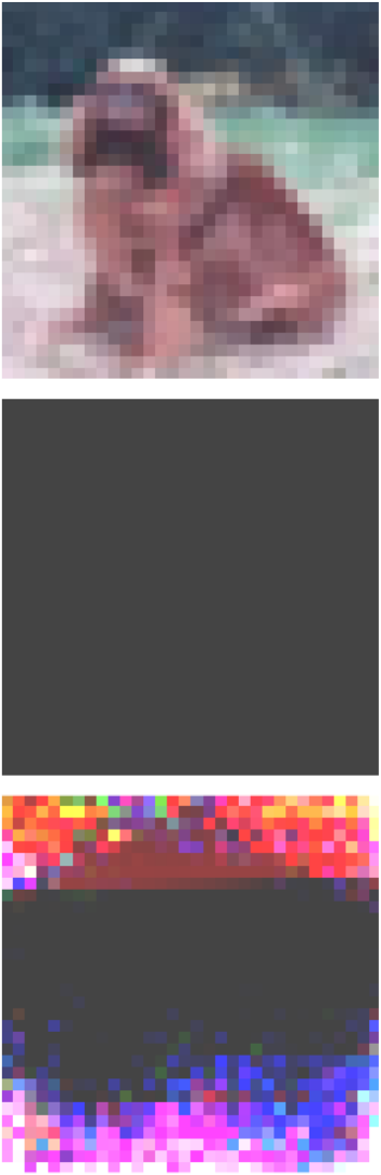
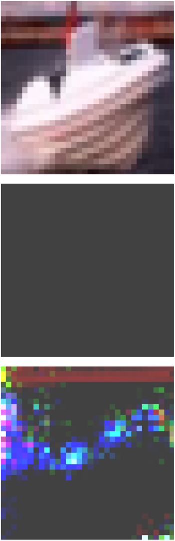
Anisotropic certification allows for a better characterization of the decision boundaries of the base classifier . For example, the directions aligned with the major axes of the ellipsoids , i.e. locations where is large, are, by definition, expected to be less sensitive to perturbations compared to the minor axes directions. To visualize this concept, Figure 15 shows CIFAR-10 images along with their corresponding optimized isotropic parameters obtained by Isotropic DD, and anisotropic parameters obtained by AnCer. First, we note the richness of information provided by the anisotropic parameters when compared to the worst-case, isotropic one. Interestingly, pixel locations where the intensity of is large (higher intensity in Figure 15) are generally the ones corresponding least with the underlying true class and overlapping more with background pixels.
A particular insight one can get from AnCer certification is that the decision boundaries are not distributed isotropically around each input. To quantify this in higher dimensions, we plot in Figure 16 a histogram of the ratio between the maximum and minimum elements of our optimized smoothing parameters for the experiments on SmoothAdv (with an initial ) on CIFAR-10. We note that this ratio can be as high as 5 for some of the input points, meaning the decision boundaries in that case could be 5 times closer to a given input for some directions than others.






Appendix I Non data-dependent Anisotropic Certification
As mentioned briefly in Section 6, it is our intuition that anisotropic certification requires a data-dependent approach, as different points will have fairly different decision boundaries and the certified regions will extend in different directions (as exemplified in Figure 1).
To validate this claim, we perform certification of SmoothAdv Salman et al. 2019a with an initial on CIFAR-10 using a which is the average of all the optimized . The results of the certified accuracy, and are presented in Table 6, along with the same results for the methods reported in the main paper. As can be observed, moving away from the data-dependent certification in the anisotropic scenario leads to a significant performance drop in terms of robustness.
| CIFAR-10 | SmoothAdv | Accuracy @ radius (%) | ||||||||
| 0.0 | 0.25 | 0.5 | 1.0 | 1.5 | 2.0 | 2.5 | ||||
| Fixed | 45 | 40 | 35 | 25 | 16 | 9 | 5 | 0.565 | 0.565 | |
| Isotropic DD | 41 | 39 | 36 | 29 | 21 | 14 | 7 | 0.694 | 0.694 | |
| AnCer | 44 | 43 | 41 | 35 | 26 | 15 | 8 | 0.871 | 0.992 | |
| Average | 29 | 25 | 21 | 14 | 9 | 5 | 2 | 0.329 | 0.379 | |
Appendix J Theoretical and Empirical Comparison with Mohapatra et al. 2020
In regards to the theoretical results, unfortunately the certified regions of Mohapatra et al. 2020 do not exhibit a closed form solution similarly to ours. Thus, a direct theoretical volume bound comparison is not possible.
As for the empirical comparison, AnCer’s performance on both and certificates far out-does that of Mohapatra et al. 2020. For example, with certificates at a radius of , Cohen certified with AnCer achieves certified accuracy (see Table 1) while Mohapatra et al. 2020 achieves under certified accuracy. Note that Mohapatra et al. 2020 has only a marginal improvement over Cohen et al. As for the certificates, Mohapatra et al. 2020 uses the Gaussian distribution of Cohen et al, resulting in worse performance than existing state-of-art in Yang et al. 2020 that uses a uniform distribution. Our approach improves further upon the performance of Yang et al. 2020. For example, as per Table 2, RS4A with ANCER certification achieves certified accuracy at an radius of , Yang et al. 2020 achieves certified accuracy while Mohapatra et al. 2020 achieves below . However, we believe that the combination of both approaches, ANCER and Mohapatra et al. 2020 can further boost the performance as also hinted on in the abstract of Mohapatra et al. 2020 on the use of data-dependent smoothing.