Joint Modeling of Longitudinal and Survival Data with Censored Single-index Varying Coefficient Models
Abstract
In medical and biological research, longitudinal data and survival data types are commonly seen. Traditional statistical models mostly consider to deal with either of the data types, such as linear mixed models for longitudinal data, and the Cox models for survival data, while they do not adjust the association between these two different data types. It is desirable to have a joint modeling approach which accomadates both data types and the dependency between them. In this paper, we extend traditional single-index models to a new joint modeling approach, by replacing the single-index component to a varying coefficient component to deal with longitudinal outcomes, and accomadate the random censoring problem in survival analysis by nonparametric synthetic data regression for the link function. Numerical experiments are conducted to evaluate the finite sample performance.
Index Terms:
Single index model; Varying coefficient model; Survival data; Longitudinal data; Joint modeling.I Introduction
In many medical studies, repeated measurements or longitudinal data are frequently observed, such as patient health outcomes data or biomarker data at sequential visits for each patient [1, 2, 3, 4]. In addition, survival outcomes are usually used as endpoints for clinical evaluations, such as time to disease progression, in particular in cancer trials[5, 6, 7]. Different statistical methods have been proposed to deal with longitudinal data or survival data, respectively. For example, linear mixed models can be used to deal with repeated measurements, and Cox proportional hazard models could be used to deal with survival data. While these traditional models do not consider possible dependency between the two types of data, especially considering the fact that the two different types of data often appear simultaneously, for example, in cancer clinical trials, patient data are collected longitudinally, and progression free survival is often the clinical endpoints[8, 9]. Thus, it is desirable to have statistical methods to accomadate both data types at the same time and account for the dependency, where it is also referred as a ”joint modeling” approach.
In the literature of statistical modeling, single-index models have been extensively studied and discussed as an extension of linear regression models, which retains the interpretability of linear regression models, and enables more model flexibility by imposing a nonparametric link function[11, 12, 13]. Given the popularity of single-index models, in this article, we extend traditional single-index models, and propose a censored single-index varying coefficient model to accomadate for longitudinal and survival data. The longitudinal data type is justified by the varying coefficient component and the survival data type is addressed by the non-parametric link function with a nonparametric synthetic data regression method.
The paper is organized as follows, section II presents the model, the intuition and estimation methods. Section III presents the numerical experiments. Section IV states conclusion and further interest.
II Model and Estimation procedure
II-A Model
Consider the following censored single-index varying coefficient model,
| (1) |
where represents the survival time, is a -dimensional covariate vector, each is an unspecified smooth functions on , is an unknown smooth function, and ’s are random errors. Let be the random censoring time variable associated with the response , and we assume that is independent of . Due to random censoring, we can only observe , where , . Instead of making parametric distributional assumptions such as normality, here we only assume that ’s are independently and identically distributed (i.i.d.) from an unknown distribution symmetric around with finite variance. Furthermore, we assume that no intercept is included in the index function , for each and the first element of is positive, to ensure identifiability, where denotes the norm. In addition, for some compact set .
II-B Estimation of varying coefficient components
Under model (1), the proposed estimation procedure for is inspired by a theorem below.
Assumption A.1 (i) The latent response has first absolute moments. (ii) The density functions of and censoring variable , denoted as and , are continuously differentiable, and is symmetric around zero.
Theorem 1 Let be the distribution function of . Under Assumption A.1, if =0, then
| (2) | |||||
Proof of Theorem 1 could be referred to proof of proposition 1 in [6]. Assumption A.1 and the assumption =0 are mild, and most commonly used distributions, like normal distribution, Student distribution, uniform distribution on a symmetric interval, satisfy these assumptions [6]. Theorem 1 implies that can be represented as a new model with the same varying coefficient functions , but a new link function, i.e., , where ’’ means composition of two functions and
By Theorem 1, we give a new single-index varying coefficient for the observed response as
| (3) |
where , satisfying given Assumption A.1. By re-expressing our orginal model into (3), a general estimation method for single-index varying coefficient models can be applied to estimate . We adopt the Least-Squares type method in [14] to estimate , denoted as .
II-C Nonparametric synthetic data regression of
With estimated in hand, we now move to discuss the estimation of the unknown link function . Let . To begin, we re-express model(1) as (4). With estimates in hand, we now estimate the unknown link function . To begin, we re-express model (1) as
| (4) |
where . Therefore, we have an one dimensional nonparametric randomly censored regression model with predictor variable , traditional methods like [15, 16] can be used to estimate . For computational and theoretical convenient, we adopt the method in [16] and give the following estimating procedure for . Let , and define the synthetic transformation of response variable as
where is the Kaplan-Meier estimator of the survival function . After transformation, usual kernel smoothing can be applied to observations to estimate the link function . The Nadaraya-Watson kernel estimator of based on the synthetic data is given by
where , the Rosenblatt-Parzen estimator of . And , where is a -variate kernel function. The bandwidth selection follows the same pattern as in [14].
III Simulation study
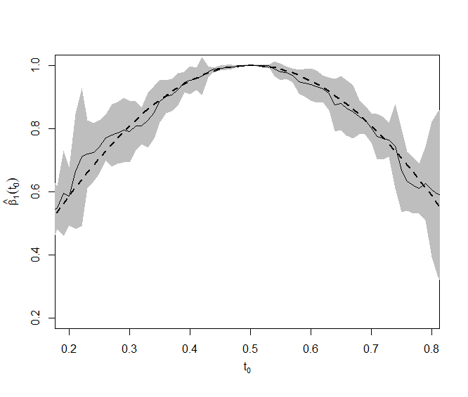
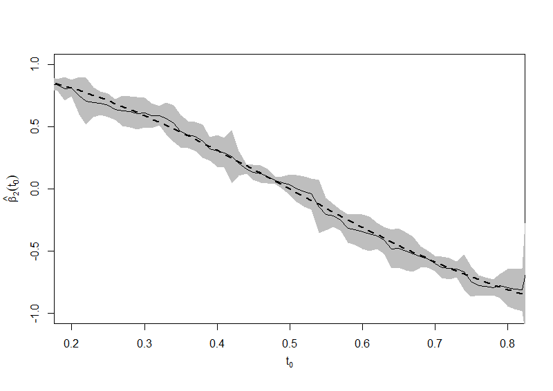
In this section, we investigate the finite sample performance of our proposed estimation by Monte Carlo simulations. We generated random samples of size responses from model with two covariates. We took to be to be independent standard normal covariates. The effect modifier is taken to be a uniform random variable over and , independent of both and . The data are generated from model(1): and , were taken to be and . . Choose such that the censoring level is . In order to assess the pointwise variability of the coefficient function estimators, we plotted the 5th and the 95th pointwise percentiles of the 100 estimates of our estimated coefficient functions. Figure 1 presents the point-wise median curve of the estimated functions and on the grid points uniformly spaced between , point-wise 5% quantile and 95 % quantile of and . In general, the fitted values (solid lines) are close to the true values (dashed lines), and the confidence bands covers the true function except for some small region. And Figure 2 presents the point-wise median curve of the estimated function n the grid points uniformly spaced between , with 5% quantile and 95 % quantile of , it can be seen that it assembles a quadratic function.

IV Conclusions
In this research article, we proposed a new censored single-index varing coefficient model as a tool for joint modeling of longitudinal and survival data.Varying coefficient index adjusts for the longitudinal effect and the non-parametric link function accounts for random censoring problem. The intuition of the method was stated and numerical experiments were examined. In the future, research directions would be in asymptotic properties and real data examples.
References
- [1] C. Orkin, E. DeJesus, P. E. Sax, J. R. Arribas, S. K. Gupta, C. Martorell, J. L. Stephens, H.-J. Stellbrink, D. Wohl, F. Maggiolo, M. A. Thompson, D. Podzamczer, D. Hagins, J. A. Flamm, C. Brinson, A. Clarke, H. Huang, R. Acosta, D. M. Brainard, S. E. Collins, and H. Martin, “Fixed-dose combination bictegravir, emtricitabine, and tenofovir alafenamide versus dolutegravir-containing regimens for initial treatment of hiv-1 infection: week 144 results from two randomised, double-blind, multicentre, phase 3, non-inferiority trials,” The Lancet HIV, vol. 7, no. 6, pp. e389–e400, 2020. [Online]. Available: https://www.sciencedirect.com/science/article/pii/S2352301820300990
- [2] H. Huang, Y. Li, H. Liang, and C. O. Wu, “Decomposition feature selection with applications in detecting correlated biomarkers of bipolar disorders,” Statistics in medicine, vol. 38, no. 23, pp. 4574–4582, 2019.
- [3] K. M. Erlandson, C. C. Carter, K. Melbourne, T. T. Brown, C. Cohen, M. Das, S. Esser, H. Huang, J. R. Koethe, H. Martin et al., “Weight change following antiretroviral therapy switch in people with viral suppression: Pooled data from randomized clinical trials,” Clinical Infectious Diseases, 2021.
- [4] R. K. Acosta, G. Q. Chen, S. Chang, R. Martin, X. Wang, H. Huang, D. Brainard, S. E. Collins, H. Martin, and K. L. White, “Three-year study of pre-existing drug resistance substitutions and efficacy of bictegravir/emtricitabine/tenofovir alafenamide in hiv-1 treatment-naive participants,” Journal of Antimicrobial Chemotherapy, 2021.
- [5] H. Huang, J. Shangguan, P. Ruan, and H. Liang, “Bi-level feature selection in high dimensional aft models with applications to a genomic study,” Statistical applications in genetics and molecular biology, vol. 18, no. 5, 2019.
- [6] H. Huang, J. Shangguan, X. Li, and H. Liang, “High-dimensional single-index models with censored responses,” Statistics in medicine, vol. 39, no. 21, pp. 2743–2754, 2020.
- [7] A. Castagna, D. S. C. Hui, K. M. Mullane, K. M. Mullane, M. Jain, M. Galli, S.-C. Chang, R. H. Hyland, D. SenGupta, H. Cao et al., “548. baseline characteristics associated with clinical improvement and mortality in hospitalized patients with moderate covid-19,” in Open Forum Infectious Diseases, vol. 7, no. Supplement_1. Oxford University Press US, 2020, pp. S340–S340.
- [8] J. G. Ibrahim, H. Chu, and L. M. Chen, “Basic concepts and methods for joint models of longitudinal and survival data,” Journal of Clinical Oncology, vol. 28, no. 16, p. 2796, 2010.
- [9] H. Huang, Y. Tang, Y. Li, and H. Liang, “Estimation in additive models with fixed censored responses,” Journal of Nonparametric Statistics, vol. 31, no. 1, pp. 131–143, 2019.
- [10] H. Huang, “Novel semi-parametric tobit additive regression models,” arXiv preprint arXiv:2107.01497, 2021.
- [11] H. Huang, Y. Li, H. Liang, and Y. Tang, “Estimation of single-index models with fixed censored responses,” Statistica Sinica, vol. 30, no. 2, pp. 829–843, 2020.
- [12] H. Huang, J. Shangguan, Y. Li, and H. Liang, “Bi-level variable selection in high-dimensional tobit models,” Statistics and Its Interface, vol. 13, no. 2, pp. 151–156, 2020.
- [13] H. Huang, “Semi-parametric and structured nonparametric modeling with censored responses,” Ph.D. dissertation, The George Washington University, 2017.
- [14] C. Kuruwita, K. Kulasekera, and C. Gallagher, “Generalized varying coefficient models with unknown link function,” Biometrika, vol. 98, no. 3, pp. 701–710, 2011.
- [15] J. Fan and I. Gijbels, “Censored regression: local linear approximations and their applications,” Journal of the American Statistical Association, vol. 89, no. 426, pp. 560–570, 1994.
- [16] H. Koul, V. Susarla, J. Van Ryzin et al., “Regression analysis with randomly right-censored data,” Annals of statistics, vol. 9, no. 6, pp. 1276–1288, 1981.