A Differential Private Method for Distributed Optimization in Directed Networks via State Decomposition

Xiaomeng Chen Affiliation: X. Chen, L. Huang and L. Shi are with the Department of Electronic and Computer Engineering, Hong Kong University of Science and Technology, Clear Water Bay, Kowloon, Hong Kong ( email:xchendu@connect.ust.hk, lhuangaq@connect.ust.hk, eesling@ust.hk). Lingying Huang Affiliation: X. Chen, L. Huang and L. Shi are with the Department of Electronic and Computer Engineering, Hong Kong University of Science and Technology, Clear Water Bay, Kowloon, Hong Kong ( email:xchendu@connect.ust.hk, lhuangaq@connect.ust.hk, eesling@ust.hk). Affiliation: L. He is with the school of Automation at Nanjing University of Science and Technology, P. R. China, 210094 (email: lidonghe@njust.edu.cn). Lidong He Affiliation: S. Dey is with the Hamilton Institute, NUI Maynooth, Maynooth, Co. Kildare, Ireland, and also affiliated with Uppsala University. (email: subhrakanti.dey@angstrom.uu.se). Subhrakanti Dey Ling Shi Affiliation: X. Chen, L. Huang and L. Shi are with the Department of Electronic and Computer Engineering, Hong Kong University of Science and Technology, Clear Water Bay, Kowloon, Hong Kong ( email:xchendu@connect.ust.hk, lhuangaq@connect.ust.hk, eesling@ust.hk).

Abstract

In this paper, we study the problem of consensus-based distributed optimization, where a network of agents, abstracted as a directed graph, aims to minimize the sum of all agents’ cost functions collaboratively. In existing distributed optimization approaches (Push-Pull/AB) for directed graphs, all agents exchange their states with neighbors to achieve the optimal solution with a constant stepsize, which may lead to the disclosure of sensitive and private information. For privacy preservation, we propose a novel state-decomposition based gradient tracking approach (SD-Push-Pull) for distributed optimzation over directed networks that preserves differential privacy, which is a strong notion that protects agents’ privacy against an adversary with arbitrary auxiliary information. The main idea of the proposed approach is to decompose the gradient state of each agent into two sub-states. Only one substate is exchanged by the agent with its neighbours over time, and the other one is not shared. That is to say, only one substate is visible to an adversary, protecting the sensitive information from being leaked. It is proved that under certain decomposition principles, a bound for the sub-optimality of the proposed algorithm can be derived and the differential privacy is achieved simultaneously. Moreover, the trade-off between differential privacy and the optimization accuracy is also characterized. Finally, a numerical simulation is provided to illustrate the effectiveness of the proposed approach.

Index Terms:

distributed optimization, directed graph, decomposition, differential private.

I INTRODUCTION

With the rapid development in networking technologies, distributed optimization over multi-agent networks has been a heated research topic during the last decade, where agents aim to collaboratively minimize the sum of local functions possessed by each agent through local communication. Compared with centralized ones, distributed algorithms allow more flexibility and scalability due to its capability of breaking large-scale problems into sequences of smaller ones. In view of this, distributed algorithms are inherently robust to environment uncertainties and communication failures and are widely adopted in power grids [1], sensor networks [2] and vehicular networks [3].

The most commonly used algorithms for distributed optimization is the Decentralized Gradient Descent (DGD), requiring diminishing step-sizes to ensure optimality [4]. To overcome this challenge, Xu et al.[5] replaced the local gradient with an estimated global gradient based on the dynamic average consensus [6] and then proposed a gradient tracking method for distributed optimzation problem. Recently, Pu et al. [7] and Xin and Khan [8] devised a modified gradient-tracking algorithm called Push-Pull/AB algorithm for consensus-based distributed optimization, which can be applied to a general directed graph including undirected graph as a special case.
The above conventional distributed algorithms require each agent to exchange their state information with the neighbouring agent, which is not desirable if the participating agents have sensitive and private information, as the transmitted information is at risk of being intercepted by adversaries. By hacking into communication links, an adversary may have access to all conveyed messages, and potentially obtain the private information of each agent by adopting an attack algorithm. The theoretical analysis of privacy disclosure in distributed optimization is presented by Mandal[9], where the parameters of cost functions and generation power can be correctly inferred by an eavesdropper in the economic dispatch problem. As the number of privacy leakage events is increasing, there is an urgent need to preserve privacy of each agent in distributed systems.
For the privacy preservation in distributed optimization, there have been several research results. Wang[10] proposed a privacy-preserving average consensus in which the state of an agent is decomposed into two substates. Zhang et al. [11] and Lu et al. [12] combined existing distributed optimization approaches with the partially homomorphic cryptography. However, these approaches suffer from high computation complexity and communication cost which may be inapplicable for systems with limited resources. As an appealing alternative, differential privacy has attracted much attention in light of its rigorous mathematical framework, proven security properties, and easy implementation [13]. The main idea of differential private approaches is noise perturbation, leading to a tradeoff between privacy and accuracy. Huang et al. [14] devised a differential private distributed optimization algorithm by adding Laplacian noise on transmitted message with a decaying stepsize, resulting in a low convergence rate. A constant stepsize is achieved by Ding et al. [15, 16] where linear convergence is enjoyed by gradient tracking method and differential privacy is achieved by perturbing states.

None of the aforementioned approaches, however, is suitable for directed graphs with weak topological restrictions, which is more practical in real applications. In practice, the information flows among sensors may not be bidirectional due to the different communication ranges, e.g., the coordinated vechicle control problem [17] and the economic dispatch problem [18]. To address privacy leakage in distributed optimization for agents interacting over an unbalanced graphs, Mao et al. [19] designed a privacy-preserving algorithm based on the push-gradient method with a decaying stepsize, which is implemented via a case study to the economic dispatch problem. Nevertheless, the algorithm in [19] lacked a formal privacy notion and it cannot achieve differential privacy.
All the above motivates us to further develop a differential private distributed optimization algorithm over directed graphs. Inspired by [10], a novel differential private distributed optimization approach based on state decomposition is proposed for agents communicating over directed networks. Under the proposed state decomposition mechanism, a Laplacian noise is perturbed on the gradient state and the global gradient is still tracked after state decomposition. The main contributions of this paper are summarized as follows:

1.

We propose a state-decomposition based gradient tracking approach (SD-Push-Pull) for distributed optimziation over unbalanced directed networks, where the gradient state of each agent is decomposed into two substates to maintain the privacy of all agents. Specifically, one sub-state replacing the role of the original state is communicated with neighboring agents while the other substate is not shared. Compared to the privacy-preserving approaches in [14] and [15], our proposed approach can be applied to more general and practical networks.
2.

By carefully designing the state decomposition mechanism, we only need to add noise to one substate of directions instead of perturbing both states and directions [16]. Moreover, our proposed SD-Push-Pull algorithm does not require the stepsize or noise variance to be diminishing, which ensures a linear convergence to a neighborhood of the optimal solution in expectation exponentially fast under a constant stepsize policy (Theorem 1).
3.

Different from the privacy notion in [10] and [19], we adopt the definition of differential privacy, which ensures the privacy of agents regardless of any auxiliary information that an adversary may have and enjoys a rigorous formulation. In addition, we prove that the proposed SD-Push-Pull algorithm can achieve $\epsilon$ -differential privacy (Theorem 2).

Notations: In this paper, $\mathbb{N}$ and $\mathbb{R}$ represent the sets whose components are natural numbers and real numbers. $\mathbb{R}_{++}$ denotes the set of all positive real numbers. $\mathbb{R}^{n}$ and $\mathbb{R}^{n\times p}$ represent the set of $n-$ dimensional vectors and $n\times p$ -dimensional matrices. We let $(\mathbb{R}^{n\times p})^{\mathbb{N}}$ denote the space of vector-valued sequences in $\mathbb{R}^{n\times p}$ . $\mathbf{1}_{n}\in\mathbb{R}^{n}$ and $\mathbf{I}_{n}\in\mathbb{R}^{n\times n}$ represent the vector of ones and the identity matrix, respectively. The spectral radius of matrix $\mathbf{A}$ is denoted by $\rho(\mathbf{A})$ . $[\mathbf{x}]_{r}$ denotes the $r-$ th element of the vector $\mathbf{x}$ . For a given constant $\theta>0$ , Lap( $\theta$ ) is the Laplace distribution with probability function $f_{L}(x,\theta)=\frac{1}{2\theta}e^{-\frac{|x|}{\theta}}$ . In addition, $\mathbb{E}(x)$ and $P(x)$ denote the expectation and probability distribution of a random variable $x$ , respectively.

II PRELIMINARIES AND PROBLEM FORMULATION

II-A Network Model

We consider a group of agents which communicate with each other over a directed graph. The directed graph is denoted as a pair $G\triangleq(\mathcal{N},\mathcal{E})$ , where $\mathcal{N}$ denotes the agents set and $\mathcal{E}\subset\mathcal{N}\times\mathcal{N}$ denotes the edge set, respectively. A communication link from agent $i$ to agent $j$ is denoted by $(j,i)\in\mathcal{E}$ , indicating that agent $i$ can send messages to agent $j$ . Given a nonnegative matrix $\mathbf{M}=[m_{ij}]\in\mathbb{R}^{n\times n}$ , the directed graph induced by $\mathbf{M}$ is denoted by $\mathcal{G}_{\mathbf{M}}\triangleq(\mathcal{N},\mathcal{E}_{\mathbf{M}})$ , where $\mathcal{N}=\{1,2,\ldots,n\}$ and $(j,i)\in\mathcal{E}_{\mathbf{M}}$ if and only if $m_{ij}>0$ . The agents who can directly send messages to agent $i$ are represented as in-neighbours of agent $i$ and the set of these agents is denoted as $N_{\mathbf{M},i}^{in}=\{j\in\mathcal{N}\mid(i,j)\in\mathcal{E}_{\mathbf{M}}\}$ . Similarly, the agents who can directly receive messages from agent $i$ are represented as out-neighbours of agent $i$ and the set of these agents is denoted as $N_{\mathbf{M},i}^{out}=\{j\in\mathcal{N}\mid(j,i)\in\mathcal{E}_{\mathbf{M}}\}$ .

II-B Differential Privacy

Differential privacy serves as a mathematical notion which quantify the degree of the involved individuals’ privacy guarantee in a statistical database. We give the following definitions for preliminaries of differential privacy in distributed optimization.

Definition 1

(Adjacency [20]) Two function sets $\mathcal{S}^{(1)}=\{f_{i}^{(1)}\}^{n}_{i=1}$ and $\mathcal{S}^{(2)}=\{f_{i}^{(2)}\}^{n}_{i=1}$ , $\mathcal{S}^{(1)}$ and $\mathcal{S}^{(2)}$ are said to be adjacent if there exists some $i_{0}\in\{1,2\ldots,n\}$ such that $f_{i}^{(1)}=f_{i}^{(2)},\forall i\neq i_{0}$ and $f_{i_{0}}^{(1)}\neq f_{i_{0}}^{(2)}$ .

Definition 1 implies that two function sets are adjacent only if one agent changes its objective function.

Definition 2

(Differential privacy [21]) Given $\epsilon>0,$ for any pair of adjacent function sets $\mathcal{S}^{(1)}$ and $\mathcal{S}^{(2)}$ and any observation $\mathcal{O}\subseteq\text{Range}(\mathcal{A})$ , a randomized algorithm $\mathcal{A}$ keeps $\epsilon-$ differentially private if

P\{\mathcal{A}(\mathcal{S}^{(1)})\in\mathcal{O}\}\leq e^{\epsilon}P\{\mathcal{A}(\mathcal{S}^{(2)})\in\mathcal{O}\}

where $\text{Range}(\mathcal{A})$ denotes the output codomain of $\mathcal{A}$ .

Definition 2 illustrates that a random mechanism is differentially private if its outputs are nearly statistically identical over two similar inputs which only differ in one element. Hence, an eavesdropper cannot distinguish between two function sets with high probability based on the output of the mechanism. Here, a smaller $\epsilon$ represents a higher level of privacy since the eavesdropper has less chance to distinguish sensitive information of each agent from the observations. Nevertheless, a high privacy level will sacrifice the accuracy of the optimization algorithm. Hence, the constant $\epsilon$ determines a tradeoff between the privacy level and the accuracy.

II-C Problem Formulation

Consider an optimization problem in a multi-agent system of $n$ agents. Each agent has a private cost function $f_{i}$ , which is only known to agent $i$ itself. All the participating agents aim to minimize a global objective function

\min\limits_{x\in\mathbb{R}^{p}}\sum\limits_{i=1}^{n}f_{i}(x)

(1)

where $x$ is the global decision variable.

To solve Problem (1), assume each agent $i$ maintains a local copy of $x_{i}\in\mathbb{R}^{p}$ of the decision variable and an auxiliary variable $y_{i}\in\mathbb{R}^{p}$ tracking the average gradients. Then we can rewrite Problem (1) into local optimization problem of each agent with an added consensus constraint as follows

\begin{split}\min_{x_{i}\in\mathbb{R}^{p}}\quad&\sum_{i=1}^{n}f_{i}(x_{i})\\ \text{s.t.}\quad&x_{i}=x_{j},\quad\forall i,j,\\ \end{split}

(2)

where $x_{i}$ is the local decision variable of the agent $i$ .

Let

		$\displaystyle\mathbf{x}:=[x_{1},x_{2},\ldots,x_{n}]^{\top}\in\mathbb{R}^{n\times p},$
		$\displaystyle\mathbf{y}:=[y_{1},y_{2},\ldots,y_{n}]^{\top}\in\mathbb{R}^{n\times p}.$

Denote $F(x)$ as an aggregate objective function of the local variables, i.e., $F(x)=\sum_{i=1}^{n}f_{i}(x_{i})$ .

With respect to the objective function in Problem (1), we assume the following strong convexity and smoothness conditions.

Assumption 1

Each objective function $f_{i}$ is $\mu-$ strongly convex with $L-$ Lipschitz continuous gradients, i.e., for any $\mathbf{x}$ , $\mathbf{y}\in\mathbb{R}^{p}$ ,

		$\displaystyle\langle\nabla f_{i}(\mathbf{x})-\nabla f_{i}(\mathbf{y}),\mathbf{x}-\mathbf{y}\rangle\geq\mu\|\|\mathbf{x}-\mathbf{y}\|\|^{2},$
		$\displaystyle\|\|\nabla f_{i}(\mathbf{x})-\nabla f_{i}(\mathbf{y})\|\|\leq L\|\|\mathbf{x}-\mathbf{y}\|\|.$

Under Assumption 1, Problem (1) has a unique optimal solution $x^{\star}\in\mathbb{R}^{p}$ [22].

III PRIVATE GRADIENT TRACKING ALGORITHM VIA STATE DECOMPOISTION

In this section, we propose a state-decomposition based gradient tracking method (SD-Push-Pull) for distributed optimization over directed graphs, which is described in Algorithm III. The main idea is to let each agent decompose its gradient state $y_{i}$ into two substates $y^{\alpha}_{i}$ and $y^{\beta}_{i}$ . The substate $y^{\alpha}_{i}$ is used in the communication with other agents while $y^{\beta}_{i}$ is never shared with other agents except for agent $i$ itself, so the substate $y^{\beta}_{i}$ is imperceptible to the neighbouring agents of agent $i$ .

Algorithm 1 SD-Push-Pull

Step 1. Initialization:

1.

Agent $i\in\mathcal{N}$ chooses in-bound mixing/pulling weights $R_{ij}\geq 0$ for all $j\in N^{in}_{R,i}$ , out-bound pushing weights $\tilde{C}_{li}\geq 0$ for all $l\in N^{out}_{\tilde{C},i}$ , and the two sub-state weights $\alpha_{i},\beta_{i}\in(0,1)$ .
2.

Agent $i\in\mathcal{N}$ picks any $x_{i,0},y_{i,0}^{\alpha},y_{i,0}^{\beta}\in\mathbb{R}^{p},$ $\theta_{i}\in\mathbb{R_{++}}$ .
3.

The step size $\eta>0$ is known to each agent.

Step 2. At iteration

k=0,1,2,\ldots,{\color[rgb]{0,0,0}K}

1. Agent

i\in\mathcal{N}

pushes

\tilde{C}_{li}y_{i,k}^{\alpha}

to each

l\in N^{out}_{\tilde{C},i}

. 2. Agent

i\in\mathcal{N}

draws a random vector

\xi_{i,k}

consisting of

p

Laplacian noise independently drawn from Lap(

\theta_{i}

) and updates

y_{i,k+1}^{\alpha}

y_{i,k+1}^{\beta}

as follows:

\displaystyle y_{i,k+1}^{\alpha}=\sum_{j\in N^{in}_{\tilde{C},i}\cup\{i\}}\tilde{C}_{ij}y_{j,k}^{\alpha}+(1-\beta_{i})y_{i,k}^{\beta}+\xi_{i,k}

(3a)

\displaystyle y_{i,k+1}^{\beta}=\alpha_{i}y_{i,k}^{\alpha}+\beta_{i}y_{i,k}^{\beta}+\nabla f_{i}(x_{i,k})

(3b) 3. Agent

i\in\mathcal{N}

pulls

[x_{j,k}-\eta(y_{j,k+1}^{\alpha}-y_{j,k}^{\alpha})]

from each

j\in N^{in}_{R,i}

. 4. Agent

i\in\mathcal{N}

updates

x_{i,k+1}

through

x_{i,k+1}=\sum_{j\in N^{in}_{R,i}\cup\{i\}}R_{ij}[x_{j,k}-\eta(y_{j,k+1}^{\alpha}-y_{j,k}^{\alpha})].

(4)

Denote

		$\displaystyle\mathbf{R}:=[R_{ij}],\quad\mathbf{\Lambda_{\alpha}}:=diag(\alpha_{1},\alpha_{2},\ldots,\alpha_{n}),$
		$\displaystyle\mathbf{\tilde{C}}:=[\tilde{C}_{ij}],\quad\mathbf{\Lambda_{\beta}}:=diag(\beta_{1},\beta_{2},\ldots,\beta_{n}),$
		$\displaystyle\color[rgb]{0,0,0}{\displaystyle\mathbf{\xi}_{k}:=[\xi_{1,k},\xi_{2,k}\ldots,\xi_{n,k}]^{\top}},$
		$\displaystyle\mathbf{y}_{k}:=[y_{1,k}^{\alpha},\ldots,y_{n,k}^{\alpha}(k),y_{1,k}^{\beta}(k),\ldots,y_{n,k}^{\beta}(k)]^{\top}$
		$\displaystyle\nabla F(\mathbf{x}_{k})=[\nabla f_{1}(x_{1,k}),\ldots,\nabla f_{n}(x_{n,k})]^{\top},$
		$\displaystyle\color[rgb]{0,0,0}{\displaystyle\nabla{\tilde{F}}(\mathbf{x}_{k})=[\mathbf{\xi}_{k}^{\top},\nabla F(\mathbf{x}_{k})^{\top}]^{\top},}$
		$\displaystyle\mathbf{C}:=\begin{bmatrix}\mathbf{\tilde{C}}&\bf{I}_{n}-\mathbf{\Lambda_{\beta}}\\ \mathbf{\Lambda_{\alpha}}&\mathbf{\Lambda_{\beta}}\\ \end{bmatrix},\quad\mathbf{T}:=\begin{bmatrix}\mathbf{I}_{n}&\mathbf{0}_{n}\end{bmatrix}.$

Algorithm III can be rewritten in a matrix form as follows:


	$\displaystyle\mathbf{y}_{k+1}=\mathbf{C}\mathbf{y}_{k}+\nabla{\tilde{F}}(\mathbf{x}_{k}),$	(5a)
	$\displaystyle\mathbf{x}_{k+1}=\mathbf{R}[\mathbf{x}_{k}-\eta\mathbf{T}(\mathbf{y}_{k+1}-\mathbf{y}_{k})],$	(5b)
where $\mathbf{x}_{0}$ and $\mathbf{y}_{0}$ are arbitrary.

Remark 1

In SD-Push-Pull, we design a state decomposition mechanism for the direction state (shown in (3)), where sensitive information $\nabla f_{i}(x_{i,k})$ is contained in one substate of direction, $y_{i,k+1}^{\beta}$ . Since the substate $y_{i,k+1}^{\beta}$ is not shared in communication link, the private information $\nabla f_{i}(x_{i,k})$ of agent $i$ is protected from being leaked. Although $y_{i,k}^{\beta}$ will be shared through $y_{i,k+1}^{\alpha}$ , the noise $\xi_{i,k}$ added in the updated of $y_{i,k}^{\alpha}$ (shown in (3a)) helps to avoid privacy breaches of $f_{i}$ . The above discussion intuitively illustrates how state decomposition mechanism achieves differential privacy of each agent. Rigorous theoretical analysis will be provided in Section V.

Assumption 2

The matrix $\mathbf{R}\in\mathbb{R}^{n\times n}$ is a nonnegative row-stochastic matrix and $\mathbf{C}\in\mathbb{R}^{2n\times 2n}$ is a nonnegative column-stochastic matrix, i.e., $\mathbf{R1}_{n}=\mathbf{1}_{n}$ and $\mathbf{1}_{2n}^{\top}\mathbf{C}=\mathbf{1}_{2n}^{\top}$ . Moreover, the diagonal entries of $\mathbf{R}$ and $\mathbf{C}$ are positive, i.e., $R_{ii}>0,\tilde{C}_{ii}>0,\forall i\in\mathcal{N}$ .

Assumption 2 can be satisfied by properly designing the weights in $\mathbf{R}$ and $\mathbf{C}$ by each agent locally. For instance, each agent may choose $R_{ij}=\frac{1}{|N^{in}_{R,i}|+c_{R}}$ for some constant $c_{R}>0$ for all $j\in N^{in}_{R,i}$ and let $R_{ii}=1-\sum_{j\in N^{in}_{R,i}}R_{ij}$ . Similarly, agent $i$ may choose $\alpha_{i}=\zeta$ and $\tilde{C}_{li}=\frac{1-\zeta}{|N^{out}_{C,i}|+c_{C}}$ for some constant $0<\zeta<1,c_{C}>0$ for all $l\in N^{out}_{C,i}$ , and let $\tilde{C}_{ii}=1-\zeta-\sum_{l\in N^{out}_{C,i}}\tilde{C}_{li}$ . Such a choice of weights renders $\mathbf{R}$ row-stochastic and $\mathbf{C}$ column-stochastic, thus satisfying Assumption 2.

Assumption 3

The graphs $\mathcal{G}_{\mathbf{R}}$ and $\mathcal{G}_{\mathbf{C^{\top}}}$ induced by matrices $\mathbf{R}$ and $\mathbf{C}$ contain at least one spanning tree. In addition, there exists at least one agent that is a root of spanning trees for both $\mathcal{G}_{\mathbf{R}}$ and $\mathcal{G}_{\mathbf{C^{\top}}}$ .

Assumption 3 is weaker than assumptions in most previous works (e.g.,[8], [23], [24]), where graphs $\mathcal{G}_{\mathbf{R}}$ and $\mathcal{G}_{\mathbf{C^{\top}}}$ are assumed to be strongly connected. The relaxed assumption about graph topology enables us to design graphs $\mathcal{G}_{\mathbf{R}}$ and $\mathcal{G}_{\mathbf{C^{\top}}}$ more flexibly. Similar assumption are adopted in [22], [25].

Lemma 1 ([26])

Under Assumption 2-3, the matrix $\mathbf{R}$ has a unique nonnegative left eigenvector $u^{\top}$ (w.r.t. eigenvalue) with $u^{\top}\mathbf{1}_{n}=n,$ and matrix $\mathbf{C}$ has a unique nonnegative right eigenvector $v$ (w.r.t. eigenvalue) with $\mathbf{1}_{2n}^{\top}v=n$ .

To make connections with the traditional push-pull algorithm, we let $\mathbf{\tilde{y}}_{k}:=\mathbf{y}_{k+1}-\mathbf{y}_{k}$ . Then one can have


		$\displaystyle\mathbf{x}_{k+1}=\mathbf{R}(\mathbf{x}_{k}-\eta\mathbf{T}\mathbf{\tilde{y}}_{k}),$		(6a)
		$\displaystyle\mathbf{\tilde{y}}_{k+1}=\mathbf{C}\mathbf{\tilde{y}}_{k}+\nabla{\tilde{F}}(\mathbf{x}_{k+1})-\nabla{\tilde{F}}(\mathbf{x}_{k}).$		(6b)

Since $C$ is column stochastic,

\mathbf{1}_{2n}^{\top}\mathbf{\tilde{y}}_{k+1}=\mathbf{1}_{2n}^{\top}\mathbf{\tilde{y}}_{k}+\mathbf{1}_{2n}^{\top}\nabla{\tilde{F}}(\mathbf{x}_{k+1})-\mathbf{1}_{2n}^{\top}\nabla{\tilde{F}}(\mathbf{x}_{k}).

From $\mathbf{1}_{2n}^{\top}\mathbf{\tilde{y}}_{0}=\mathbf{1}_{2n}^{\top}\mathbf{y}_{1}-\mathbf{1}_{2n}^{\top}\mathbf{y}_{0}=\mathbf{1}_{2n}^{\top}\nabla\tilde{F}(\mathbf{x}_{0})$ , we have by induction that

\frac{1}{n}\mathbf{1}_{2n}^{\top}\mathbf{\tilde{y}}_{k}={\color[rgb]{0,0,0}\frac{1}{n}\mathbf{1}_{2n}^{\top}}\nabla\tilde{F}(\mathbf{x}_{k})=\frac{1}{n}\mathbf{1}_{n}^{\top}\nabla F(\mathbf{x}_{k})+\frac{1}{n}\mathbf{1}_{n}^{\top}\mathbf{\xi}_{k}.

(7)

IV Convergence Analysis

In this section, we analyze the convergence performance of the proposed private push-pull algorithm. For the sake of analysis, we define the following variables:

\bar{x}_{k}:=\frac{1}{n}u^{\top}\mathbf{x}_{k},\qquad\bar{y}_{k}=\frac{1}{n}\mathbf{1}_{2n}^{\top}\mathbf{\tilde{y}}_{k}.

The main idea of our strategy is to bound $\mathbb{E}[||\bar{x}_{k+1}-x^{\star\top}||]_{2},\mathbb{E}[||\mathbf{x}_{k+1}-\mathbf{1}_{n}\bar{x}_{k+1}||_{R}],\mathbb{E}[||\mathbf{\tilde{y}}_{k+1}-v\bar{y}_{k+1}]||_{C}]$ on the basis of the linear combinations of their previous values, where $||\cdot||_{R}$ and $||\cdot||_{C}$ are specific norms to be defined later. By establishing a linear system of inequalities, we can derive the convergence result.

Definition 3

Given an arbitrary vector norm $||\cdot||$ , for any $\mathbf{x}\in\mathbb{R}^{n\times p}$ , we define a matrix norm

||\mathbf{x}||:=\Big|\Big|\Big[||\mathbf{x}^{(1)}||,||\mathbf{x}^{(2)}||,\ldots,||\mathbf{x}^{(p)}||\Big]\Big|\Big|_{2}

where $\mathbf{x}^{(1)},\mathbf{x}^{(2)},\ldots,\mathbf{x}^{(p)}\in\mathbb{R}^{n}$ are columns of $\mathbf{x}$ .

IV-A Preliminary Analysis

From Eqs. (6a) and Lemma 1, we can obtain

\bar{x}_{k+1}=\frac{1}{n}u^{\top}\mathbf{R}(\mathbf{x}_{k}-\eta\mathbf{T}\mathbf{\tilde{y}}_{k})=\bar{x}_{k}-\frac{\eta}{n}u^{\top}\mathbf{T}\mathbf{\tilde{y}}_{k}.

(8)

Furthermore, let us define

g_{k}:=\frac{1}{n}\sum_{i=1}^{n}\nabla f_{i}(\bar{x}_{k}),\quad h_{k}:=\frac{1}{n}\sum_{i=1}^{n}\nabla f_{i}(x_{i,k}),

which leads to $\bar{y}_{k}=h_{k}+\frac{1}{n}\mathbf{1}_{n}^{\top}\mathbf{\xi}_{k}.$ Then, from equation (8)

$\displaystyle\bar{x}_{k+1}=$	$\displaystyle\bar{x}_{k}-\frac{\eta}{n}u^{\top}\mathbf{T}(\mathbf{\tilde{y}}_{k}-v\bar{y}_{k}+v\bar{y}_{k})$	(9)
$\displaystyle=$	$\displaystyle\bar{x}_{k}-\frac{\eta}{n}u^{\top}\mathbf{T}v\bar{y}_{k}-\frac{\eta}{n}u^{\top}\mathbf{T}(\mathbf{\tilde{y}}_{k}-v\bar{y}_{k})$
$\displaystyle=$	$\displaystyle\color[rgb]{0,0,0}{\displaystyle\bar{x}_{k}-\eta^{\prime}g_{k}-\eta^{\prime}(h_{k}-g_{k})-\frac{\eta}{n}u^{\top}\mathbf{T}(\mathbf{\tilde{y}}_{k}-v\bar{y}_{k})}$
	$\displaystyle\color[rgb]{0,0,0}{\displaystyle-\frac{\eta^{\prime}}{n}\mathbf{1}_{n}^{\top}\mathbf{\xi}_{k},}$

where $\eta^{\prime}:=\frac{\eta}{n}u^{\top}\mathbf{T}v.$

Based on Lemma 1 and equation (8), we obtain

		$\displaystyle\mathbf{x}_{k+1}-\mathbf{1}_{n}\bar{x}_{k+1}$		(10)
		$\displaystyle=\mathbf{R}(\mathbf{x}_{k}-\eta\mathbf{T}\mathbf{\tilde{y}}_{k})-\mathbf{1}_{n}\bar{x}_{k}+\frac{\eta}{n}\mathbf{1}_{n}u^{\top}\mathbf{T}\mathbf{\tilde{y}}_{k}$
		$\displaystyle=\mathbf{R}(\mathbf{x}_{k}-\mathbf{1}_{n}\bar{x}_{k})-(\mathbf{R}-\frac{\mathbf{1}_{n}u^{\top}}{n})\eta\mathbf{T}\mathbf{\tilde{y}}_{k}$
		$\displaystyle=(\mathbf{R}-\frac{\mathbf{1}_{n}u^{\top}}{n})(\mathbf{x}_{k}-\mathbf{1}_{n}\bar{x}_{k})-(\mathbf{R}-\frac{\mathbf{1}_{n}u^{\top}}{n})\eta\mathbf{T}\mathbf{\tilde{y}}_{k}.$

Similarly, we have

		$\displaystyle\mathbf{\tilde{y}}_{k+1}-v\bar{y}_{k+1}$		(11)
		$\displaystyle=\mathbf{C}\mathbf{\tilde{y}}_{k}+\nabla\tilde{F}(\mathbf{x}_{k+1})-\nabla\tilde{F}(\mathbf{x}_{k})-v(\bar{y}_{k+1}-\bar{y}_{k})-v\bar{y}_{k+1}$
		$\displaystyle=(\mathbf{C}-\frac{v\mathbf{1}_{2n}^{\top}}{n})(\mathbf{\tilde{y}}_{k}-v\bar{y}_{k})$
		$\displaystyle+(\mathbf{I}_{2n}-\frac{v\mathbf{1}_{2n}^{\top}}{n})(\nabla\tilde{F}(\mathbf{x}_{k+1})-\nabla\tilde{F}(\mathbf{x}_{k})).$

Denote $\mathcal{F}_{k}$ as the $\sigma$ -algebra generated by ${\color[rgb]{0,0,0}\{\mathbf{\xi}_{0},\ldots,\mathbf{\xi}_{k-1}\}}$ , and define $\mathbb{E}[\cdot|\mathcal{F}_{k}]$ as the conditional expectation given $\mathcal{F}_{k}$ .

IV-B Supporting lemmas

We next prepare a few useful supporting lemmas for further convergence analysis.

Lemma 2

Under Assumption 1, there holds

		$\displaystyle\|\|h_{k}-g_{k}\|\|_{2}\leq\frac{L}{\sqrt{n}}\|\|\mathbf{x}_{k}-\mathbf{1}_{n}\bar{x}_{k}\|\|_{2},$
		$\displaystyle\|\|g_{k}\|\|_{2}\leq L\|\|\bar{x}_{k}-x^{\star\top}\|\|_{2}.$
		$\displaystyle\mathbb{E}[\|\|\bar{y}_{k}-h_{k}\|\|_{2}^{2}\mid\mathcal{F}_{k}]\leq\frac{2p\bar{\theta}^{2}}{n},$

where $\bar{\theta}=\max\limits_{i}{\theta_{i}}$ .

Proof:

In view of Assumption 1, ——h k -g k —— 2 = 1 n ——1 n ⊤ ∇F(x k )-1 n ⊤ ∇F(1 n ¯ x k )—— 2 ≤ L n ∑ i=1 n ——x i,k - ¯ x k —— 2 ≤ L n ——x k -1 n ¯ x k —— 2 ,

——g k —— 2 = 1 n ——1 n ⊤ ∇F(1 n ¯ x k )-1 n ⊤ ∇F(1 n ¯ x ⋆ )—— ≤ L n ∑ i=1 n —— ¯ x k -x ⋆⊤ —— 2 =L —— ¯ x k -x ⋆⊤ —— 2 ,

E[—— ¯ y _k-h_k——_2^2∣F_k]= 1 n 2 E[——1_n^⊤ξ_k——_2^2∣F_k]≤ 2p ¯ θ 2 n , where $\bar{\theta}=\max_{i}{\theta_{i}}$ . ∎

Lemma 3

(Adapted from Lemma 10 in [27]) Under Assumption 1, for any $x\in\mathbb{R}^{p}$ and $0<\theta<2/\mu,$ we have

||x-\theta F(x)-x^{\star\top}||_{2}\leq\tau||x-x^{\star\top}||,\vskip-2.84526pt

where $\tau=\max(|1-\mu\theta|,|1-L\theta|)$ .

Lemma 4

(Adapted from Lemma 3 and Lemma 4 in [7]) Suppose Assumption 2 and 3 hold. There exist vector norms $||\cdot||_{R}$ and $||\cdot||_{C}$ , such that $\sigma_{R}:=||\mathbf{R}-\frac{\mathbf{1}_{n}u^{\top}}{n}||_{R}<1,\sigma_{C}:=||\mathbf{C}-\frac{v\mathbf{1}_{2n}^{\top}}{n}||_{C}<1,$ and $\tau_{R}$ and $\tau_{C}$ are arbitrarily close to the spectral radii $\rho(\mathbf{R}-\mathbf{1}_{n}u^{\top}/n)<1$ and $\rho(\mathbf{C}-v\mathbf{1}_{2n}^{\top}/n)<1,$ .

The following two lemmas are also taken from [22].

Lemma 5

Given an arbitrary norm $||\cdot||$ , for $\mathbf{W}\in\mathbb{R}^{m\times n}$ and $\mathbf{x}\in\mathbb{R}^{n\times p}$ , we have $||\mathbf{Wx}||\leq||\mathbf{W}||||\mathbf{x}||$ . For any $w\in\mathbb{R}^{n\times 1}$ and $x\in\mathbb{R}^{1\times p}$ , we have $||wx||=||w||||x||_{2}$ .

Lemma 6

There exists constants $\delta_{C,R},\delta_{C,2},\delta_{R,C},\delta_{R,2}>0,$ such that $||\cdot||_{C}\leq\delta_{C,R}||\cdot||_{R}$ , $||\cdot||_{C}\leq\delta_{C,2}||\cdot||_{2}$ , $||\cdot||_{C}\leq\delta_{C,R}||\cdot||_{R}$ , $||\cdot||_{R}\leq\delta_{R,C}||\cdot||_{C}$ , $||\cdot||_{R}\leq\delta_{R,2}||\cdot||_{2}$ . Moreover, with a proper rescaling of norms $||\cdot||_{R}$ and $||\cdot||_{C}$ , we have $||\cdot||_{2}\leq||\cdot||_{R}$ and $||\cdot||_{2}\leq||\cdot||_{C}$ .

Lemma 7

(Lemma 5 in [28]) Given a nonnegative, irreducible matrix $\mathbf{M}=[m_{ij}]\in\mathbf{R}^{3\times 3}$ with its diagonal element $m_{11},m_{22},m_{33}<\lambda^{\star}$ for some $\lambda^{\star}>0$ . A necessary and sufficient condition for $\rho(\mathbf{M})<\lambda^{\star}$ is det $(\lambda^{\star}\mathbf{I}-\mathbf{M})>0$ .

Lemma 8

For any $\mathbf{U,V}\in\mathbb{R}^{n\times n}$ , the following inequality is satisfied:

\vskip-2.84526pt||\mathbf{U}+\mathbf{V}||^{2}\leq\tau^{\prime}||\mathbf{U}||^{2}+\frac{\tau^{\prime}}{\tau^{\prime}-1}||\mathbf{V}||^{2},\vskip-2.84526pt

(12)

where $\tau^{\prime}>1$ . Moreover, for any $\mathbf{U}_{1},\mathbf{U}_{2},\mathbf{U}_{3}\in\mathbb{R}^{n\times n}$ , we have $||\mathbf{U}_{1}+\mathbf{U}_{2}+\mathbf{U}_{3}||^{2}\leq\tau_{1}||\mathbf{U}_{1}||^{2}+\frac{2\tau_{1}}{\tau_{1}-1}(||\mathbf{U}_{2}||^{2}+||\mathbf{U}_{3}||^{2})$ and $||\mathbf{U}_{1}+\mathbf{U}_{2}+\mathbf{U}_{3}||^{2}\leq 3||\mathbf{U}_{1}||^{2}+3||\mathbf{U}_{2}||^{2}+3||\mathbf{U}_{3}||^{2}$ .

IV-C Main results

The following critical lemma establishes a linear system of inequalities that bound $\mathbb{E}[||\bar{x}_{k+1}-x^{\star\top}||_{2}^{2}],\mathbb{E}[||\mathbf{x}_{k+1}-\mathbf{1}_{n}\bar{x}_{k+1}||_{R}^{2}],$ and $\mathbb{E}[||\mathbf{\tilde{y}}_{k+1}-v\bar{y}_{k+1}||_{C}^{2}]$ .

Lemma 9

Under Assumptions 1-3, when $\eta^{\prime}<1/(\mu+L)$ , we have the following linear system of inequalities:

		$\displaystyle\begin{bmatrix}\mathbb{E}[\|\|\bar{x}_{k+1}-x^{\star\top}\|\|_{2}^{2}\|\mathcal{F}_{k}]\\ \mathbb{E}[\|\|\mathbf{x}_{k+1}-\mathbf{1}_{n}\bar{x}_{k+1}\|\|_{R}^{2}\|\mathcal{F}_{k}]\\ \mathbb{E}[\|\|\mathbf{\tilde{y}}_{k+1}-v\bar{y}_{k+1}]\|\|_{C}^{2}\|\mathcal{F}_{k}]\end{bmatrix}\leq\mathbf{A}\begin{bmatrix}\mathbb{E}[\|\|\bar{x}_{k}-x^{\star\top}\|\|_{2}^{2}\|\mathcal{F}_{k}]\\ \mathbb{E}[\|\|\mathbf{x}_{k}-\mathbf{1}_{n}\bar{x}_{k}\|\|_{R}^{2}\|\mathcal{F}_{k}]\\ \mathbb{E}[\|\|\mathbf{\tilde{y}}_{k}-v\bar{y}_{k}]\|\|_{C}^{2}\|\mathcal{F}_{k}]\end{bmatrix}$		(13)
		$\displaystyle+\mathbf{b},$		(13)

where the inequality is taken component-wise, and elements of the transition matrix $\mathbf{A}=[a_{ij}]$ and the vector $\mathbf{b}$ are given by:

\mathbf{A}=\begin{bmatrix}1-\eta^{\prime}\mu&c_{1}\eta&c_{2}\eta\\ c_{4}\eta^{2}&\frac{1+\sigma_{R}^{2}}{2}+c_{5}\eta^{2}&c_{6}\eta^{2}\\ c_{8}\eta^{2}&c_{9}&\frac{1+\sigma_{C}^{2}}{2}+c_{10}\eta^{2}\\ \end{bmatrix},

(14)

and

\mathbf{b}=\begin{bmatrix}c_{3}\eta^{2}&c_{7}\eta^{2}&c_{11}\end{bmatrix}^{\top}\bar{\theta}^{2},

(15)

respectively, where constants $c_{i}$ ’s and $b_{1}$ are defined in (39), (41) and (42).

Proof:

See Appendix VIII-A. ∎

The following theorem shows the convergence properties for the SD-Push-Pull algorithm in (6).

Theorem 1

Suppose Assumption 1-3 holds and the stepsize $\eta$ satisfies

\eta\leq\min\big\{\sqrt{\frac{1-\sigma_{R}^{2}}{6c_{5}}},\sqrt{\frac{1-\sigma_{C}^{2}}{6c_{10}}},\sqrt{\frac{2d_{3}}{d_{2}+\sqrt{d_{2}^{2}+4d_{1}d_{3}}}}\big\},

where $d_{1},d_{2},d_{3}$ are defined in (23). Then $\sup_{l\geq k}\mathbb{E}[||\bar{x}_{l}-x^{\star\top}||_{2}^{2}]$ and $\sup_{l\geq k}\mathbb{E}[||\mathbf{x}_{l}-\mathbf{1}_{n}\bar{x}_{l}||_{R}^{2}]$ converge to $\lim\sup_{k\rightarrow\infty}\mathbb{E}[||\bar{x}_{k}-x^{\star\top}||_{2}^{2}]$ and $\lim\sup_{k\rightarrow\infty}\mathbb{E}[||\mathbf{x}_{k}-\mathbf{1}_{n}\bar{x}_{k}||_{R}^{2}]$ , respectively, at the linear rate $\mathcal{O}(\rho(\mathbf{A})^{k})$ , where $\rho(\mathbf{A})<1$ . In addition,

		$\displaystyle\limsup_{k\rightarrow\infty}\mathbb{E}[\|\|\bar{x}_{k}-x^{\star\top}\|\|_{2}^{2}]\leq[\mathbf{(I-A)^{-1}B}]_{1},$		(16)
		$\displaystyle\limsup_{k\rightarrow\infty}\mathbb{E}[\|\|\mathbf{x}_{k}-\mathbf{1}_{n}\bar{x}_{k}\|\|_{R}^{2}]\leq[\mathbf{(I-A)^{-1}B}]_{2},$		(16)

where $[\mathbf{(I-A)^{-1}B}]_{i}$ denotes the $i$ th element of the vector $\mathbf{(I-A)^{-1}B}$ . Their specific forms are given in (25) and (26), respectively.

Proof:

In terms of Lemma 9, by induction we have

		$\displaystyle\begin{bmatrix}\mathbb{E}[\|\|\bar{x}_{k}-x^{\star\top}\|\|_{2}^{2}\|\mathcal{F}_{k}]\\ \mathbb{E}[\|\|\mathbf{x}_{k}-\mathbf{1}_{n}\bar{x}_{k}\|\|_{R}^{2}\|\mathcal{F}_{k}]\\ \mathbb{E}[\|\|\mathbf{\tilde{y}}_{k}-v\bar{y}_{k}]\|\|_{C}^{2}\|\mathcal{F}_{k}]\end{bmatrix}\leq\mathbf{A}^{k}\begin{bmatrix}\mathbb{E}[\|\|\bar{x}_{0}-x^{\star\top}\|\|_{2}^{2}]\\ \mathbb{E}[\|\|\mathbf{x}_{0}-\mathbf{1}_{n}\bar{x}_{0}\|\|_{R}^{2}]\\ \mathbb{E}[\|\|\mathbf{\tilde{y}}_{0}-v\bar{y}_{0}]\|\|_{C}^{2}]\end{bmatrix}$		(17)
		$\displaystyle+\sum_{l=0}^{k-1}\mathbf{A}^{l}\mathbf{b}.$		(17)

From equation (17), we can see that if $\rho(\mathbf{A})<1$ , then $\sup_{l\geq k}\mathbb{E}[||\bar{x}_{l}-x^{\star\top}||_{2}^{2}]$ , $\sup_{l\geq k}\mathbb{E}[||\mathbf{x}_{l}-\mathbf{1}_{n}\bar{x}_{l}||_{R}^{2}]$ and $\sup_{l\geq k}\mathbb{E}[||\mathbf{\tilde{y}}_{l}-v\bar{y}_{l}||_{C}^{2}]$ all converge to a neighborhood of $0$ at the linear rate $\mathcal{O}(\rho(\mathbf{A})^{k})$ .

In view of Lemma 7, it suffices to ensure $a_{11},a_{22},a_{33}<1$ and det $(\mathbf{I-A})>0$ , or

		$\displaystyle\text{det}(\mathbf{I-A})=(1-a_{11})(1-a_{22})(1-a_{33})-a_{12}a_{23}a_{31}$		(18)
		$\displaystyle-a_{13}a_{21}a_{32}-(1-a_{22})a_{13}a_{31}-(1-a_{11})a_{23}a_{32}$
		$\displaystyle-(1-a_{33})a_{12}a_{21}>\frac{1}{2}(1-a_{11})(1-a_{22})(1-a_{33}),$

which is equivalent to

$\displaystyle\frac{1}{2}(1-$	$\displaystyle a_{11})(1-a_{22})(1-a_{33})-c_{1}c_{6}c_{8}\eta^{5}$	(19)
	$\displaystyle-c_{2}c_{4}c_{9}\eta^{3}-(1-a_{22})c_{2}c_{8}\eta^{3}-(1-a_{11})c_{6}c_{9}\eta^{2}$
	$\displaystyle-(1-a_{33})c_{1}c_{4}\eta^{3}>0.$

Next, we give some sufficient conditions where $a_{11},a_{22},a_{33}<1$ and relation (19) holds true.

First, $a_{11}<1$ is ensured by choosing $\eta^{\prime}\leq 1/(\mu+L)$ . In addition, $a_{22},a_{33}<1$ is ensured by choosing

1-a_{22}\geq\frac{1-\sigma_{R}^{2}}{3},\quad 1-a_{33}\geq\frac{1-\sigma_{C}^{2}}{3},

(20)

requiring

\eta\leq\min\Big\{\sqrt{\frac{1-\sigma_{R}^{2}}{6c_{5}}},\sqrt{\frac{1-\sigma_{C}^{2}}{6c_{10}}}\Big\}.

(21)

Second, in view of relation (20), $a_{22}>\frac{1+\sigma_{R}^{2}}{2},$ and $a_{33}>\frac{1+\sigma_{C}^{2}}{2},$ we have

$\displaystyle\frac{1}{2}(1-$	$\displaystyle a_{11})(1-a_{22})(1-a_{33})-c_{1}c_{6}c_{8}\eta^{5}-c_{2}c_{4}c_{9}\eta^{3}$	(22)
	$\displaystyle-(1-a_{22})c_{2}c_{8}\eta^{3}-(1-a_{11})c_{6}c_{9}\eta^{2}-(1-a_{33})c_{1}c_{4}\eta^{3}$
	$\displaystyle>\frac{\eta^{\prime}\mu}{2}\frac{1-\sigma_{R}^{2}}{3}\frac{1-\sigma_{C}^{2}}{3}-c_{1}c_{6}c_{8}\eta^{5}-c_{2}c_{4}c_{9}\eta^{3}-\eta^{\prime}\mu c_{6}c_{9}\eta^{2}$
	$\displaystyle-\frac{1-\sigma_{R}^{2}}{2}c_{2}c_{8}\eta^{3}-\frac{1-\sigma_{C}^{2}}{2}c_{1}c_{4}\eta^{3}.$

Then, relation (19) is equivalent to d_1 η^4+ d_2η^2-d_3¡0, where

		$\displaystyle d_{1}:=c_{1}c_{6}c_{8},$		(23)
		$\displaystyle d_{2}:=c_{2}c_{4}c_{9}+\frac{1-\sigma_{R}^{2}}{2}c_{2}c_{8}+\frac{1-\sigma_{C}^{2}}{2}c_{1}c_{4}+\frac{u^{\top}\mathbf{T}v\mu c_{6}c_{9}}{n},$
		$\displaystyle d_{3}:=\frac{u^{\top}\mathbf{T}v\mu}{18n}(1-\sigma_{R}^{2})(1-\sigma_{C}^{2}).$

Hence, a sufficient condition for det $(\mathbf{I-A})>0$ is

\eta\leq\sqrt{\frac{2d_{3}}{d_{2}+\sqrt{d_{2}^{2}+4d_{1}d_{3}}}}.

(24)

Relation (21) and (24) yield the final bound on the stepsize $\eta$ .

Moreover, in light of (18) and (20), we can obtain from (17) that

		$\displaystyle[\mathbf{(I-A)^{-1}B}]_{1}$		(25)
		$\displaystyle=\Big[((1-a_{11})(1-a_{33})-a_{23}a_{32})c_{3}\eta^{2}\bar{\theta}^{2}$
		$\displaystyle+(a_{13}a_{32}+a_{12}(1-a_{33}))c_{7}\eta^{2}\bar{\theta}^{2}$
		$\displaystyle+(a_{12}a_{23}+a_{13}(1-a_{22}))c_{11}\bar{\theta}^{2}\Big]\frac{1}{\text{det}(\mathbf{I-A})}$
		$\displaystyle\leq\frac{18\bar{\theta}^{2}}{\eta^{\prime}\mu(1-\sigma_{R}^{2})(1-\sigma_{C}^{2})}\Big[\Big(\frac{(1-\sigma_{R}^{2})(1-\sigma_{C}^{2})}{4}-c_{6}c_{9}\eta^{2}\Big)c_{3}\eta^{2}$
		$\displaystyle+\Big(c_{2}c_{9}+\frac{c_{1}(1-\sigma_{C}^{2})}{2}\Big)c_{7}\eta^{3}+\Big(c_{1}c_{6}\eta^{3}+\frac{c_{2}\eta(1-\sigma_{R}^{2})}{2}\Big)c_{11}\Big],$

and

		$\displaystyle[\mathbf{(I-A)^{-1}B}]_{2}$		(26)
		$\displaystyle=\Big[(a_{23}a_{31}+a_{21}(1-a_{33}))c_{3}\eta^{2}\bar{\theta}^{2}$
		$\displaystyle+(((1-a_{11})(1-a_{33})-a_{13}a_{31}))c_{7}\eta^{2}\bar{\theta}^{2}$
		$\displaystyle+(a_{13}a_{21}+a_{23}(1-a_{11}))c_{11}\bar{\theta}^{2}\Big]\frac{1}{\text{det}(\mathbf{I-A})}$
		$\displaystyle\leq\frac{18\bar{\theta}^{2}}{\eta^{\prime}\mu(1-\sigma_{R}^{2})(1-\sigma_{C}^{2})}\Big[\Big(c_{6}c_{8}\eta^{4}+\frac{c_{4}\eta^{2}(1-\sigma_{C}^{2})}{2}\Big)c_{3}\eta^{2}$
		$\displaystyle+\Big(\frac{\eta^{\prime}\mu(1-\sigma_{C}^{2})}{2}-c_{2}c_{8}\eta^{3}\Big)c_{7}\eta^{2}+\Big(c_{2}c_{4}\eta^{3}+c_{6}\eta^{2}\eta^{\prime}\mu\Big)c_{11}\Big].$

∎

Remark 2

When $\eta$ is sufficiently small, it can be shown that the linear rate indicator $\rho(\mathbf{A})\simeq 1-\eta^{\prime}\mu$ . From Theorem 1, it is worth noting that the upper bounds in (25) and (26) are functions of $\eta,\bar{\theta}$ and other problem parameters, and they are decreasing in terms of $\bar{\theta}$ . Fixing the system parameter and the privacy level $\min_{i}\epsilon_{i}$ , the optimization accuracy has the order of $d\sim O(1/\min_{i}\epsilon_{i})$ for small $\epsilon_{i}$ . As $\epsilon_{i}$ converges to 0, that is, for complete privacy for each agents, the accuracy becomes arbitrarily low.

V Differential Privacy Analysis

In this section, we analyze the differential privacy property of SD-Push-Pull. The observation $\mathcal{O}_{k}$ denotes the message transmitted between agents, where $\mathcal{O}_{k}=\{x_{i,k}-\eta(y_{i,k+1}^{\alpha}-y_{i,k}^{\alpha}),c_{ji}y_{i,k}^{\alpha}|\forall i,j\in{\mathcal{N}}\}$ . Considering the differential privacy of agent $i_{0}$ ’s objective function $f_{i_{0}}$ , we assume there exists a type of passive adversary called eavesdropper defined as follows, who is interested in the agent $i_{0}$ .

Definition 4

An eavesdropper is an external adversary who has access to all transmitted data $\mathcal{O}_{k},\forall k$ by eavesdropping on the communications among the agents. Moreover, he knows all other agents’ functions $\{f_{j}\}_{j\neq i_{0}}$ , the network topology $\{\mathbf{R},\mathbf{C}\}$ and the initial value of all agents $\{\mathbf{x}_{0},\mathbf{y}_{0}\}$ .

Before analyzing the differential privacy, we need the following assumption to bound the gradient of the objective function $f_{i}$ in the adjacency definition in Definition 1.

Assumption 4

Given a finite number of iterations $k\leq K$ , the gradients of all local objective functions $\nabla f_{i}(\mathbf{x_{i,k}}),\forall i\in\mathcal{N},\forall k\leq K$ , are bounded, i.e., there exists a positive constant $C$ such that for all $k\leq K,||\nabla f_{i}(\mathbf{x_{i,k}})||\leq C,\forall i\in\mathcal{N}.$

Next, we derive condition on the noise variance under which SD-Push-Pull satisfies $\epsilon$ -differential privacy.

Theorem 2

Given a finite number of iterations $k\leq K$ , under Assumption 4, SD-Push-Pull preserves $\epsilon_{i}$ -differential privacy for a given $\epsilon_{i}>0$ of each agent $i$ ’s cost function if the noise parameter in (3a) satisfy $\theta_{i}>2\sqrt{p}CK/\epsilon_{i}$ .

Proof:

Since the eavesdropper is assumed to know the initial states of the algorithm, we have $\mathbf{x}_{0}^{(1)}=\mathbf{x}_{0}^{(2)}$ and $\mathbf{y}_{0}^{(1)}=\mathbf{y}_{0}^{(2)}$ . From Algorithm III, it can be seen that given initial state $\{\mathbf{x}_{0},\mathbf{y}_{0}\}$ , the network topology $\{\mathbf{R},\mathbf{C}\}$ and the function set $\mathcal{S}$ , the observation sequence $\mathbf{z}=\{\mathcal{O}_{k}\}_{k=0}^{K}$ is uniquely determined by the noise sequence $\mathbf{\xi}=\{\xi_{k}\}_{k=0}^{K}$ . Hence, we use function $\mathcal{Z}_{\mathcal{F}}:(\mathbb{R}^{n\times p})^{K}\rightarrow(\mathbb{R}^{n\times p})^{K}$ to represent the relation, where $\mathcal{F}=\{\mathbf{x}_{0},\mathbf{y}_{0},\mathbf{R},\mathbf{C},\mathcal{S}\}$ , i.e., $\mathbf{z}=\mathcal{Z}_{\mathcal{F}}(\bf{\xi})$ . From Definition 2, keeping $\epsilon-$ differential privacy is equivalent to guarantee that for any pair of adjacent function sets $\mathcal{S}^{(1)}$ and $\mathcal{S}^{(2)}$ and any observation $\mathcal{O}\subseteq\text{Range}(\mathcal{F})$ , P{ξ∈Ω— Z_F^(1)(ξ) ∈O}≤e^ϵP{ξ∈Ω— Z_F^(2)(ξ) ∈O}, where $\mathcal{F}^{(l)}=\{\mathbf{x}_{0},\mathbf{y}_{0},\mathbf{R},\mathbf{C},\mathcal{S}^{(l)}\},l=1,2$ and $\Omega=(\mathbb{R}^{n\times p})^{K}$ denotes the sample space.

Hence, we need to consider that $\mathcal{Z}_{\mathcal{F}^{(1)}}(\mathbf{\xi}^{(1)})=\mathcal{Z}_{\mathcal{F}^{(2)}}(\mathbf{\xi}^{(2)})$ . It is indispensable to guarantee that $\forall k\leq K,\forall i\in\mathcal{N}$ , $y_{i,k+1}^{\alpha,(1)}=y_{i,k+1}^{\alpha,(2)}$ and $x_{i,k}^{(1)}=x_{i,k}^{(2)}$ . From the update rule of Algorithm III, we can obtain that $y_{i,k+1}^{\alpha,(1)}=y_{i,k+1}^{\alpha,(2)},\forall k\leq K,\forall i\in\mathcal{N}$ can lead to $x_{i,k}^{(1)}=x_{i,k}^{(2)},\forall k\leq K,\forall i\in\mathcal{N}$ . Thus, we only need to guarantee that $y_{i,k+1}^{\alpha,(1)}=y_{i,k+1}^{\alpha,(2)},\forall k\leq K,\forall i\in\mathcal{N}$ .

For any $i\neq i_{0}$ , to ensure $y_{i,1}^{\alpha,(1)}=y_{i,1}^{\alpha,(2)}$ , the noise should satify $\xi_{i_{0}}^{(1)}=\xi_{i_{0}}^{(2)}$ from (3a). It then follows $y_{i,1}^{\beta,(1)}=y_{i,1}^{\beta,(2)}$ from (3b) since $f_{i}^{(1)}=f_{i}^{(2)}$ . Based on the above analysis, we can finally obtain

\xi_{i,k}^{(1)}=\xi_{i,k}^{(2)},\quad\forall k\leq K,\forall i\neq i_{0}.

(27)

Similarly, for agent $i_{0}$ , at iteration $k=0$ , we have

\xi_{i_{0},0}^{(1)}=\xi_{i_{0},0}^{(2)}

(28)

For $k\geq 1$ , since $f_{i_{0}}^{(1)}\neq f_{i_{0}}^{(2)}$ , the noise should satisfy

\Delta\xi_{i_{0},k}=-(1-\beta_{i_{0}})\Delta y_{i_{0},k}^{\beta},\forall 1\leq k\leq K,

(29)

where $\Delta\xi_{i_{0},k}=\xi_{i_{0},k}^{(1)}-\xi_{i_{0},k}^{(2)}$ and $\Delta y_{i_{0},k}^{\beta}=y_{i_{0},k}^{\beta,(1)}-y_{i_{0},k}^{\beta,(2)}$ . In light of equation (3b), we have

\Delta y_{i_{0},k}^{\beta}=\beta_{i_{0}}\Delta y_{i_{0},k-1}^{\beta}+\Delta f_{i_{0},k-1},\forall k\geq 1,

(30)

where $\Delta f_{i_{0},k-1}=\nabla f_{i_{0}}^{(1)}(x_{i_{0},k}^{(1)})-\nabla f_{i_{0}}^{(2)}(x_{i_{0},k}^{(2)})$ .

Given $\Delta y_{i_{0},0}^{\beta}=0$ , by induction we have the following relationship, for any $k\geq 1$ ,

\Delta y_{i_{0},k}^{\beta}=\beta_{i_{0}}^{k-1}\Delta f_{i_{0},0}+\beta_{i_{0}}^{k-2}\Delta f_{i_{0},1}+\cdots+\beta_{i_{0}}\Delta f_{i_{0},k-1}.

(31)

Combining (29) and (31), we have

$\displaystyle\sum\limits_{k=0}^{K}\|\|\Delta\xi_{i_{0},k}\|\|_{1}$	$\displaystyle\leq(1-\beta_{i_{0}})\sum\limits_{k=0}^{K}\|\|\Delta y_{i_{0},k}^{\beta}\|\|_{1}$	(32)
	$\displaystyle\leq(1-\beta_{i_{0}})\sum\limits_{k=0}^{K}\sum\limits_{t=0}^{k-1}\beta_{i_{0}}^{k-1-t}\|\|\Delta f_{i_{0},t}\|\|_{1}$
	$\displaystyle\leq(1-\beta_{i_{0}})\sum\limits_{k=0}^{K}\sum\limits_{t=0}^{k-1}\beta_{i_{0}}^{k-1-t}2\sqrt{p}C$
	$\displaystyle<(1-\beta_{i_{0}})\sum\limits_{k=1}^{K}(\beta_{i_{0}}^{k-1})2K\sqrt{p}C$

	$\displaystyle=\frac{2(1-\beta_{i_{0}})\sqrt{p}CK(1-\beta_{i_{0}}^{K})}{1-\beta_{i_{0}}}$
	$\displaystyle<2\sqrt{p}CK,$

where the second inequality holds based on Assumption 4.

Denote $\mathcal{R}^{(l)}=\{\mathbf{\xi}^{(l)}|\mathcal{Z}_{\mathcal{F}^{(l)}}(\bf{\xi}^{(l)})\in\mathcal{O}\}$ , $l=1,2,$ then

	$\displaystyle P\{\mathbf{\xi}\in\Omega\|$	$\displaystyle\mathcal{Z}_{\mathcal{F}^{(l)}}(\mathbf{\xi})\in\mathcal{O}\}$		(33)
		$\displaystyle=P\{\bf{\xi}^{(l)}\in\mathcal{R}^{(l)}\}=\int_{\mathcal{R}^{(l)}}f_{\xi}(\bf{\xi}^{(l)})d\mathbf{\xi}^{(l)},$		(33)

where $f_{\xi}(\mathbf{\xi}^{(l)})=\prod_{k=0}^{K}\prod_{i=1}^{n}\prod_{r=1}^{p}f_{L}([\xi_{i,k}^{(l)}]_{r},\theta_{i})$ .

According to the above relation (27)-(29), we can obtain for any $\mathbf{\xi}^{(1)}$ , there exists a $\mathbf{\xi}^{(2)}$ such that $\mathcal{Z}_{\mathcal{F}^{(1)}}(\mathbf{\xi}^{(1)})=\mathcal{Z}_{\mathcal{F}^{(2)}}(\mathbf{\xi}^{(2)})$ . As the converse argument is also true, the above defines a bijection. Hence, for any $\mathbf{\xi}^{(2)}$ , there exists a unique $(\mathbf{\xi}^{(1)},\Delta\mathbf{\xi})$ such that $\mathbf{\xi}^{(2)}=\mathbf{\xi}^{(1)}+\Delta\mathbf{\xi}$ . Since $\Delta\mathbf{\xi}$ is fixed and is not dependent on $\mathbf{\xi}^{(2)}$ , we can use a change of variables to obtain

P\{\bf{\xi}^{(2)}\in\mathcal{R}^{(2)}\}=\int_{\mathcal{R}^{(1)}}f_{\xi}(\mathbf{\xi}^{(1)}+\Delta\mathbf{\xi})d\mathbf{\xi}^{(1)}.

(34)

Hence, we have

		$\displaystyle\frac{P\{\mathbf{\xi}\in\Omega\|\mathcal{Z}_{\mathcal{F}^{(1)}}(\mathbf{\xi})\in\mathcal{O}\}}{P\{\mathbf{\xi}\in\Omega\|\mathcal{Z}_{\mathcal{F}^{(2)}}(\mathbf{\xi})\in\mathcal{O}\}}=\frac{P\{\bf{\xi}^{(1)}\in\mathcal{R}^{(1)}\}}{P\{\bf{\xi}^{(2)}\in\mathcal{R}^{(2)}\}}$		(35)
		$\displaystyle=\frac{\int_{\mathcal{R}^{(1)}}f_{\xi}(\mathbf{\xi}^{(1)})d\mathbf{\xi}^{(1)}}{\int_{\mathcal{R}^{(1)}}f_{\xi}(\mathbf{\xi}^{(1)}+\Delta\mathbf{\xi})d\mathbf{\xi}^{(1)}}.$		(35)

Since

		$\displaystyle\frac{f_{\xi}(\mathbf{\xi}^{(1)})d\mathbf{\xi}^{(1)}}{\ f_{\xi}(\mathbf{\xi}^{(1)}+\Delta\mathbf{\xi})d\mathbf{\xi}^{(1)}}$		(36)
		$\displaystyle=\prod_{k=0}^{K}\prod_{i=1}^{n}\prod_{r=1}^{p}\frac{f_{L}([\xi_{i,k}^{(1)}]_{r},\theta_{i})}{f_{L}([\xi_{i,k}^{(1)}+\Delta\xi_{i,k}]_{r},\theta_{i})}$
		$\displaystyle\leq\prod\limits_{k=0}^{K}\prod\limits_{r=1}^{p}\exp\Big(\frac{\Big\|[\Delta\xi_{i_{0},k}]_{r}\Big\|}{\theta_{i_{0}}}\Big)$
		$\displaystyle=\exp\Big(\sum\limits_{k=0}^{K}\frac{\|\|\Delta\xi_{i_{0},k}\|\|_{1}}{\theta_{i_{0}}}\Big)\leq e^{\epsilon_{i_{0}}}.$

Then, integrating both sides over $\mathcal{R}^{(1)}$ , we have

\displaystyle P\{\mathbf{\xi}\in\Omega|\mathcal{Z}_{\mathcal{F}^{(1)}}(\mathbf{\xi})\in\mathcal{O}\}\leq e^{\epsilon_{i_{0}}}P\{\mathbf{\xi}\in\Omega|\mathcal{Z}_{\mathcal{F}^{(2)}}(\mathbf{\xi}),

(37)

which establishes the $\epsilon_{i_{0}}$ -differential privacy of agent $i_{0}$ . The fact that $i_{0}$ can be arbitrary agent without loss of generality guarantees $\epsilon_{i}$ -differential privacy of each agent $i$ .

∎

VI SIMULATIONS

In this section, we illustrate the effectiveness of SD-Push-Pull.

Consider a network containing $N=5$ agents, shown in Fig. 1. The optimization problem is considered as the ridge regression problem, i.e.,

\min\limits_{x\in\mathbb{R}^{p}}f(x)=\frac{1}{n}\sum\limits_{i=1}^{n}f_{i}(x)=\frac{1}{5}\sum\limits_{i=1}^{n}\Big((u_{i}^{\top}x-v_{i})^{2}+\rho||x||^{2}_{2}\Big)

(38)

where $\rho>0$ is a penalty parameter. Each agent $i$ has its private sample $(u_{i},v_{i})$ where $u_{i}\in\mathbb{R}^{p}$ denotes the features and $v_{i}\in\mathbb{R}$ denotes the observed outputs. The vector $u_{i}\in[-1,1]^{p}$ is drawn from the uniform distribution. Then the observed outputs $v_{i}$ is generated according to $v_{i}=u_{i}^{\top}\tilde{x}_{i}+\gamma_{i}$ , where $\tilde{x}_{i}$ is evenly located in $[0,10]^{p}$ and $\gamma_{i}\sim\mathcal{N}(0,5)$ . In terms of the above parameters, problem (1) has a unique solution $x^{\star\top}=(\sum_{i=1}^{n}[u_{i}u_{i}^{\top}+n\rho\mathbf{I}])^{-1}\sum_{i=1}^{n}[u_{i}u_{i}^{\top}]\tilde{x}_{i}$ .

Fig. 1: A digraph of 5 agents.

The weight between two substates, $\alpha_{i}$ and $\beta_{i}$ , are set to be $0.01$ and $0.5$ for each agent $i\in\{1,2,3,4,5\}$ . The matrix $\mathbf{R}$ and $\mathbf{C}$ are designed as follows: for any agent $i$ , $R_{ij}=\frac{1}{|\mathcal{N}_{\mathbf{R},i}^{in}|+1}$ for $j\in\mathcal{N}_{\mathbf{R},i}^{in}$ and $R_{ii}=1-\sum_{j\in\mathcal{N}_{\mathbf{R},i}^{in}}R_{ij}$ ; for any agent $i$ , $C_{li}=\frac{1-\alpha_{i}}{|\mathcal{N}_{\mathbf{C},i}^{out}|+1}$ for all $l\in\mathcal{N}_{\mathbf{C},i}^{out}$ and $C_{ii}=1-\alpha_{i}-\sum_{l\in\mathcal{N}_{\mathbf{C},i}^{out}}C_{li}$ .

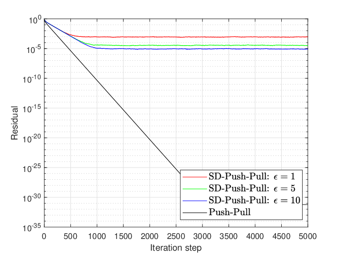
Assume $\epsilon_{i}=\epsilon,\forall i=\{1,2,3,4,5\}$ and $\delta=10$ . To investigate the dependence of the algorithm accuracy with differential privacy level, we compare the performance SD-Push-Pull for three cases: $\epsilon=1,\epsilon=5$ and $\epsilon=10$ , in terms of the normalized residual $\frac{1}{5}\mathbb{E}\Big[\sum\limits_{i=1}^{5}\frac{||x_{i,k}-x^{\star\top}||_{2}^{2}}{||x_{i,0}-x^{\star\top}||_{2}^{2}}\Big]$ . The results are depicted in Fig. 2, which reflect that SD-Push-Pull becomes suboptimal to guarantee differential privacy, and the constant $\epsilon$ determines a tradeoff between the privacy level and the optimization accuracy.

Refer to caption — Fig. 2: Evolutions of the normalized residual under different settings of the privacy level. The expected residual are approximated by averaging over 50 simulation results. Dimension $p=10$ , stepsize $\alpha=0.01$ and penalty parameter $\rho=0.01$ .

VII CONCLUSION AND FUTURE WORK

In this paper, we considered a distributed optimization problem with differential privacy in the scenario where a network is abstracted as an unbalanced directed graph. We proposed a state-decomposition-based differentially private distributed optimization algorithm (SD-Push-Pull). In particular, the state decomposition mechanism was adopted to guarantee the differential privacy of individuals’ sensitive information. In addition, we proved that each agent reach a neighborhood of the optimum in expectation exponentially fast under a constant stepsize policy. Moreover, we showed that the constants $(\epsilon,\delta)$ determine a tradeoff between the privacy level and the optimization accuracy. Finally, a numerical example was provided that demonstrates the effectiveness of SD-Push-Pull. Future work includes improving the accuracy of the optimization and considering the optimization problem with constraints.

VIII APPENDIX

VIII-A Proof of Lemma 9

The three inequalities embedded in (13) come from (9), (10) and (11), repectively.

First inequality: By Lemma 2, Lemma 3, Lemma 6 and Lemma 8, we can obtain from (9) that

		$\displaystyle\mathbb{E}[\|\|\bar{x}_{k+1}-x^{\star\top}\|\|_{2}^{2}\|\mathcal{F}_{k}]$
		$\displaystyle=\mathbb{E}[\|\|\bar{x}_{k}-\eta^{\prime}g_{k}-x^{\star\top}-\eta^{\prime}(h_{k}-g_{k})-\frac{\eta}{n}u^{\top}\mathbf{T}(\mathbf{\tilde{y}}_{k}-v\bar{y}_{k})\|\|_{2}^{2}\|\mathcal{F}_{k}]$
		$\displaystyle+\mathbb{E}[\|\|\frac{\eta^{\prime}}{n}\mathbf{1}_{n}^{\top}\mathbf{\xi}_{k}\|\|_{2}^{2}\|\mathcal{F}_{k}],$
		$\displaystyle\leq\tau_{1}\mathbb{E}[\|\|\bar{x}_{k}-\eta^{\prime}g_{k}-x^{\star\top}\|\|_{2}^{2}\|\mathcal{F}_{k}]+\frac{2\tau_{1}}{\tau_{1}-1}\mathbb{E}[\|\|\eta^{\prime}(h_{k}-g_{k})\|\|_{2}^{2}\|\mathcal{F}_{k}]$
		$\displaystyle+\frac{2\tau_{1}}{\tau_{1}-1}\mathbb{E}[\|\|\frac{\eta}{n}u^{\top}\mathbf{T}(\mathbf{\tilde{y}}_{k}-v\bar{y}_{k})\|\|_{2}^{2}\|\mathcal{F}_{k}]+\frac{2p\eta^{\prime 2}}{n}\bar{\theta}^{2}.$
		$\displaystyle\leq\tau_{1}(1-\eta^{\prime}\mu)^{2}\mathbb{E}[\|\|\bar{x}_{k}-x^{\star\top}\|\|_{2}^{2}\|\mathcal{F}_{k}]+\frac{2\tau_{1}}{\tau_{1}-1}\mathbb{E}[\|\|\eta^{\prime}(h_{k}-g_{k})\|\|_{2}^{2}\|\mathcal{F}_{k}]$
		$\displaystyle+\frac{2\tau_{1}}{\tau_{1}-1}\mathbb{E}[\|\|\frac{\eta}{n}u^{\top}\mathbf{T}(\mathbf{\tilde{y}}_{k}-v\bar{y}_{k})\|\|_{2}^{2}\|\mathcal{F}_{k}]+\frac{2p\eta^{\prime 2}}{n}\bar{\theta}^{2}.$

Taking $\tau_{1}=\frac{1}{1-\eta^{\prime}\mu}$ , we have

		$\displaystyle\mathbb{E}[\|\|\bar{x}_{k+1}-x^{\star\top}\|\|_{2}^{2}\|\mathcal{F}_{k}]$
		$\displaystyle\leq(1-\eta^{\prime}\mu)\mathbb{E}[\|\|\bar{x}_{k}-x^{\star\top}\|\|_{2}^{2}\|\mathcal{F}_{k}]+c_{1}\eta\mathbb{E}[\|\|\mathbf{x}_{k}-\mathbf{1}_{n}{\bar{x}}_{k}\|\|_{2}^{2}\|\mathcal{F}_{k}]$
		$\displaystyle+c_{2}\eta\mathbb{E}[\|\|\mathbf{y}_{k}-v\bar{y}_{k}\|\|_{2}^{2}\|\mathcal{F}_{k}]+c_{3}\eta^{2}\bar{\theta}^{2},$

where

c_{1}=\frac{2u^{\top}\mathbf{T}vL^{2}}{\mu n^{2}},\quad c_{2}=\frac{2||u^{\top}\mathbf{T}||_{2}^{2}}{u^{\top}\mathbf{T}v\mu n},\quad c_{3}=\frac{2p(u^{\top}\mathbf{T}v)^{2}}{n^{3}}.

(39)

Second inequality: By relation (10), Lemma 5, Lemma 6 and Lemma 8, we can obtain

		$\displaystyle\mathbb{E}[\|\|\mathbf{x}_{k+1}-\mathbf{1}_{n}\bar{x}_{k+1}\|\|^{2}_{R}\|\mathcal{F}_{k}]$
		$\displaystyle\leq\tau_{2}\sigma_{R}^{2}\mathbb{E}[\|\|\mathbf{x}_{k}-\mathbf{1}_{n}\bar{x}_{k}\|\|_{R}^{2}\|\mathcal{F}_{k}]+\frac{\tau_{2}\sigma_{R}^{2}\eta^{2}}{\tau_{2}-1}\|\|\mathbf{T}\|\|_{R}^{2}\mathbb{E}[\|\|\mathbf{\tilde{y}}_{k}\|\|_{R}^{2}\|\mathcal{F}_{k}]$
		$\displaystyle\leq\tau_{2}\sigma_{R}^{2}\mathbb{E}[\|\|\mathbf{x}_{k}-\mathbf{1}_{n}\bar{x}_{k}\|\|_{R}^{2}\|\mathcal{F}_{k}]+\frac{2\tau_{2}\sigma_{R}^{2}\eta^{2}}{\tau_{2}-1}\|\|\mathbf{T}v\|\|_{R}^{2}\mathbb{E}[\|\|\bar{y}_{k}\|\|_{R}^{2}\|\mathcal{F}_{k}]$
		$\displaystyle+\frac{2\tau_{2}\sigma_{R}^{2}\eta^{2}}{\tau_{2}-1}\|\|\mathbf{T}\|\|_{R}^{2}\mathbb{E}[\|\|\mathbf{\tilde{y}}_{k}-v\bar{y}_{k}\|\|_{R}^{2}\|\mathcal{F}_{k}].$

In view of Lemma 2,

	$\displaystyle\mathbb{E}[\|\|\bar{y}_{k}\|\|_{2}^{2}\|\mathcal{F}_{k}]\leq\frac{2p\bar{\theta}^{2}}{n}$	$\displaystyle+\frac{2L^{2}}{n}\mathbb{E}[\|\|\mathbf{x}_{k}-\mathbf{1}_{n}\bar{x}_{k}\|\|_{2}^{2}\|\mathcal{F}_{k}]$		(40)
		$\displaystyle+2L^{2}\mathbb{E}[\|\|\bar{x}_{k}-x^{\star\top}\|\|_{2}^{2}\|\mathcal{F}_{k}].$		(40)

Taking $\tau_{2}=\frac{1+\sigma_{R}^{2}}{2\sigma_{R}^{2}}$ , given $1+\sigma_{R}^{2}<2$ , we can obtain

		$\displaystyle\mathbb{E}[\|\|\mathbf{x}_{k+1}-\mathbf{1}_{n}\bar{x}_{k+1}\|\|^{2}_{R}\|\mathcal{F}_{k}]\leq\frac{1+\sigma_{R}^{2}}{2}\mathbb{E}[\|\|\mathbf{x}_{k}-\mathbf{1}_{n}\bar{x}_{k}\|\|_{R}^{2}\|\mathcal{F}_{k}]$
		$\displaystyle+\frac{4\sigma_{R}^{2}\eta^{2}\delta_{R,2}\|\|\mathbf{T}v\|\|_{R}^{2}}{1-\sigma_{R}^{2}}\mathbb{E}[\|\|\bar{y}_{k}\|\|_{2}^{2}\|\mathcal{F}_{k}]$
		$\displaystyle+\frac{4\sigma_{R}^{2}\eta^{2}\delta_{R,C}}{1-\sigma_{R}^{2}}\|\|\mathbf{T}\|\|_{R}^{2}\mathbb{E}[\|\|\mathbf{\tilde{y}}_{k}-v\bar{y}_{k}\|\|_{C}^{2}\|\mathcal{F}_{k}]$
		$\displaystyle\leq c_{4}\eta^{2}\mathbb{E}[\|\|\bar{x}_{k}-x^{\star\top}\|\|_{2}^{2}\|\mathcal{F}_{k}]+(\frac{1+\sigma_{R}^{2}}{2}+c_{5}\eta^{2})$
		$\displaystyle\times\mathbb{E}[\|\|\mathbf{x}_{k}-\mathbf{1}_{n}\bar{x}_{k}\|\|_{R}^{2}\|\mathcal{F}_{k}]+c_{6}\eta^{2}\mathbb{E}[\|\|\mathbf{\tilde{y}}_{k}-v\bar{y}_{k}\|\|_{C}^{2}\|\mathcal{F}_{k}]+c_{7}\eta^{2}\bar{\theta}^{2},$

where

		$\displaystyle c_{4}=\frac{8\sigma_{R}^{2}L^{2}\delta_{R,2}\|\|\mathbf{T}v\|\|_{R}^{2}}{1-\sigma_{R}^{2}},\quad c_{5}=\frac{8\sigma_{R}^{2}L^{2}\delta_{R,2}\|\|\mathbf{T}v\|\|_{R}^{2}}{(1-\sigma_{R}^{2})n},$		(41)
		$\displaystyle c_{6}=\frac{4\sigma_{R}^{2}\delta_{R,C}\|\|\mathbf{T}\|\|_{R}^{2}}{1-\sigma_{R}^{2}},\qquad c_{7}=\frac{8p\sigma_{R}^{2}\delta_{R,2}\|\|\mathbf{T}v\|\|_{R}^{2}}{(1-\sigma_{R}^{2})n}.$		(41)

Third inequality: It follows from (11), Lemma 5, Lemma 6 and Lemma 8 that

		$\displaystyle\mathbb{E}[\|\|\mathbf{\tilde{y}}_{k+1}-v\bar{y}_{k+1}\|\|_{C}^{2}\|\mathcal{F}_{k}]$
		$\displaystyle\leq\frac{1+\sigma_{C}^{2}}{2}\mathbb{E}[\|\|\mathbf{y}_{k}-v\bar{y}_{k}\|\|_{C}^{2}\|\mathcal{F}_{k}]$
		$\displaystyle+\frac{(1+\sigma_{C}^{2})\delta_{C,2}^{2}}{(1-\sigma_{C}^{2})}\|\|\mathbf{I}_{2n}-\frac{v\mathbf{1}_{2n}^{\top}}{n}\|\|_{2}^{2}\mathbb{E}[\|\|\nabla\tilde{F}(\mathbf{x}_{k+1})-\nabla\tilde{F}(\mathbf{x}_{k})\|\|_{2}^{2}\|\mathcal{F}_{k}].$

Next, we bound $\mathbb{E}[||\nabla\tilde{F}(\mathbf{x}_{k+1})-\nabla\tilde{F}(\mathbf{x}_{k})||_{2}^{2}|\mathcal{F}_{k}]$ .

		$\displaystyle\mathbb{E}[\|\|\nabla\tilde{F}(\mathbf{x}_{k+1})-\nabla\tilde{F}(\mathbf{x}_{k})\|\|_{2}^{2}\|\mathcal{F}_{k}]$
		$\displaystyle=\mathbb{E}[\|\|[(\mathbf{\xi}_{k+1}-\mathbf{\xi}_{k})^{\top},(\nabla F(\mathbf{x}_{k+1})-\nabla F(\mathbf{x}_{k}))^{\top}]^{\top}\|\|_{2}^{2}\|\mathcal{F}_{k}]$
		$\displaystyle=\mathbb{E}[\|\|\mathbf{\xi}_{k+1}-\mathbf{\xi}_{k}\|\|_{2}^{2}\|\mathcal{F}_{k}]+\mathbb{E}[\|\|\nabla F(\mathbf{x}_{k+1})-\nabla F(\mathbf{x}_{k})\|\|_{2}^{2}\|\mathcal{F}_{k}]$
		$\displaystyle\leq 4pn\bar{\theta}^{2}+\mathbb{E}[\|\|\nabla F(\mathbf{x}_{k+1})-\nabla F(\mathbf{x}_{k})\|\|_{2}^{2}\|\mathcal{F}_{k}]$

Then, From Assumption 1 and equation (40), we have

		$\displaystyle\mathbb{E}[\|\|\nabla F(\mathbf{x}_{k+1})-\nabla F(\mathbf{x}_{k})\|\|_{2}^{2}\|\mathcal{F}_{k}]$
		$\displaystyle\leq L^{2}\mathbb{E}[\|\|\mathbf{x}_{k+1}-\mathbf{x}_{k}\|\|_{2}^{2}\|\mathcal{F}_{k}]$
		$\displaystyle\leq L^{2}\mathbb{E}[\|\|(\mathbf{R}-\mathbf{I})(\mathbf{x}_{k}-\mathbf{1}_{n}\bar{x}_{k})$
		$\displaystyle-\eta\mathbf{RT}(\mathbf{\tilde{y}}_{k}-v\bar{y}_{k})-\eta\mathbf{RT}v\bar{y}_{k}\|\|_{2}^{2}\|\mathcal{F}_{k}]$
		$\displaystyle\leq 3L^{2}\|\|\mathbf{R}-\mathbf{I}\|\|_{2}^{2}\mathbb{E}[\|\|\mathbf{x}_{k}-\mathbf{1}_{n}\bar{x}_{k}\|\|_{2}^{2}\|\mathcal{F}_{k}]+3L^{2}\eta^{2}\|\|\mathbf{R}\mathbf{T}\|\|_{2}^{2}$
		$\displaystyle\times\mathbb{E}[\|\|\mathbf{\tilde{y}}_{k}-v\bar{y}_{k}\|\|_{2}^{2}\|\mathcal{F}_{k}]+3L^{2}\eta^{2}\|\|\mathbf{R}\mathbf{T}\|\|_{2}^{2}\|\|v\|\|_{2}^{2}\mathbb{E}[\|\|\bar{y}_{k}\|\|_{2}^{2}\|\mathcal{F}_{k}]$

In light of inequality (40), we further have

		$\displaystyle\mathbb{E}[\|\|\nabla F(\mathbf{x}_{k+1})-\nabla F(\mathbf{x}_{k})\|\|_{2}^{2}\|\mathcal{F}_{k}]$
		$\displaystyle\leq(3L^{2}\|\|\mathbf{R}-\mathbf{I}\|\|_{2}^{2}+\frac{6L^{4}\eta^{2}\|\|\mathbf{R}\mathbf{T}\|\|_{2}^{2}\|\|v\|\|_{2}^{2}}{n})\mathbb{E}[\|\|\mathbf{x}_{k}-\mathbf{1}_{n}\bar{x}_{k}\|\|_{2}^{2}\|\mathcal{F}_{k}]$
		$\displaystyle+3L^{2}\eta^{2}\|\|\mathbf{R}\mathbf{T}\|\|_{2}^{2}\mathbb{E}[\|\|\mathbf{\tilde{y}}_{k}-v\bar{y}_{k}\|\|_{2}^{2}\|\mathcal{F}_{k}]+\frac{6L^{2}\eta^{2}\|\|\mathbf{R}\mathbf{T}\|\|_{2}^{2}\|\|v\|\|_{2}^{2}p\bar{\theta}^{2}}{n}$
		$\displaystyle+6L^{4}\eta^{2}\|\|\mathbf{R}\mathbf{T}\|\|_{2}^{2}\|\|v\|\|_{2}^{2}\mathbb{E}[\|\|\bar{x}_{k}-x^{\star\top}\|\|_{2}^{2}\|\mathcal{F}_{k}]$

Thus, given that $\eta<\frac{1}{L}$ , we can obtain

		$\displaystyle\mathbb{E}[\|\|\mathbf{\tilde{y}}_{k+1}-v\bar{y}_{k+1}\|\|_{C}^{2}\|\mathcal{F}_{k}]$
		$\displaystyle\leq c_{8}\eta^{2}\mathbb{E}[\|\|\bar{x}_{k}-x^{\star\top}\|\|_{2}^{2}\|\mathcal{F}_{k}]+c_{9}\mathbb{E}[\|\|\mathbf{x}_{k}-\mathbf{1}_{n}\bar{x}_{k}\|\|_{2}^{2}\|\mathcal{F}_{k}]$
		$\displaystyle+(\frac{1+\sigma_{C}^{2}}{2}+c_{10}\eta^{2})\mathbb{E}[\|\|\mathbf{\tilde{y}}_{k}-v\bar{y}_{k}\|\|_{2}^{2}\|\mathcal{F}_{k}]+c_{11}\bar{\theta}^{2},$

where

		$\displaystyle c_{8}=\frac{12\delta_{C,2}^{2}L^{4}}{(1-\sigma_{C}^{2})}\|\|\mathbf{I}_{2n}-\frac{v\mathbf{1}_{2n}^{\top}}{n}\|\|_{2}^{2}\|\|\mathbf{R}\mathbf{T}\|\|_{2}^{2}\|\|v\|\|_{2}^{2},$		(42)
		$\displaystyle c_{9}=\frac{2\delta_{C,2}^{2}}{(1-\sigma_{C}^{2})}\|\|\mathbf{I}_{2n}-\frac{v\mathbf{1}_{2n}^{\top}}{n}\|\|_{2}^{2}\Big(3L^{2}\|\|\mathbf{R}-\mathbf{I}\|\|_{2}^{2}$
		$\displaystyle+\frac{6L^{2}\|\|\mathbf{R}\mathbf{T}\|\|_{2}^{2}\|\|v\|\|_{2}^{2}}{n}\Big),$
		$\displaystyle c_{10}=\frac{6\delta_{C,2}^{2}L^{2}}{(1-\sigma_{C}^{2})}\|\|\mathbf{I}_{2n}-\frac{v\mathbf{1}_{2n}^{\top}}{n}\|\|_{2}^{2}\|\|\mathbf{R}\mathbf{T}\|\|_{2}^{2},$
		$\displaystyle c_{11}=\frac{12\delta_{C,2}^{2}p}{(1-\sigma_{C}^{2})n}\|\|\mathbf{I}_{2n}-\frac{v\mathbf{1}_{2n}^{\top}}{n}\|\|_{2}^{2}\|\|\mathbf{R}\mathbf{T}\|\|_{2}^{2}\|\|v\|\|_{2}^{2}.$

References

[1] Philipp Braun, Lars Grüne, Christopher M Kellett, Steven R Weller, and Karl Worthmann. A distributed optimization algorithm for the predictive control of smart grids. IEEE Transactions on Automatic Control, 61(12):3898–3911, 2016.
[2] Sean Dougherty and Martin Guay. An extremum-seeking controller for distributed optimization over sensor networks. IEEE Transactions on Automatic Control, 62(2):928–933, 2016.
[3] Rasool Mohebifard and Ali Hajbabaie. Distributed optimization and coordination algorithms for dynamic traffic metering in urban street networks. IEEE Transactions on Intelligent Transportation Systems, 20(5):1930–1941, 2018.
[4] Angelia Nedic and Asuman Ozdaglar. Distributed subgradient methods for multi-agent optimization. IEEE Transactions on Automatic Control, 54(1):48–61, 2009.
[5] Jinming Xu, Shanying Zhu, Yeng Chai Soh, and Lihua Xie. Augmented distributed gradient methods for multi-agent optimization under uncoordinated constant stepsizes. In 2015 54th IEEE Conference on Decision and Control (CDC), pages 2055–2060. IEEE, 2015.
[6] Solmaz S Kia, Bryan Van Scoy, Jorge Cortes, Randy A Freeman, Kevin M Lynch, and Sonia Martinez. Tutorial on dynamic average consensus: The problem, its applications, and the algorithms. IEEE Control Systems Magazine, 39(3):40–72, 2019.
[7] Shi Pu, Wei Shi, Jinming Xu, and Angelia Nedic. Push-pull gradient methods for distributed optimization in networks. IEEE Transactions on Automatic Control, 2020.
[8] Chenguang Xi, Van Sy Mai, Ran Xin, Eyad H Abed, and Usman A Khan. Linear convergence in optimization over directed graphs with row-stochastic matrices. IEEE Transactions on Automatic Control, 63(10):3558–3565, 2018.
[9] Avikarsha Mandal. Privacy preserving consensus-based economic dispatch in smart grid systems. In International Conference on Future Network Systems and Security, pages 98–110. Springer, 2016.
[10] Yongqiang Wang. Privacy-preserving average consensus via state decomposition. IEEE Transactions on Automatic Control, 64(11):4711–4716, 2019.
[11] Chunlei Zhang and Yongqiang Wang. Enabling privacy-preservation in decentralized optimization. IEEE Transactions on Control of Network Systems, 6(2):679–689, 2018.
[12] Yang Lu and Minghui Zhu. Privacy preserving distributed optimization using homomorphic encryption. Automatica, 96:314–325, 2018.
[13] Erfan Nozari, Pavankumar Tallapragada, and Jorge Cortés. Differentially private average consensus: Obstructions, trade-offs, and optimal algorithm design. Automatica, 81:221–231, 2017.
[14] Zhenqi Huang, Sayan Mitra, and Nitin Vaidya. Differentially private distributed optimization. In Proceedings of the 2015 International Conference on Distributed Computing and Networking, pages 1–10, 2015.
[15] Tie Ding, Shanying Zhu, Jianping He, Cailian Chen, and Xinping Guan. Consensus-based distributed optimization in multi-agent systems: Convergence and differential privacy. In Proceedings of the IEEE Conference on Decision and Control (CDC), pages 3409–3414, 2018.
[16] Tie Ding, Shanying Zhu, Jianping He, Cailian Chen, and Xinping Guan. Differentially private distributed optimization via state and direction perturbation in multi-agent systems. IEEE Transactions on Automatic Control, 2021.
[17] Reza Ghabcheloo, António Pascoal, Carlos Silvestre, and Isaac Kaminer. Coordinated path following control of multiple wheeled robots with directed communication links. In Proceedings of the IEEE Conference on Decision and Control, pages 7084–7089, 2005.
[18] Shiping Yang, Sicong Tan, and Jian-Xin Xu. Consensus based approach for economic dispatch problem in a smart grid. IEEE Transactions on Power Systems, 28(4):4416–4426, 2013.
[19] Shuai Mao, Yang Tang, Zi wei Dong, Ke Meng, Zhao Yang Dong, and Feng Qian. A privacy preserving distributed optimization algorithm for economic dispatch over time-varying directed networks. IEEE Transactions on Industrial Informatics, 2020.
[20] Maojiao Ye, Guoqiang Hu, Lihua Xie, and Shengyuan Xu. Differentially private distributed nash equilibrium seeking for aggregative games. IEEE Transactions on Automatic Control, 67(5):2451–2458, 2021.
[21] Cynthia Dwork, Frank McSherry, Kobbi Nissim, and Adam Smith. Calibrating noise to sensitivity in private data analysis. In Theory of cryptography conference, pages 265–284. Springer, 2006.
[22] Shi Pu, Wei Shi, Jinming Xu, and Angelia Nedić. A push-pull gradient method for distributed optimization in networks. In Proceedings of the IEEE Conference on Decision and Control (CDC), pages 3385–3390, 2018.
[23] Angelia Nedic, Alex Olshevsky, and Wei Shi. Achieving geometric convergence for distributed optimization over time-varying graphs. SIAM Journal on Optimization, 27(4):2597–2633, 2017.
[24] Ran Xin and Usman A Khan. A linear algorithm for optimization over directed graphs with geometric convergence. IEEE Control Systems Letters, 2(3):315–320, 2018.
[25] Shi Pu. A robust gradient tracking method for distributed optimization over directed networks. arXiv preprint arXiv:2003.13980, 2020.
[26] Roger A Horn and Charles R Johnson. Matrix analysis. Cambridge university press, 2012.
[27] Guannan Qu and Na Li. Harnessing smoothness to accelerate distributed optimization. IEEE Transactions on Control of Network Systems, 5(3):1245–1260, 2017.
[28] Shi Pu and Angelia Nedić. Distributed stochastic gradient tracking methods. Mathematical Programming, pages 1–49, 2020.

		$\displaystyle\mathbb{E}[\|\|\bar{x}_{k+1}-x^{\star\top}\|\|_{2}^{2}\|\mathcal{F}_{k}]$
		$\displaystyle=\mathbb{E}[\|\|\bar{x}_{k}-\eta^{\prime}g_{k}-x^{\star\top}-\eta^{\prime}(h_{k}-g_{k})-\frac{\eta}{n}u^{\top}\mathbf{T}(\mathbf{\tilde{y}}_{k}-v\bar{y}_{k})\|\|_{2}^{2}\|\mathcal{F}_{k}]$
		$\displaystyle+\mathbb{E}[\|\|\frac{\eta^{\prime}}{n}\mathbf{1}_{n}^{\top}\mathbf{\xi}_{k}\|\|_{2}^{2}\|\mathcal{F}_{k}],$
		$\displaystyle\leq\tau_{1}\mathbb{E}[\|\|\bar{x}_{k}-\eta^{\prime}g_{k}-x^{\star\top}\|\|_{2}^{2}\|\mathcal{F}_{k}]+\frac{2\tau_{1}}{\tau_{1}-1}\mathbb{E}[\|\|\eta^{\prime}(h_{k}-g_{k})\|\|_{2}^{2}\|\mathcal{F}_{k}]$
		$\displaystyle+\frac{2\tau_{1}}{\tau_{1}-1}\mathbb{E}[\|\|\frac{\eta}{n}u^{\top}\mathbf{T}(\mathbf{\tilde{y}}_{k}-v\bar{y}_{k})\|\|_{2}^{2}\|\mathcal{F}_{k}]+\frac{2p\eta^{\prime 2}}{n}\bar{\theta}^{2}.$
		$\displaystyle\leq\tau_{1}(1-\eta^{\prime}\mu)^{2}\mathbb{E}[\|\|\bar{x}_{k}-x^{\star\top}\|\|_{2}^{2}\|\mathcal{F}_{k}]+\frac{2\tau_{1}}{\tau_{1}-1}\mathbb{E}[\|\|\eta^{\prime}(h_{k}-g_{k})\|\|_{2}^{2}\|\mathcal{F}_{k}]$
		$\displaystyle+\frac{2\tau_{1}}{\tau_{1}-1}\mathbb{E}[\|\|\frac{\eta}{n}u^{\top}\mathbf{T}(\mathbf{\tilde{y}}_{k}-v\bar{y}_{k})\|\|_{2}^{2}\|\mathcal{F}_{k}]+\frac{2p\eta^{\prime 2}}{n}\bar{\theta}^{2}.$

		$\displaystyle\mathbb{E}[\|\|\mathbf{x}_{k+1}-\mathbf{1}_{n}\bar{x}_{k+1}\|\|^{2}_{R}\|\mathcal{F}_{k}]$
		$\displaystyle\leq\tau_{2}\sigma_{R}^{2}\mathbb{E}[\|\|\mathbf{x}_{k}-\mathbf{1}_{n}\bar{x}_{k}\|\|_{R}^{2}\|\mathcal{F}_{k}]+\frac{\tau_{2}\sigma_{R}^{2}\eta^{2}}{\tau_{2}-1}\|\|\mathbf{T}\|\|_{R}^{2}\mathbb{E}[\|\|\mathbf{\tilde{y}}_{k}\|\|_{R}^{2}\|\mathcal{F}_{k}]$
		$\displaystyle\leq\tau_{2}\sigma_{R}^{2}\mathbb{E}[\|\|\mathbf{x}_{k}-\mathbf{1}_{n}\bar{x}_{k}\|\|_{R}^{2}\|\mathcal{F}_{k}]+\frac{2\tau_{2}\sigma_{R}^{2}\eta^{2}}{\tau_{2}-1}\|\|\mathbf{T}v\|\|_{R}^{2}\mathbb{E}[\|\|\bar{y}_{k}\|\|_{R}^{2}\|\mathcal{F}_{k}]$
		$\displaystyle+\frac{2\tau_{2}\sigma_{R}^{2}\eta^{2}}{\tau_{2}-1}\|\|\mathbf{T}\|\|_{R}^{2}\mathbb{E}[\|\|\mathbf{\tilde{y}}_{k}-v\bar{y}_{k}\|\|_{R}^{2}\|\mathcal{F}_{k}].$

	$\displaystyle\mathbb{E}[\|\|\bar{y}_{k}\|\|_{2}^{2}\|\mathcal{F}_{k}]\leq\frac{2p\bar{\theta}^{2}}{n}$	$\displaystyle+\frac{2L^{2}}{n}\mathbb{E}[\|\|\mathbf{x}_{k}-\mathbf{1}_{n}\bar{x}_{k}\|\|_{2}^{2}\|\mathcal{F}_{k}]$		(40)
		$\displaystyle+2L^{2}\mathbb{E}[\|\|\bar{x}_{k}-x^{\star\top}\|\|_{2}^{2}\|\mathcal{F}_{k}].$		(40)

		$\displaystyle\mathbb{E}[\|\|\mathbf{x}_{k+1}-\mathbf{1}_{n}\bar{x}_{k+1}\|\|^{2}_{R}\|\mathcal{F}_{k}]\leq\frac{1+\sigma_{R}^{2}}{2}\mathbb{E}[\|\|\mathbf{x}_{k}-\mathbf{1}_{n}\bar{x}_{k}\|\|_{R}^{2}\|\mathcal{F}_{k}]$
		$\displaystyle+\frac{4\sigma_{R}^{2}\eta^{2}\delta_{R,2}\|\|\mathbf{T}v\|\|_{R}^{2}}{1-\sigma_{R}^{2}}\mathbb{E}[\|\|\bar{y}_{k}\|\|_{2}^{2}\|\mathcal{F}_{k}]$
		$\displaystyle+\frac{4\sigma_{R}^{2}\eta^{2}\delta_{R,C}}{1-\sigma_{R}^{2}}\|\|\mathbf{T}\|\|_{R}^{2}\mathbb{E}[\|\|\mathbf{\tilde{y}}_{k}-v\bar{y}_{k}\|\|_{C}^{2}\|\mathcal{F}_{k}]$
		$\displaystyle\leq c_{4}\eta^{2}\mathbb{E}[\|\|\bar{x}_{k}-x^{\star\top}\|\|_{2}^{2}\|\mathcal{F}_{k}]+(\frac{1+\sigma_{R}^{2}}{2}+c_{5}\eta^{2})$
		$\displaystyle\times\mathbb{E}[\|\|\mathbf{x}_{k}-\mathbf{1}_{n}\bar{x}_{k}\|\|_{R}^{2}\|\mathcal{F}_{k}]+c_{6}\eta^{2}\mathbb{E}[\|\|\mathbf{\tilde{y}}_{k}-v\bar{y}_{k}\|\|_{C}^{2}\|\mathcal{F}_{k}]+c_{7}\eta^{2}\bar{\theta}^{2},$

		$\displaystyle\mathbb{E}[\|\|\nabla\tilde{F}(\mathbf{x}_{k+1})-\nabla\tilde{F}(\mathbf{x}_{k})\|\|_{2}^{2}\|\mathcal{F}_{k}]$
		$\displaystyle=\mathbb{E}[\|\|[(\mathbf{\xi}_{k+1}-\mathbf{\xi}_{k})^{\top},(\nabla F(\mathbf{x}_{k+1})-\nabla F(\mathbf{x}_{k}))^{\top}]^{\top}\|\|_{2}^{2}\|\mathcal{F}_{k}]$
		$\displaystyle=\mathbb{E}[\|\|\mathbf{\xi}_{k+1}-\mathbf{\xi}_{k}\|\|_{2}^{2}\|\mathcal{F}_{k}]+\mathbb{E}[\|\|\nabla F(\mathbf{x}_{k+1})-\nabla F(\mathbf{x}_{k})\|\|_{2}^{2}\|\mathcal{F}_{k}]$
		$\displaystyle\leq 4pn\bar{\theta}^{2}+\mathbb{E}[\|\|\nabla F(\mathbf{x}_{k+1})-\nabla F(\mathbf{x}_{k})\|\|_{2}^{2}\|\mathcal{F}_{k}]$