Probing hundreds of individual quantum defects in polycrystalline and amorphous alumina
Abstract
Quantum two-level systems (TLSs) are present in the materials of qubits and are considered defects because they limit qubit coherence. For superconducting qubits, the quintessential Josephson junction barrier is made of amorphous alumina, which hosts TLSs. However, TLSs are not understood generally – either structurally or in atomic composition. In this study, we greatly extend the quantitative data available on TLSs by reporting on the physical dipole moment in two alumina types: polycrystalline and amorphous . To obtain the dipole moments , rather from the less-structural coupling parameter g, we tune individual TLSs with an external electric field to extract the of the TLSs in a cavity QED system. We find a clear difference in the dipole moment distribution from the film types, indicating a difference in TLS structures. A large sample of approximately 400 individual TLSs are analyzed from the polycrystalline film type. Their dipoles along the growth direction have a mean value of 2.60.3 Debye (D) (0.540.06 e) and standard deviation = 1.60.2 D (0.330.03 e). The material distribution fits well to a single Gaussian function. Approximately 200 individual TLSs are analyzed from amorphous films. Both the mean =4.60.5 D (0.96 e) and =2.50.3 D (0.52 e) are larger. Amorphous alumina also has very large , > 8.6 D (1.8 e), in contrast to polycrystalline which has none of this moment. These large moments agree only with oxygen-based TLS models. Based on data and the candidate models (delocalized O and hydrogen-based TLSs), we find polycrystalline alumina has smaller ratio of O-based to H-based TLS than amorphous alumina.
I Introduction
Long coherence times are essential for quantum information processing and this implies high-quality Josephson junctions (JJs) in superconducting qubits Nakamura et al. 1999; Wallraff et al. 2004; Manucharyan et al. 2009; Devoret and Schoelkopf 2013; Yan et al. 2016; Arute et al. 2019. For over a dozen years, quantum tunneling two-level systems (TLSs) have been known to be defects that cause loss and limit coherence of qubits Simmonds et al. 2004; Martinis et al. 2005. In addition, TLSs create telegraphic noise and 1/f noise Burnett et al. 2014; Meißner et al. 2018; Burnett et al. 2019 in superconducting qubits Müller et al. 2015; Klimov et al. 2018; Schlör et al. 2019, semiconducting qubits Connors et al. 2019, and astronomy photon detectors Noroozian et al. 2009; Gao 2008. There are several strategies to improve the qubit coherence time such as material optimization O’Connell et al. 2008; Lock et al. 2019; Chang et al. 2013; Goetz et al. 2016, surface treatments Goetz et al. 2016; Quintana et al. 2014; Grünhaupt et al. 2017, and engineering of the qubit geometry to decrease the participation of TLSs Paik et al. 2011; Wang et al. 2015; Dial et al. 2016.
In the quintessential JJ, an amorphous alumina barrier is grown thermally on the surface of aluminum Nakamura et al. 1999; Wallraff et al. 2004; Devoret and Schoelkopf 2013. Loss tangents of amorphous alumina in JJs O’Connell et al. 2008 and in grown films Deng 2015 are measured to be approximately , much higher than that in crystalline alumina from the sapphire substrates used for qubit fabrication Creedon et al. 2011. Accordingly, amorphous materials are believed to have higher loss than crystalline ones due to additional tunneling degrees of freedom (TLSs) in the former. HBN and other 2D materials are being investigated for JJs Lee et al. 2019; Wang et al. 2018; Shim and Tahan 2014, but an alternative method to improve the JJ barrier uses annealed crystalline alumina Oh et al. 2006; Weides et al. 2011. Crystalline alumina studies show a decrease in both TLS density Oh et al. 2006 and TLS-qubit couplings, , relative to amorphous alumina Weides et al. 2011.
Recent TLS analysis techniques use dc-tuned electric Sarabi et al. 2016; Bilmes et al. 2021; Bilmes et al. 2020; de Graaf et al. 2021 or strain field Lisenfeld et al. 2010; Grabovskij et al. 2012; Brehm et al. 2017 for the observation of individual nanoscale defects. According to the Standard Tunneling Model (STM) Anderson et al. 1972; Phillips 1972, individual TLSs have a dipole moment , transition energy and tunneling energy . Generally, the TLS is described as tunneling charge presumed to be an atom or small group of atoms, though a recent study reports on a possibility of trapped quasiparticles de Graaf et al. 2020. Their identification is a 50 years old mystery Yu and Carruzzo 2021.
TLSs have an ac-coupling to quantum systems,
| (1) |
which is related to dipole moment component along zero-point fluctuation of electric field . However, the most common measurement of does not allow extraction of because is unknown or is not uniform Martinis et al. 2005; Oh et al. 2006; Weides et al. 2011. On the other hand, static dc-tuned measurements allow measurements of individual Sarabi et al. 2016; Bilmes et al. 2021 and dynamically biased experiments extract averaged Khalil et al. 2014. Such dynamical bias can induce Landau-Zener transitions, and recent work shows that a resonator can even exhibit dynamical decoupling using these transitions Matityahu et al. 2019. Recently, voltage bias gates are added above or below the target area to tune TLSs Bilmes et al. 2020; de Graaf et al. 2021. The extractions of dipoles are possible from and extracted position, but the distribution is given as a function of rather than Bilmes et al. 2020. Also, only small samples of were directly extracted in the past: 13 in amorphous alumina Bilmes et al. 2021 and 64 in silicon nitride Sarabi et al. 2016. To the best of our knowledge, a comparison of in two different materials has not been performed in a single study.
In this letter we study individual TLSs in both polycrystalline alumina and amorphous alumina . We follow the circuit schematic of Ref. Sarabi et al. 2016, and we now name it an Electrical-Bridge Quantum-Defect Sensor (EBQuDS). The TLSs were analyzed in films with an approximate thickness of 20 nm. The TLSs in films are relatively stable, and allow us to obtain a large distribution of 394 TLS dipole moments . In films, 189 TLS moments are extracted despite higher TLS noise. Compared to the film, larger averaged dipole and standard deviation are extracted in films and 10% of TLSs have larger dipole than the maximum extracted in . Specific TLS structures were proposed using available information from recent work on density functional theory (DFT) analysis of TLSs in alumina, where both hydrogen Holder et al. 2013; Gordon et al. 2014 and oxygen DuBois et al. 2013; DuBois et al. 2015; Paz et al. 2014 based TLS have been proposed as the interstitial defects. A comparison of the dipole moments for both and film types allows possible TLS origin identification.
II Method

Fabrication starts by growth of Al/alumina/Al trilayers on a 3-inch Si substrate, where the alumina is the material hosting the TLSs. The method prevents substantial hydrogen contamination, but diffusion of hydrogen is also difficult to prevent in standard lithographic processing Van de Walle and Neugebauer 2003. Then, a first BCl3 etch forms a mesa into the top 2 layers, defining 4 equal capacitors (). Next, a second BCl3 etch forms the base-metal including a resonator inductor L and ground plane. Finally, silicon nitride is deposited as a wiring dielectric, vias are etched by SF6, and an Al wiring layer is defined to connect the inductor to the capacitors. This creates the final resonator structure as shown in Fig. 1 (a). Alumina in the dielectric layer is designed to have an approximate thickness = 20 nm and a volume in each capacitor.
The two sample types are grown in separate chambers. The polycrystalline sample has 20 nm thick film deposited by electron-beam evaporation from 99.99% purity pellets with a base pressure of < torr and alumina is sandwiched by two 100 nm thick aluminum films. On the other hand, the film is 14.7 nm thick with x = 1.3 0.1 and is grown by iterating eight rounds of 1 nm Al deposition followed by static oxidation at 9.5 mbar of oxygen at 250 ∘ C as described in ref. Fritz et al. 2019. Given this oxidation condition, no long-range ordered (crystalline) structure was detected from transmission electron microscopy and only 3% unoxidized aluminum was found inside the layer. Transmission electron microscopy shows that the thickness can vary from 10 to 20 nm in some rare cases.
The resonator inductively couples to the transmission line so that a 2-port microwave transmission measurement can be carried out. The applied voltage from room temperature is filtered by an RC filter, 3dB attenuator and a copper powder filter. It generates an dc biased field across each capacitor. The maximum is with which we observe no refrigerator heating, thus no significant leakage current. Two resonators were fabricated per chip with nominally the same capacitors, but with different value inductors, giving resonance frequencies of approximately 5.0 GHz and 4.4 GHz. The resonators were measured at or below 60 mK. A less than 1 probing photon number is used for all the reported data, to allow observation of TLSs near their ground state.
With a known external field , the asymmetry energy is shifted as Sarabi et al. 2016. Therefore, the resultant TLS energy is
| (2) |
The resonator constitutes a circuit QED system with a Jaynes-Cummings model modified for many TLSs. TLSs can be resolved individually by the resonator when the cooperativity Sarabi et al. 2015, where is the TLS decay rate for the strongly coupled TLS, and is the resonator decay rate from external coupling and internal loss. We increase the and cooperativity by reducing , since in our parallel-plate capacitor resonator Martinis et al. 2005.
A single transmission trace is shown in Fig. 1 (b) from a resonator. Within the bandwidth of the resonator, a few fine resonance dips reveal the energies of individual TLSs. However, the TLSs often only couple weakly to the resonator. Therefore, we obtain an approximate intrinsic material loss tangent by using the averaged traces from different voltage biases, yielding an ensemble-averaged . The || component of the result is shown as the solid black curve in Fig. 1 (b). A fit (dashed red curve) to yields and the external (or coupling) quality factor is extracted as . The same procedure performed on gives an intrinsic loss tangent of , which is smaller than that of . is the averaged of and its are distinct with every cooldown unlike (Appendix C). Our loss tangents are similar to alumina with different growth methods, where the loss is measured at Martinis et al. 2005; Stoutimore et al. 2012, Khalil et al. 2013, and Pappas et al. 2011. Below we discuss TLSs measured in both alumina film types using two resonators for each type.
III Results and Discussion

Fig. 2 (a) shows a TLS spectrum example, , as a function of frequency and the dc-field for measured on one of the two resonators during one cool-down. TLS energies exhibit hyperbolic energies versus , as shown in Fig. 2 (a) in agreement with Eq. 2. Similar spectra have been observed and analyzed in a previous study on silicon nitride Sarabi et al. 2016. One can estimate the from the minimum of the TLS energy (), and from the hyperbola – a steeper curvature gives a larger dipole moment. A optimized Monte Carlo fit is performed on each TLS energy to extract of the specific TLS (see Appendix. D). Only well defined TLS energy curves are selected for analysis. Example fits are plotted as blue hyperbolas in Fig. 2 (b).
TLSs change their energies randomly during cool-downs from room temperature. From four different cool-downs, we created different sets of TLSs in the two resonators with one material type. According to the standard TLS distribution Anderson et al. 1972, TLSs have log-uniform tunneling energies such that there are negligible distribution changes for TLS tunneling energies that are only 0.6 GHz different in our two resonator frequencies (see Appendix. E). We therefore combine all the data from different runs in the two resonators to enlarge the sampling number and improve the statistics: a total of 394 TLSs from two resonators are analyzed to form the measured distribution with an average of 3.5 Debye (D) shown in Fig. 2 (c). The accuracy of extraction is limited by the uniformity of thickness of alumina rather than fitting process. A large amounts of individual TLSs allow relatively accurate representation of the TLS moments in .
Though the measured polycrystalline distribution has a mean value of 3.5 D, this is not an intrinsic material property. At a given electric field bias range , TLSs with larger dipole moments have a larger shift in asymmetry energy relative to smaller moments, and this leads to a higher probability of the former moments having their energy minimum within the resonator bandwidth (see Appendix A and Ref Sarabi et al. 2016). The intrinsic material TLS dipole distribution is related to TLS material density (in units of ), and can be calculated from , where is the resonator frequency and is the frequency span of the measurement. The red dashed line in Fig. 2 (c) shows a fit using a maximum likelihood estimation (MLE) method. The fitting function is a modified Gaussian distribution, which is a Gaussian distribution multiplied by . The TLS material density is shown in Fig. 2 (d), where the red line shows a Gaussian function matching the fit parameters in Fig. 2 (c).
From the fit, we find that the polycrystalline material distribution has a fit mean dipole moment of = 2.6 D (=0.54 e) and = 1.6 D (=0.33 e). The computed TLS density is . This computed value of TLS density along with the dipole moments agrees with the measured loss tangent. As a result we used the material units in panel (d) for the distribution .
For amorphous samples or random voids within polycrystals, we expect TLS dipoles to be random in angle (isotropic). For a case of one single dipole magnitude and uniform distribution in , where is the angle of dipole to z-axis, results isotropy. Therefore, is expected to be independent of until the maximum value . As a guide to the eye, an isotropic distribution (random angle) with dipole moment = 4.5 D is shown as a black dashed line in Fig. 2 (d). The positive slope in the observed distribution indicates that we have a departure from isotropic distribution (isotropic TLSs give only non-positive slope). Thus, data in Fig. 2 (d), shows that TLSs can be different than the standard model for TLSs (designated for amorphous samples Anderson et al. 1972; Phillips 1972). The anisotropic angular distribution may be caused by the polycrystalline film texture (crystallite orientation) which influences the TLS orientation.

Fig. 3 (a) shows transmission spectroscopy results for . However, the spectra are not as clear as in due to higher noise in the spectra, despite using the same setup. To improve the TLS signal contrast, the transmission () data is shown after processing, unlike the polycrystalline film data shown earlier. For our first processing step we chose to subtract from , and increase further contrast using the formula . As a second and third processing step, we apply a low-pass filter in the frequency direction and then take the derivative with respect to frequency. The final result is plotted in arbitrary unit (AU) in Fig. 3 (a) and (b) and we added hyperbolic fitting traces (blue lines) to the panel (b).
As we will show in detail below, TLSs within are less stable than those in – the former TLSs show sudden switchings in energy or even become invisible in time within the resonator bandwidth, making it more difficult to identify individual TLSs. This leads to a higher error in the Monte Carlo fit. We also observed energy features that are almost independent of , as indicated by black arrows. They are not expected because all coupled TLSs should be frequency tunable in the device. At -8 kV/m, one hyperbola seems to change slope (as indicated by the start of a blue dashed line), although instead this event may represent a transition in observing two separate TLSs.
Surprisingly, one of them seems to be only partially described by hyperbola in red-dashed curve. Increasing bias voltage at -30 kV/m, this TLS seems to switch from a regular TLS state to an unknown state which has constant transition energy under bias until -19 kV/m, and finally switch back to normal TLS behavior. This indicates an unexpected state near its energy minima , which we believe has not been identified previously.
Unlike the other sample, the amorphous films show most of the hyperbolas from TLSs in the bias range of to (more data in sup). Outside of this range TLSs tracks are seen, but they don’t trace out a smooth hyperbola. Furthermore, we find that the most TLSs do not appear twice after repeating the voltage scanning within the same cool-down. In a small fraction of TLS hyperbola (< 3%) a TLS hyperbola has the same dipole and the minimum in energy is within 1 MHz, such that it is regarded as the same TLS and disregarded in distribution.
In , we identify and analyze a total of 189 TLSs using multiple field sweeps and cool-downs according to the above procedure. The measured distribution with counts and the probability of material distribution are shown in Fig. 3 (c). The extracted shows a broad range in value from 0.5 to 16 D with an average of 6.0 D and the interquartile range (range from the 25th to 75th points) of 3.8 D. Because of the large deviation, we cannot get a reasonable fitting to a Gaussian from the MLE method as shown in yellow lines, which have mean value of 1.6 D and standard deviation of 4.2 D. Instead, we calculate the material average dipole moment for from , using , and the standard deviation in a similar way. From this we find (= 0.96 e) and = 2.50.3 D (= 0.52 e). A Gaussian curve with these parameters are plotted as red dashed line.
The calculated loss from the dipole distribution is which is smaller than reported above. The missing TLS extraction happens in two ways. On one hand, larger TLSs have a higher possibility to interact with other TLSs and their frequencies are prone to switch to other states or diffuse. On the other hand, small TLSs require longer time to acquire TLS hyperbolas and the signal-to-noise ratio is smaller due to smaller coupling to the resonator. As a result, the TLS extraction does not include most of the TLS unlike the extraction in . We estimate the minimum mean moment of amorphous alumina from missing TLSs. We make no claim about anisotropy in this film since the missing TLSs may create one of the peaks in the distribution of (Appendix G).

To decipher the role of TLS-TLS interaction, we next conduct temporal spectroscopes for the two different film types: and . Fig. 4 shows processed traces observed over many hours. This resonant TLS noise is believed to be caused by interactions with thermally excited low-frequency TLSs Klimov et al. 2018; Faoro and Ioffe 2012. As shown in Fig. 4 (a), TLSs biased at 0 V in films near the resonance frequency are relatively stable – their energies drift by less than 2 MHz over tens of hours. On the contrary, TLSs in behave similar to Ref. Klimov et al. 2018. TLSs show irregular drifts of more than 5 MHz, including multiple telegraphic switching events (blue arrows) and abrupt TLS shifts (black arrow). Due to the larger dipole moments observed in , we expect a larger interaction than that in (assuming that the low-frequency thermally activated TLSs are similar to the high frequency ones). The large unstable behaviors shown in the amorphous films occur in a few hours, e.g., a 4 D hyperbola track in data took about 5 hours to obtain.
Comparable results on amorphous alumina exist. One study found in the range of 2.3 -7.4 D, using a few analyzed TLSs Brehm et al. 2017. Other field tuned measurements in a-AlOx, studying the barrier of JJs, detected several moments with = 1.0 - 2.9 D Bilmes et al. 2021. Measurements of the transition dipole moments in a-AlOx of JJs indicate that 6.0 D Martinis et al. 2005 and 4.8 D Shalibo et al. 2010 in two TLS dipoles measured. The existing data on amorphous alumina TLSs seems consistent with our observations, though the growth methods are slightly different.
Finally, we return to comment on the possible origins of TLSs in our alumina from a comparison to recent TLS DFT Holder et al. 2013; Gordon et al. 2014; DuBois et al. 2013; DuBois et al. 2015 and molecular dynamics Paz et al. 2014 simulations on aluminum oxide. Two models related to hydrogen(H) suggest total dipole moment < 3.0 D Holder et al. 2013; Gordon et al. 2014. Holder et al. find that hydrogen aluminum-vacancy TLSs in have = 3.0 D Holder et al. 2013. Separately, Gordon et al. simulated the interstitial hydrogen in at various two oxygen(O) atoms distances where = 2.2 – 2.7 D Gordon et al. 2014. Besides H-based simulations, two models of O-based TLSs suggest > 4.2 D. DuBois et al. studied models of delocalized oxygen atoms with six neighboring aluminum atoms DuBois et al. 2013; DuBois et al. 2015. They found oxygen deficient for x = 1.25 by varying distances between O and Al atoms, with = 4.2 - 6.5 D for TLSs with tunneling energy = 4 GHz DuBois et al. 2013. Additionally, Paz et al. find natural bi-stable structures in amorphous alumina including only Al and O atoms and calculate an average = 4.2 D from 7 TLSs Paz et al. 2014. Although there are difference between theoretical models, they are consistent in that H-TLSs have smaller than O-TLSs.
The has a single peak at approximately = 2.6 D, which can be sourced from H-TLS or two unresolved peaks of both H- and O-TLSs. Although small in statistics, has a wider spread in and two separate peaks. Furthermore, TLSs have 10 % population with > 8.6 D, where = 8.6 D is the maximum in . Using a comparison between two alumina datasets and the fact that O-based TLS is the larger dipole in DFT structures, we find a higher ratio of O-TLSs to H-TLSs in a-AlOx than .
IV Conclusion
In summary, we have extracted the dipole moment of hundreds of individual TLSs in nanoscale-thick films of (polycrystalline) and (amorphous) alumina. We have used an Electrical-Bridge Quantum Defect Sensor (EBQuDS), which we show is suitable to characterize number of TLSs as quantum defects. Analysis of the measured histogram of reveals that polycrystalline alumina fits well to a single Gaussian peak. From the material distribution (algebraically related to the measured one), we obtain that the mean TLS moment of the polycrystalline film is 2.6 D (= 0.54 e) and = 1.6 D (= 0.33 e). Furthermore, the material distribution disagrees with the isotropic model commonly used in amorphous materials, indicative of a preferred texture (orientation) of the polycrystalline grains which host TLSs. On the other hand, we cannot conclude if amorphous alumina dipoles are isotropic or not because of missing TLSs extraction.
The ability to extract an accurate mean puts constraints on its defect type, and allows us to make first comparisons to new microscopic structures used in DFT calculations. The polycrystalline data show one dominant peak, and could be showing dominance of H-TLSs, or unresolved peaks of both H- and O-TLSs in the distribution. We find that has a larger mean = 4.60.5 D, which is consistent with previous amorphous alumina results. In contrast to , the TLSs switch more rapidly, and our distribution in amorphous alumina yields a larger standard deviation (= 2.50.3 D) and two peaks in contrast to one. The moments above 8.6 D (10% of the distribution) are larger than any TLS in polycrystalline alumina and agree only with calculations of delocalized O atoms. Due to this and other amorphous distribution features, we find that the ratio of O- to H-TLSs is higher in amorphous samples than in the polycrystalline ones. Because of its relative simplicity in distribution, alumina seems to be an important material for further JJ-barrier studies.
V Acknowledgements
We acknowledge Lukas Radke, Hannes Rotzinger (both from Physikalisches Institut, Karlsruhe Institute of Technology, Germany) and Martin Weides (James Watt School of Engineering, University of Glasgow, UK) for support of discussions on amorphous alumina sample growth.
Appendix A Material Density and Loss tangent
In this section, we derive the relationship between material TLS density, and the measured histogram, . In the Standard Tunneling Model (STM) Anderson et al. 1972; Phillips 1972, the authors assumes that the density of levels per unit volume and energy, , depends on tunneling energy but is uniform in giving
| (3) |
where is a constant in unit of ). However, the model only considers a single moment || = . In our experiments, we notice the dipole moment in z axis is not uniform and we add dipole direction and magnitude dependence. For a general case, we write
| (4) |
where is a generalized material TLS distribution and is a new constant. However, depends on 3 Cartesian coordinates, and we only have measurement access to one component, . The full investigation of is beyond the scope of this paper, but we assume that is separable in , , and . Therefore, we consider the case
| (5) |
where and is the material density mentioned in the main text. In TLS spectroscopy, is controlled such that , , and can be extracted for individual TLSs and , where is the thickness of dielectric. Next, we change variables to include through Jacobian transformation giving
| (6) |
is the total number of observed TLSs from measurement histogram, ,
| (7) |
where is the center value and is the bin width of the i-th bin. can also be written related to Eq. 5 as
| (8) |
Substituting Eq. 6 into the above equation, we have
| (9) |
Similarly, we consider the i-th bin of and the number of TLSs in this bin
| (10) |
In the case of small enough and , we obtain
| (11) |
or
| (12) |
where is the measurement frequency span. Thus, we prove that is not proportional to measured histogram , but .
Next, we derive the loss tangent, , from TLS histogram. Following Ref. Gao 2008, loss due to TLSs can be described as
| (13) |
where is the permittivity constant, is the Rabi frequency, and () is TLS relaxation (decoherence) time. The derivation of a similar integral has been presented in reference Gao 2008. In the case when is much smaller than 1,
| (14) |
Next, we estimate the loss tangent of . By replacing from Eq. 12, we get
| (15) |
The function is factor of larger than the equation (S6) in Ref. Sarabi et al. 2016. Notice that the loss tangent from the TLS histogram is similar to the bulk resonator loss tangent, , reported in main text. Last, we estimate the material constant in the same film
| (16) |
In contrast to , the loss tangent of amorphous alumina is 3.2(3) which is few times smaller than the measured amorphous alumina loss tangent (=9.8(9)). It is expected because we do not fit those TLSs with uncompleted hyperbola curves.
Appendix B Internal Quality Factor Fitting And Bias Filtering
In this section, we discuss the effect of bias line filtering and TLS noise on resonator data fittings. Filtering noise in the bias line is essential to study the individual TLSs in both film types. We performed a control experiment with additional bias-line noise. We start from a setup where the bias line has only a low-pass copper powder filter and a 12GHz K&L filter. Fig. 5 (a) shows measurements of TLS spectroscopy with low frequency noise and Fig. 5 (b) shows one || at fixed bias. There is no observation of any individual TLS. Surprisingly, the fit gives an internal quality factor, = 1600, which is higher than = 680 reported in the main text. It is believed that without proper noise filtering, the bias voltage noise strongly affects the visibility of the TLSs. The change of TLS frequency due to voltage noise is
| (17) |
In the case of multiple TLSs coupled to a resonator, the transmission rate Sarabi 2014
| (18) |
where is the cavity’s decay rate to the transmission line, is the cavity decay rate to the environment when no TLSs exist, is the cavity resonance, is the coupling strength of each TLS, is the decoherence rate, and is the resonant frequency of the i-th TLS. Inspired by Ref. Brock et al. 2020, we assume that every TLS experiences a Gaussian voltage noise and we rewrite transmission rate as
| (19) |
where and yy The standard deviation, , of the i-th TLS depends on and such that the sensitivity to voltage noise is described as an averaged effect. The enhancement of exterminates the effect of the i-th TLS. A simulation of different is shown in Fig. 6 (a). Two TLSs are coupled to the resonator. The upper TLS in the plot is not affected by voltage noise and the lower TLS in the plot has , , and a random frequency shift with deviation, . Simulations show that the lower TLS has smaller and smaller effect on the resonator while voltage noise (or ) increases. The phenomena of the voltage noise is qualitatively similar to the increasing decoherence of TLS as shown in Fig. 6 (b).

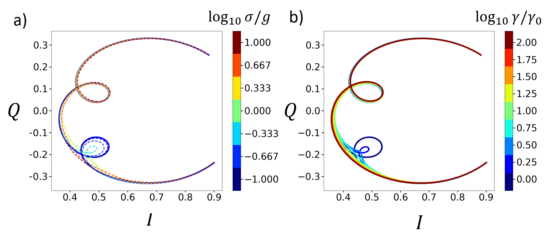
Appendix C Fitting of the averaged of
Due to the low Q (<250) in resonator, the resonator’s transmission data is easily perturbed by frequency-dependent background. For example, there will be (1) spurious modes: existing in the input-output cables, the sample box or on the chip and (2) electrical components: amplifiers, circulators, or attenuation. One obvious result is that the off-resonant part of IQ plot deviates from the circle fitting curve where || is not constant. Thus, we modified the fitting function to better extract resonator’s parameters. We consider the background as multiple low-Q modes, which have no direct coupling with each others and our resonator and the their transmission rate
| (20) |
where and are total quality factor, external quality factor and resonant frequency, respectively. In general, in a small range around resonant frequency , the background can be simplified to , where a and b is a constant. In the case that the of the nearest mode to the measured resonator is in the order of 10 and and each mode separates few hundreds of MHz, can be expanded around to the first order of . As a result, the final fitting function is
| (21) |
Fig. 7 shows two averaged , which are normalized to 1, from two different cooldowns: (a) and (b) are from the dataset of Fig. 12 ; (c) and (d) are from the dataset shown in supplementary sup. To our surprise, the of sample are distinct in different cooldowns and the fits vary from 710 to 1510. We do not understand this variance in amorphous sample and no significant changes for our sample in different cooldowns.
The new averaged of is 1020 for amorphous alumina which is 1.5 times higher than . However, the loss tangent is lower in amorphous alumina can probably because of the below two reasons. First, amorphous alumina can have smaller density of TLSs with higher average dipole moment and lower loss tangent in the end. Second, amorphous alumina has higher voltage noise which eventually reduces the coherent time of TLS and loss tangent. Due to the smaller film thickness and a larger portion of large dipole TLS in , TLSs in suffer from larger voltage noise than those in . One example of extreme cases of high voltage noise is shown in Fig. S1, where we see no TLS and is larger than reported in the main text.

Appendix D Fitting of hyperbolas in DC sweep plot
This section is describing the procedure of fitting TLS dipole for Fig. 2 and 3 in the main text. We search the local minimum (hybridized state) of each from Fig. 2 (a) and apply a Gaussian filter on the 2D plot of local minimum (see Fig. 8 (a) for example). We obtain the initial guess values of , , and for all possible TLS candidates. Due to the complexity of TLS spectrum, TLSs are fit separately in the order of their from the largest to the smallest. The first candidate TLS with the largest is fitted by Monte Carlo method and the result is shown in Fig 8 (b). We assign those local minimum to first TLS and subtract them from Fig. 8 (a) to get Fig. 8 (c). For next TLS, we use the local minimum plot from Fig. 8 (c) and the next fitting will not be affected by the previous TLS result. We repeat the process until all TLSs are fit and discard those TLSs not crossing their minimum energies.

Appendix E TLS histograms in two different resonators
Fig. 9 and Table. 1 show the dipole moment measured in two resonators. The mean are 3.5(1) and 3.6(1), for Res1 with = 4.35 GHz and Res2 with = 4.95 GHz, respectively. Fig 10 shows the dipoles measured in 4 different cooldowns vs either or the external field , where TLSs meet their minimum energies.
Amorphous materials rearrange their atom positions when their temperature is above glass transition temperature (). The thermal cycle to room temperature () is likely not enough. There are chances that TLSs are measured twice in two cooldowns. However, we found the of different cooldowns scatter randomly in the plots (see Fig. 10). Theoretically, TLSs do not change their without reaching . However, we cannot tell if TLSs’ and have changed sufficiently to be considered as new TLSs. But from Fig. 10 (b) and (d), most TLSs ( 85%) have different and in different cooldowns. Whether the thermal cycle is constructing a new set of TLSs is beyond the scope of this paper.

| mean (D) | standard deviation (D) | |
|---|---|---|
| Res1 (4.35 GHz) | 3.55 | 1.47 |
| Res2 (4.95 GHz) | 3.64 | 1.3 |

Appendix F Fitting of TLS density by maximum likelihood estimation
Here, we show the procedure of applying Fisher’s maximum likelihood estimation (MLE) on our statistics. For simplicity, we choose truncated normal distribution as our target function to fit our material density , and
| (22) |
, where is the mean value, is the standard deviation. The normalized constant
| (23) |
depends only on and , where erf(x) is error function defined as
| (24) |
The likelihood function
| (25) |
The necessary conditions for the occurrence of a maximum (or a minimum) are
| (26) |
As mentioned above in Sec. S-I, is not a directly measurement result, but is. Since there is a weighing factor transferring to , we have
| (27) |
A new normalization constant is
| (28) |
and is the total observed TLS.
We also apply a gamma distribution function to fit the data, where
| (29) |
and is a gamma function. The fitting result gives = 5.15 and = 1.72 and mean = 2.99 D. However, we expect there is a distribution > 0 when dipole equals 0 so that gamma distribution is not suitable.
MLE method applied to the amorphous alumina measured histogram does not give the main peak feature adequately in the material distribution . Thus, we do not use MLE to report averaged dipole in the amorphous data, but rather a calculated mean and standard deviation. The calculation method is described in the main text.

Appendix G Estimation of averaged dipole in under TLS frequency noise


Because of the unstable TLS during voltage bias, and resonator noise level, we are prone to measure the larger dipole moments than the smaller ones especially in amorphous sample. Those TLSs without crossing their minimum are not counted in statistics due to the high uncertainty. We show few examples in Fig. 12 (c), where preliminary manual fits are shown in dashed line. A closer look, one can see some other potential small dipole moment TLSs at the edges of the figure.
Here we estimate a case when we miss M-1 out of M small dipole moment by multiplying the small TLS distribution. First, we define the small TLSs as the 10th or 20th percentile, which equals 2.8 and 3.5 Debye respectively. The dipole smaller than the above value are multiplied M times in counts for a new distribution. The resulting new average dipole and ratio of small TLS number to the total number are plotted in Fig. 13. Suppose an extreme case with 8 missing TLS and 2 fitted TLS with < 3.5 D, it means 4 out of 5 are missed. This implies multiple factor M of 5 and the new average is at least 3.3 Debye. This is still larger than = 2.6 Debye in . Now, we turn to the isotropy of dipole orientation. There are missing TLS extractions, especially of those small TLS. The portion of small TLS could be underestimated. As a result, if we add those small back, the material distribution could be monotonic decreasing as expected in the standard model. More studies are needed to understand the small dipole TLSs in amorphous phase.
References
- Nakamura et al. (1999) Y. Nakamura, Y. A. Pashkin, and J. S. Tsai, Coherent control of macroscopic quantum states in a single-cooper-pair box, nature 398, 786 (1999).
- Wallraff et al. (2004) A. Wallraff, D. I. Schuster, A. Blais, L. Frunzio, R.-S. Huang, J. Majer, S. Kumar, S. M. Girvin, and R. J. Schoelkopf, Strong coupling of a single photon to a superconducting qubit using circuit quantum electrodynamics, Nature 431, 162 (2004).
- Manucharyan et al. (2009) V. E. Manucharyan, J. Koch, L. I. Glazman, and M. H. Devoret, Fluxonium: Single cooper-pair circuit free of charge offsets, Science 326, 113 (2009).
- Devoret and Schoelkopf (2013) M. H. Devoret and R. J. Schoelkopf, Superconducting circuits for quantum information: an outlook, Science 339, 1169 (2013).
- Yan et al. (2016) F. Yan, S. Gustavsson, A. Kamal, J. Birenbaum, A. P. Sears, D. Hover, T. J. Gudmundsen, D. Rosenberg, G. Samach, S. Weber, et al., The flux qubit revisited to enhance coherence and reproducibility, Nature communications 7, 1 (2016).
- Arute et al. (2019) F. Arute, K. Arya, R. Babbush, D. Bacon, J. C. Bardin, R. Barends, R. Biswas, S. Boixo, F. G. Brandao, D. A. Buell, et al., Quantum supremacy using a programmable superconducting processor, Nature 574, 505 (2019).
- Simmonds et al. (2004) R. W. Simmonds, K. Lang, D. A. Hite, S. Nam, D. P. Pappas, and J. M. Martinis, Decoherence in josephson phase qubits from junction resonators, Physical Review Letters 93, 077003 (2004).
- Martinis et al. (2005) J. M. Martinis, K. B. Cooper, R. McDermott, M. Steffen, M. Ansmann, K. Osborn, K. Cicak, S. Oh, D. P. Pappas, R. W. Simmonds, et al., Decoherence in josephson qubits from dielectric loss, Physical review letters 95, 210503 (2005).
- Burnett et al. (2014) J. Burnett, L. Faoro, I. Wisby, V. Gurtovoi, A. Chernykh, G. Mikhailov, V. Tulin, R. Shaikhaidarov, V. Antonov, P. Meeson, et al., Evidence for interacting two-level systems from the 1/f noise of a superconducting resonator, Nature communications 5, 1 (2014).
- Meißner et al. (2018) S. M. Meißner, A. Seiler, J. Lisenfeld, A. V. Ustinov, and G. Weiss, Probing individual tunneling fluctuators with coherently controlled tunneling systems, Physical Review B 97, 180505 (2018).
- Burnett et al. (2019) J. J. Burnett, A. Bengtsson, M. Scigliuzzo, D. Niepce, M. Kudra, P. Delsing, and J. Bylander, Decoherence benchmarking of superconducting qubits, npj Quantum Information 5, 1 (2019).
- Müller et al. (2015) C. Müller, J. Lisenfeld, A. Shnirman, and S. Poletto, Interacting two-level defects as sources of fluctuating high-frequency noise in superconducting circuits, Physical Review B 92, 035442 (2015).
- Klimov et al. (2018) P. Klimov, J. Kelly, Z. Chen, M. Neeley, A. Megrant, B. Burkett, R. Barends, K. Arya, B. Chiaro, Y. Chen, et al., Fluctuations of energy-relaxation times in superconducting qubits, Physical review letters 121, 090502 (2018).
- Schlör et al. (2019) S. Schlör, J. Lisenfeld, C. Müller, A. Bilmes, A. Schneider, D. P. Pappas, A. V. Ustinov, and M. Weides, Correlating decoherence in transmon qubits: Low frequency noise by single fluctuators, Physical review letters 123, 190502 (2019).
- Connors et al. (2019) E. J. Connors, J. Nelson, H. Qiao, L. F. Edge, and J. M. Nichol, Low-frequency charge noise in si/sige quantum dots, Physical Review B 100, 165305 (2019).
- Noroozian et al. (2009) O. Noroozian, J. Gao, J. Zmuidzinas, H. G. LeDuc, and B. A. Mazin, Two-level system noise reduction for microwave kinetic inductance detectors, in AIP Conference Proceedings, Vol. 1185 (American Institute of Physics, 2009) pp. 148–151.
- Gao (2008) J. Gao, The physics of superconducting microwave resonators, Ph.D. thesis, California Institute of Technology (2008).
- O’Connell et al. (2008) A. D. O’Connell, M. Ansmann, R. C. Bialczak, M. Hofheinz, N. Katz, E. Lucero, C. McKenney, M. Neeley, H. Wang, E. M. Weig, et al., Microwave dielectric loss at single photon energies and millikelvin temperatures, Applied Physics Letters 92, 112903 (2008).
- Lock et al. (2019) E. H. Lock, P. Xu, T. Kohler, L. Camacho, J. Prestigiacomo, Y. J. Rosen, and K. D. Osborn, Using surface engineering to modulate superconducting coplanar microwave resonator performance, IEEE Transactions on Applied Superconductivity 29, 1 (2019).
- Chang et al. (2013) J. B. Chang, M. R. Vissers, A. D. Córcoles, M. Sandberg, J. Gao, D. W. Abraham, J. M. Chow, J. M. Gambetta, M. Beth Rothwell, G. A. Keefe, et al., Improved superconducting qubit coherence using titanium nitride, Applied Physics Letters 103, 012602 (2013).
- Goetz et al. (2016) J. Goetz, F. Deppe, M. Haeberlein, F. Wulschner, C. W. Zollitsch, S. Meier, M. Fischer, P. Eder, E. Xie, K. G. Fedorov, et al., Loss mechanisms in superconducting thin film microwave resonators, Journal of Applied Physics 119, 015304 (2016).
- Quintana et al. (2014) C. Quintana, A. Megrant, Z. Chen, A. Dunsworth, B. Chiaro, R. Barends, B. Campbell, Y. Chen, I.-C. Hoi, E. Jeffrey, et al., Characterization and reduction of microfabrication-induced decoherence in superconducting quantum circuits, Applied Physics Letters 105, 062601 (2014).
- Grünhaupt et al. (2017) L. Grünhaupt, U. von Lüpke, D. Gusenkova, S. T. Skacel, N. Maleeva, S. Schlör, A. Bilmes, H. Rotzinger, A. V. Ustinov, M. Weides, et al., An argon ion beam milling process for native alox layers enabling coherent superconducting contacts, Applied Physics Letters 111, 072601 (2017).
- Paik et al. (2011) H. Paik, D. Schuster, L. S. Bishop, G. Kirchmair, G. Catelani, A. Sears, B. Johnson, M. Reagor, L. Frunzio, L. Glazman, et al., Observation of high coherence in josephson junction qubits measured in a three-dimensional circuit qed architecture, Physical Review Letters 107, 240501 (2011).
- Wang et al. (2015) C. Wang, C. Axline, Y. Y. Gao, T. Brecht, Y. Chu, L. Frunzio, M. Devoret, and R. J. Schoelkopf, Surface participation and dielectric loss in superconducting qubits, Applied Physics Letters 107, 162601 (2015).
- Dial et al. (2016) O. Dial, D. T. McClure, S. Poletto, G. Keefe, M. B. Rothwell, J. M. Gambetta, D. W. Abraham, J. M. Chow, and M. Steffen, Bulk and surface loss in superconducting transmon qubits, Superconductor Science and Technology 29, 044001 (2016).
- Deng (2015) C. Deng, Fast control and decoherence in superconducting quantum circuits, Ph.D. thesis (2015).
- Creedon et al. (2011) D. L. Creedon, Y. Reshitnyk, W. Farr, J. M. Martinis, T. L. Duty, and M. E. Tobar, High q-factor sapphire whispering gallery mode microwave resonator at single photon energies and millikelvin temperatures, Applied Physics Letters 98, 222903 (2011).
- Lee et al. (2019) K.-H. Lee, S. Chakram, S. E. Kim, F. Mujid, A. Ray, H. Gao, C. Park, Y. Zhong, D. A. Muller, D. I. Schuster, et al., Two-dimensional material tunnel barrier for josephson junctions and superconducting qubits, Nano letters 19, 8287 (2019).
- Wang et al. (2018) J. I.-J. Wang, D. Rodan-Legrain, L. Bretheau, D. L. Campbell, B. Kannan, D. Kim, M. Kjaergaard, P. Krantz, G. O. Samach, F. Yan, et al., Quantum coherent control of a hybrid superconducting circuit made with graphene-based van der waals heterostructures, arXiv preprint arXiv:1809.05215 (2018).
- Shim and Tahan (2014) Y.-P. Shim and C. Tahan, Bottom-up superconducting and josephson junction devices inside a group-iv semiconductor, Nature communications 5, 1 (2014).
- Oh et al. (2006) S. Oh, K. Cicak, J. S. Kline, M. A. Sillanpää, K. D. Osborn, J. D. Whittaker, R. W. Simmonds, and D. P. Pappas, Elimination of two level fluctuators in superconducting quantum bits by an epitaxial tunnel barrier, Physical Review B 74, 100502 (2006).
- Weides et al. (2011) M. P. Weides, J. S. Kline, M. R. Vissers, M. O. Sandberg, D. S. Wisbey, B. R. Johnson, T. A. Ohki, and D. P. Pappas, Coherence in a transmon qubit with epitaxial tunnel junctions, Applied Physics Letters 99, 262502 (2011).
- Sarabi et al. (2016) B. Sarabi, A. N. Ramanayaka, A. L. Burin, F. C. Wellstood, and K. D. Osborn, Projected dipole moments of individual two-level defects extracted using circuit quantum electrodynamics, Physical review letters 116, 167002 (2016).
- Bilmes et al. (2021) A. Bilmes, S. Volosheniuk, J. D. Brehm, A. V. Ustinov, and J. Lisenfeld, Quantum sensors for microscopic tunneling systems, npj Quantum Information 7, 1 (2021).
- Bilmes et al. (2020) A. Bilmes, A. Megrant, P. Klimov, G. Weiss, J. M. Martinis, A. V. Ustinov, and J. Lisenfeld, Resolving the positions of defects in superconducting quantum bits, Scientific reports 10, 1 (2020).
- de Graaf et al. (2021) S. de Graaf, S. Mahashabde, S. Kubatkin, A. Y. Tzalenchuk, and A. Danilov, Quantifying dynamics and interactions of individual spurious low-energy fluctuators in superconducting circuits, Physical Review B 103, 174103 (2021).
- Lisenfeld et al. (2010) J. Lisenfeld, C. Müller, J. H. Cole, P. Bushev, A. Lukashenko, A. Shnirman, and A. V. Ustinov, Measuring the temperature dependence of individual two-level systems by direct coherent control, Physical review letters 105, 230504 (2010).
- Grabovskij et al. (2012) G. J. Grabovskij, T. Peichl, J. Lisenfeld, G. Weiss, and A. V. Ustinov, Strain tuning of individual atomic tunneling systems detected by a superconducting qubit, Science 338, 232 (2012).
- Brehm et al. (2017) J. D. Brehm, A. Bilmes, G. Weiss, A. V. Ustinov, and J. Lisenfeld, Transmission-line resonators for the study of individual two-level tunneling systems, Applied Physics Letters 111, 112601 (2017).
- Anderson et al. (1972) P. W. Anderson, B. Halperin, and C. M. Varma, Anomalous low-temperature thermal properties of glasses and spin glasses, Philosophical Magazine 25, 1 (1972).
- Phillips (1972) W. Phillips, Tunneling states in amorphous solids, Journal of Low Temperature Physics 7, 351 (1972).
- de Graaf et al. (2020) S. de Graaf, L. Faoro, L. Ioffe, S. Mahashabde, J. Burnett, T. Lindström, S. Kubatkin, A. Danilov, and A. Y. Tzalenchuk, Two-level systems in superconducting quantum devices due to trapped quasiparticles, Science Advances 6, eabc5055 (2020).
- Yu and Carruzzo (2021) C. C. Yu and H. M. Carruzzo, Two-level systems and the tunneling model: A critical view, arXiv preprint arXiv:2101.02787 (2021).
- Khalil et al. (2014) M. Khalil, S. Gladchenko, M. Stoutimore, F. Wellstood, A. Burin, and K. Osborn, Landau-zener population control and dipole measurement of a two-level-system bath, Physical Review B 90, 100201 (2014).
- Matityahu et al. (2019) S. Matityahu, H. Schmidt, A. Bilmes, A. Shnirman, G. Weiss, A. V. Ustinov, M. Schechter, and J. Lisenfeld, Dynamical decoupling of quantum two-level systems by coherent multiple landau–zener transitions, npj Quantum Information 5, 1 (2019).
- Holder et al. (2013) A. M. Holder, K. D. Osborn, C. Lobb, and C. B. Musgrave, Bulk and surface tunneling hydrogen defects in alumina, Physical review letters 111, 065901 (2013).
- Gordon et al. (2014) L. Gordon, H. Abu-Farsakh, A. Janotti, and C. G. Van de Walle, Hydrogen bonds in al 2 o 3 as dissipative two-level systems in superconducting qubits, Scientific reports 4, 1 (2014).
- DuBois et al. (2013) T. C. DuBois, M. C. Per, S. P. Russo, and J. H. Cole, Delocalized oxygen as the origin of two-level defects in josephson junctions, Physical review letters 110, 077002 (2013).
- DuBois et al. (2015) T. C. DuBois, S. P. Russo, and J. H. Cole, Atomic delocalization as a microscopic origin of two-level defects in josephson junctions, New Journal of Physics 17, 023017 (2015).
- Paz et al. (2014) A. P. Paz, I. V. Lebedeva, I. V. Tokatly, and A. Rubio, Identification of structural motifs as tunneling two-level systems in amorphous alumina at low temperatures, Physical Review B 90, 224202 (2014).
- Van de Walle and Neugebauer (2003) C. G. Van de Walle and J. Neugebauer, Universal alignment of hydrogen levels in semiconductors, insulators and solutions, Nature 423, 626 (2003).
- Fritz et al. (2019) S. Fritz, L. Radtke, R. Schneider, M. Luysberg, M. Weides, and D. Gerthsen, Structural and nanochemical properties of al o x layers in al/al o x/al-layer systems for josephson junctions, Physical Review Materials 3, 114805 (2019).
- Sarabi et al. (2015) B. Sarabi, A. N. Ramanayaka, A. L. Burin, F. C. Wellstood, and K. D. Osborn, Cavity quantum electrodynamics using a near-resonance two-level system: Emergence of the glauber state, Applied Physics Letters 106, 172601 (2015).
- Stoutimore et al. (2012) M. Stoutimore, M. Khalil, C. Lobb, and K. Osborn, A josephson junction defect spectrometer for measuring two-level systems, Applied Physics Letters 101, 062602 (2012).
- Khalil et al. (2013) M. Khalil, M. Stoutimore, S. Gladchenko, A. Holder, C. Musgrave, A. Kozen, G. Rubloff, Y. Liu, R. Gordon, J. Yum, et al., Evidence for hydrogen two-level systems in atomic layer deposition oxides, Applied Physics Letters 103, 162601 (2013).
- Pappas et al. (2011) D. P. Pappas, M. R. Vissers, D. S. Wisbey, J. S. Kline, and J. Gao, Two level system loss in superconducting microwave resonators, IEEE Transactions on Applied Superconductivity 21, 871 (2011).
- (58) See Supplemental Material at [URL will be inserted by publisher] for [give brief description of material].
- Faoro and Ioffe (2012) L. Faoro and L. B. Ioffe, Internal loss of superconducting resonators induced by interacting two-level systems, Physical review letters 109, 157005 (2012).
- Shalibo et al. (2010) Y. Shalibo, Y. Rofe, D. Shwa, F. Zeides, M. Neeley, J. M. Martinis, and N. Katz, Lifetime and coherence of two-level defects in a josephson junction, Phys. Rev. Lett. 105, 177001 (2010).
- Sarabi (2014) B. Sarabi, Cavity quantum electrodynamics of nanoscale two-level systems, Ph.D. thesis (2014).
- Brock et al. (2020) B. Brock, M. Blencowe, and A. Rimberg, Frequency fluctuations in tunable and nonlinear microwave cavities, Physical Review Applied 14, 054026 (2020).