A Triangle Inequality for Cosine SimilarityThanks: Part of the work on this paper has been supported by Deutsche Forschungsgemeinschaft (DFG), project number 124020371, within the Collaborative Research Center SFB 876 “Providing Information by Resource-Constrained Analysis”, project A2 Affiliation: TU Dortmund University, Dortmund, Germany
Abstract
Similarity search is a fundamental problem for many data analysis techniques. Many efficient search techniques rely on the triangle inequality of metrics, which allows pruning parts of the search space based on transitive bounds on distances. Recently, Cosine similarity has become a popular alternative choice to the standard Euclidean metric, in particular in the context of textual data and neural network embeddings. Unfortunately, Cosine similarity is not metric and does not satisfy the standard triangle inequality. Instead, many search techniques for Cosine rely on approximation techniques such as locality sensitive hashing. In this paper, we derive a triangle inequality for Cosine similarity that is suitable for efficient similarity search with many standard search structures (such as the VP-tree, Cover-tree, and M-tree); show that this bound is tight and discuss fast approximations for it. We hope that this spurs new research on accelerating exact similarity search for cosine similarity, and possible other similarity measures beyond the existing work for distance metrics.
Keywords:
cosine similarity triangle inequality similarity search1 Introduction
Similarity search is a fundamental problem in data science and is used as a building block in many tasks and applications, such as nearest-neighbor classification, clustering, anomaly detection, and of course information retrieval. A wide class of search algorithms requires a metric distance function, i.e., a dissimilarity measure that satisfies the triangle inequality for any . Intuitively, this is the requirement that the direct path from to is the shortest, and any detour over another point is at least as long. Many dissimilarity measures such as the popular Euclidean distance and Manhattan distance satisfy this property, but not all do: for example the squared Euclidean distance (minimized, e.g., by the popular -means clustering algorithm) does not, even on univariate data: but .
The triangle inequality is a central technique in accelerating similarity search because it allows us to compute a bound on a distance without having to compute it exactly if we know and for some object . With trivial rearrangement and relabeling of and , we can also obtain a lower bound: . Given a maximum search radius , if , we can then infer that cannot be part of the search result. This technique is often combined with a search tree, where each subtree is associated with a routing object , and stores the maximum distance for all in the subtree. If , none of the objects in the subtree can be part of the search result, and we can hence skip many candidates at once. This technique can also be extended to -nearest neighbor and priority search, where we can use the minimum possible distance to prioritize or prune candidates.
Metric similarity search indexes using this approach include the ball-tree [13], the metric tree [18] aka. the vantage-point tree [19], the LAESA index [9, 15], the Geometric Near-neighbor Access Tree (GNAT) [3] aka. multi-vantage-point-tree [2], the M-tree [5], the SA-tree [11] and Distal SAT [4], the iDistance index [6], the cover tree [1], the M-index [12], and many more. (Neither the k-d-tree, quad-tree, nor the R-tree belong to this family, these indexes are coordinate-based, and require lower-bounds based on hyperplanes and bounding boxes, respectively.) While they differ in the way they organize the data (e.g., with nested balls in the ball tree, M-tree, and cover tree, by splitting into ball-and-remainder in the VP-tree, or by storing the distances to reference points in LAESA and iDistance), all of these examples rely on the triangle inequality for pruning candidates as central search technique, and should not be used with a distance that does not satisfy this condition, as the search results may otherwise be incomplete (this may, however, be acceptable for certain applications).
In this paper, we introduce a triangle inequality for Cosine similarity that allows lifting most of these techniques from metric distances to Cosine similarity, and we hope that future research will allow extending this to other popular similarity functions.
2 Cosine Distance and Euclidean Distance
Cosine similarity (which we will simply denote as “” in the following) is commonly defined as the Cosine of the angle between two vectors and :
Cosine similarity has some interesting properties that make it a popular choice in certain applications, in particular in text analysis. First of all, it is easy to see that for any , i.e., the similarity is invariant to scaling vectors with a positive scalar. In text analysis, this often is a desirable property as repeating the contents of a document multiple times does not change the information of the document substantially. Formally, Cosine similarity can be seen as being the dot product of normalized vectors. Secondly, the computation of Cosine similarity is fairly efficient for sparse vectors: rather than storing the vectors as a long array of values, most of which are zero, they can be encoded for example as pairs of an index and a value , where only the non-zero pairs are stored and kept in sorted order. The dot product of two such vectors can then be efficiently computed by a merge operation, where only those indexes need to be considered that are in both vectors because in only those terms matter where both and are not zero.
In popular literature, you will often find the claim that Cosine similarity is more suited for high-dimensional data. As we will see below, it cannot be superior to Euclidean distance because of the close relationship of the two, hence this must be considered a myth. Research on intrinsic dimensionality has shown that Cosine similarity is also affected by the distance concentration effect [10] as well as the hubness phenomenon [14], two key aspects of the “curse of dimensionality” [20]. The main difference is that we are usually using the Cosine similarity on sparse data, which has a much lower intrinsic dimensionality than the vector space dimensionality suggests.
Consider the Euclidean distance of two normalized vectors and . By expanding the binomials, we obtain:
| (1) | ||||
| (2) |
where the last step relies on the vectors being normalized to unit length. Hence we have an extremely close relationship between Cosine similarity and (squared) Euclidean distance of the normalized vectors:
| (3) |
While we can also compute Euclidean distance more efficiently for sparse vectors using the scalar product form of Eq. 1, this computation is prone to a numerical problem called “catastrophic cancellation” for small distances (when that can be problematic in clustering (see, e.g., [16, 8]). Hence, working with Cosines directly is preferable when possible, and additional motivation for this work was to work directly with a triangle inequality on the similarities, to avoid this numerical problem (as we will see below, we cannot completely avoid this, unless we can afford to compute many trigonometric functions).
In common literature, the term “Cosine distance” usually refers to a dissimilarity function defined as
| (4) | ||||
| which unfortunately is not a metric, i.e., it does not satisfy the triangle inequality. There are two less common alternatives, namely: | ||||
| (5) | ||||
| (6) | ||||
which are less common (but, e.g., available in ELKI [17]) and which are metric. Eq. 5 directly follows from Eq. 3, while the second one is the angle between the vectors itself (the arc length, not the cosine of the angle), for which we easily obtain the triangle inequality by looking at the arc through , , . We will use these metrics below to obtain a triangle inequality for Cosines.
3 Constructing a Triangle Inequality for Cosine Similarity
Because the triangle inequality is the central rule to avoiding distance computations in many metric search indexes (as well as in many other algorithms), we would like to obtain a triangle inequality for Cosine similarity. Given the close relationship to squared Euclidean distance outlined in the previous section, one obvious approach would be to just use Euclidean distance instead of Cosine. If we know that our data is normalized (which is a best practice when using Cosine similarities), we can make the computation slightly more efficient using Eq. 5, but we wanted to avoid this because (i) computing the square root takes 10–50 CPU cycles (depending on the exact CPU, precision, and input value) and (ii) the subtraction in this equation is prone to catastrophic cancellation when the two vectors are similar, i.e., we may have precision issues when finding the nearest neighbors. Hence, we would like to develop techniques that primarily rely on similarity instead of distance, yet allow a similar pruning to the (very successful) metric search acceleration techniques.
Using Eq. 5 and the triangle inequality of Euclidean distance, we obtain
| (7) | ||||
| which, unfortunately, does not appear to allow much further simplification. In order to remove the square root, we can approximate it using the smaller of the two similarities : | ||||
| (8) | ||||
This is highly efficient to compute, a strict bound to Eq. 7, but unfortunately also a rather loose bound if one of the similarities is high, but the other is not.
Besides the relationship to squared Euclidean distance, there is another way to obtain a metric from Cosine similarity, namely by using the arc length as in Eq. 6 (i.e., using the angle itself, rather than the Cosine of the angle):
| This also yields a metric on the sphere that satisfies the triangle inequality: | ||||
| and, hence, | ||||
| (9) | ||||
| Computationally, the trigonometric functions involved here are even more expensive (60–100 CPU cycles each), hence using this variant directly is not for free. However, this can be further transformed (c.f., angle addition theorems) to the following equivalent triangle inequality for Cosine similarity: | ||||
| (10) | ||||
This triangle inequality is tighter than the one based on Euclidean distance, and hence we can expect better pruning power than using an index for Euclidean distance or (Eq. 5) in a metric index; while the computational cost has been reduced to the low “overhead” of Euclidean distances. Eq. 9 suggests that it is the tightest possible bound we can obtain because it is directly using the angles, rather than the chord length as used by Euclidean distance. This bound yields a very interesting insight: while the triangle inequality for Euclidean distances – and in the arc lengths – was additive, the main term of this equation in the Cosine domain is multiplicative.
We also investigated approximations to further reduce the computation overhead. By approximating the last term using the smaller similarity only, we get
| (11) |
which is a cheap bound, tighter than Eq. 8, but still too loose.
We can also expand and approximate the last term using both the smaller and the larger value :
and hence obtain the inequality
| (12) |
but this approximation is strictly inferior to Eq. 11.
3.1 Opposite Direction
The opposite direction of the triangle inequality is often as important as the first direction. For distances and the angles, it is simply obtained by moving one term to the other side and renaming. It can then be simplified as before
| (13) | ||||
| It is interesting to see that Equations 10 and 13 together imply that | ||||
i.e., a symmetric error bound for .
4 Experiments
| Name | Eq. | Equation |
|---|---|---|
| Euclidean | (7) | |
| Eucl-LB | (8) | |
| Arccos | (9) | |
| Mult | (10) | |
| Mult-LB1 | (11) | |
| Mult-LB2 | (12) |
Table 1 summarizes the six bounds that we compare concerning their suitability for metric indexing. Note that we will not investigate the actual performance in a similarity index here, but plan to do this in future work. Instead, we want to focus on the bounds themselves concerning three properties:
- 1.
how tight the bounds are, i.e., how much pruning power we lose
- 2.
whether we can observe numerical instabilities
- 3.
the differences in the computational effort necessary


4.1 Approximation Quality
In Fig. 1, we plot the resulting lower bound for the similarity given and using the Euclidean-based bound (Eq. 7) in Fig. 1(a) and the Arccos-based bound (Eq. 9) in Fig. 1(b). A striking difference is visible in the negative domain: if and are opposite directions, and and are also opposite, then and must in turn be similar. The Arccos-based bound produces positive bounds here, while the Euclidean-based bound can go down to . But in many cases where we employ Cosine similarity, our data will be restricted to the non-negative domain, so this is likely not an issue, and could maybe be solved with a simple sign check. Upon closer inspection, we can observe that the bounds found by the Arccos-based approach tend to be substantially higher in particular for input similarities around 0.5. Fig. 1(c) visualizes the difference between the two bounds. We can see that the Euclidean bounds are never higher than the Arccos bound, which is unsurprising as the latter is tight, and the first is a proper lower bound. But we can also see that the difference between the two (and hence the pruning power) can be as big as 0.5. This maximum is attained when the input Cosine similarities are 0.5 (i.e., the known angles are ): The Euclidean bound is -1 then, while the Arccos-based bound is 0. In the typical use case of Cosine on non-negative values, both bounds are effectively trivial. However, there still is a substantial difference for larger input similarities. Averaging over a uniform sampled grid of input values, considering only those where both bounds are non-negative, the average Euclidean bound is 0.2447, while the average Arccos-based bound is 0.3121, about 27.5% higher. Hence, using the Arccos-based bound is likely to yield better performance.


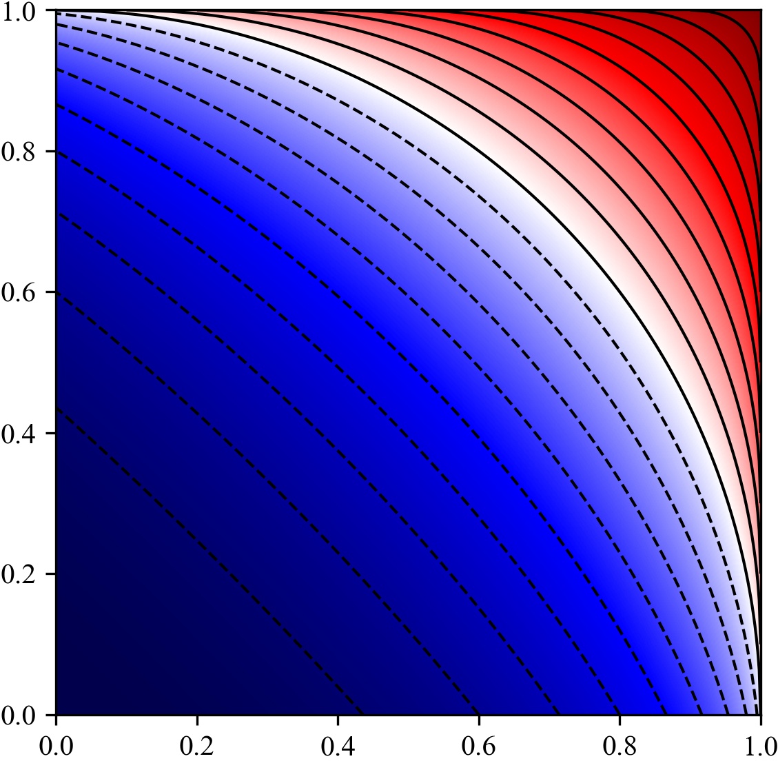

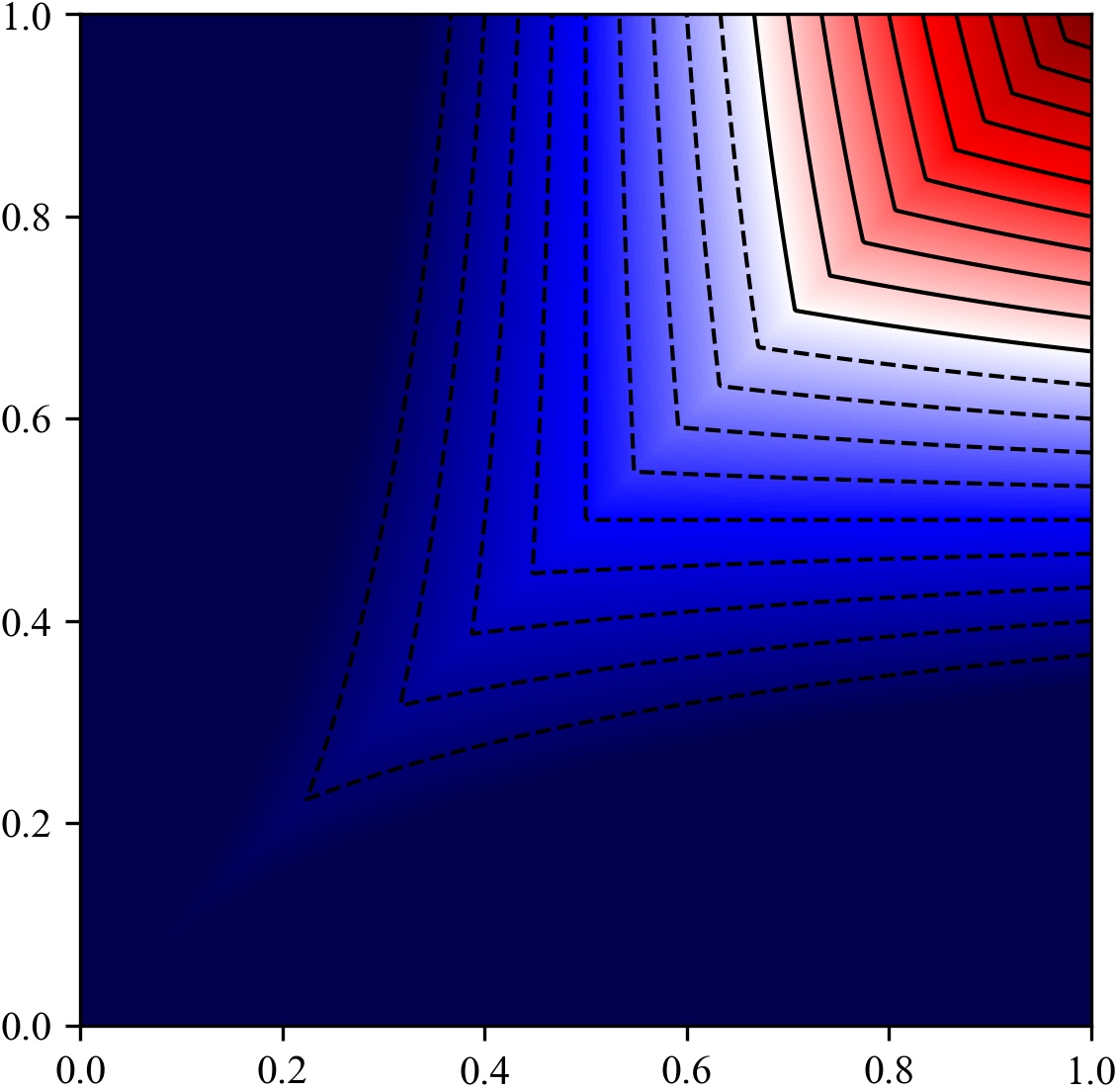
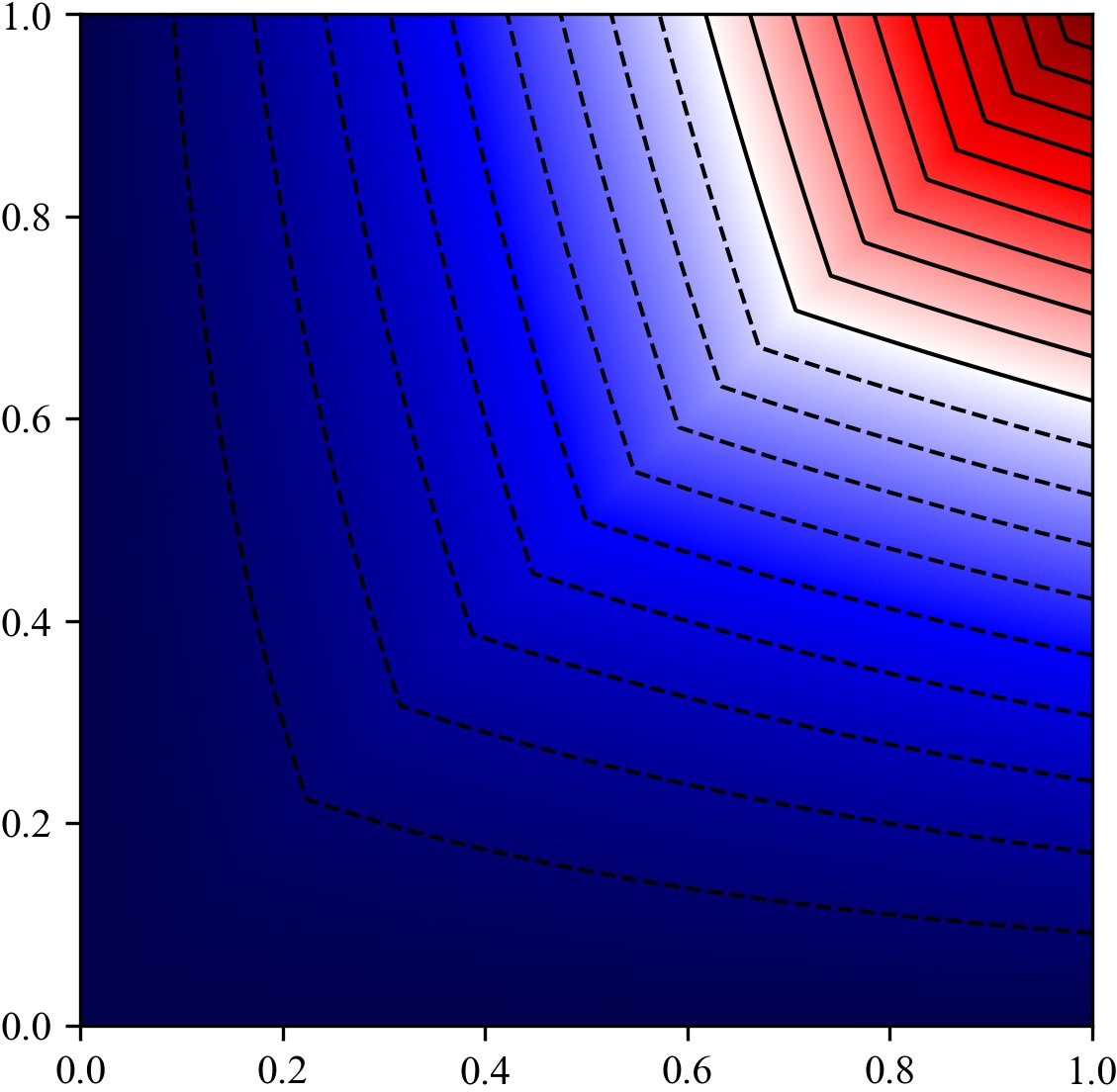
In the following, we focus on the non-negative domain, to improve the readability of the figures. In Fig. 2, we show all six bounds from Table 1. Fig. 2(a) is the Euclidean bound, Fig. 2(b) is the Arccos bound we just saw. Fig. 2(c) is the multiplicative version (Eq. 10), which yields no noticeable difference to the Arccos bound (mathematically, they are equivalent). Fig. 2(d) is the simplified bound derived from Cosine, whereas Fig. 2(e) and Fig. 2(f) are the two bounds derived from the multiplicative version of the Arccos bound. We observe that Mult-LB1 (Fig. 2(f)) is the best of the lower bounds, but also that none of the simplified bounds is a very close approximation to the optimal bounds in the first row. We obtain the following relationship of the presented lower bounds (c.f., Fig. 3):


In Fig. 4 we compare the three simplified bounds (we already compared the Euclidean bound to the tight Arccos bound in Fig. 1(c)). While the Mult-LB1 bound is the best of the simplified bounds, the divergence from the arccos bound can be quite substantial, at least when the two input similarities are not very close. As it can be seen from the isolines in the figures (at steps of 0.1), even if we would consider a bound that is worse by 0.1 or 0.2 acceptable, there remains a fairly large region of relevant inputs (e.g., where one similarity is close to 1.0, the other close to 0.8), where the loss in pruning performance may offset the slightly larger computational cost of using the Mult bound instead.

4.2 Numerical Stability
Mathematically, the Mult bound (Eq. 10) is equivalent to the arccos bound, but more efficient to compute. Given the prior experience with the numerical problem of catastrophic cancellation, we were concerned that this equation might be problematic because of the terms. Fortunately, if , when the problem occurs, the entire square root will become negligible. We have experimented with some alternatives (such as expanding the square root to ), but could not find any benefits. We also compared Mult with the Arccos bound in Fig. 5. While the result appears largely chaotic, the values in this plot are all in the magnitude of , i.e., they are at the expected limit of floating-point precision. Hence, there does not appear to be a numerical instability in this inequality.
4.3 Runtime Experiments
We benchmarked the different equations using Java 11 with double precision floats and the Java Microbenchmarking Harness JMH 1.32.11 1 https://openjdk.java.net/projects/code-tools/jmh/ The experiments were performed on an Intel i7-8650U using a single thread, and with the CPU’s turbo-boost disabled such that the clock rate is stable at 1.9 GHz to reduce measurement noise as well as heat effects. As a baseline, we include a simple add operation to measure the cost of memory access to a pre-generated array of 2 million random numbers. Because trigonometric functions are fairly expensive, we also evaluate the JaFaMa library for fast math as an alternative to the JDK built-ins. JMH is set to perform 5 warmup iterations and 10 measurement iterations of 10 seconds each, to improve the accuracy of our measurements. We try to follow best practices in Java benchmarking (JMH is a well-suited tool for micro-benchmarking in Java), but nevertheless, the results with different programming languages (such as C) can be different due to different compiler optimization, and the usual pitfalls with runtime benchmarks remain [7]. Table 2 gives the results of our experiments. In these experiments, the runtime benefits of the simplified equations are minuscule. Apparently, the CPU can alleviate the latency of the square root to a large extend (e.g., via pipelining), and compared to the memory access cost of the baseline operation, the additional 1.6 nanoseconds will likely not matter for most applications. The benchmark, however, clearly shows the benefit of the “Mult” version over the “Arccos” version, which mathematically is equivalent but differs considerably in run time. While the use of JaFaMa as replacement reduces the runtime considerably, the much simpler “Mult” version still wins hands-down and hence is the version we ultimately recommend using. While “Mult-LB2” is marginally faster, it is also much less accurate and hence useful, as seen in Section 4.1.
| Name | Eq. | Duration | Std.dev. | Accuracy |
| Euclidean | (7) | 10.361 ns | 0.139 ns |
|
| Eucl-LB | (8) | 10.171 ns | 0.132 ns | |
| Arccos | (9) | 610.329 ns | 3.267 ns | |
| Arccos (JaFaMa) | (9) | 58.989 ns | 0.630 ns | |
| Mult (recommended) | (10) | 9.749 ns | 0.096 ns | |
| Mult-variant | 22
2
Eq. 10 expanded using to obtain the variant
|
10.485 ns | 0.022 ns | |
| Mult-LB1 | (11) | 10.313 ns | 0.025 ns | |
| Mult-LB2 | (12) | 8.553 ns | 0.334 ns | |
| Baseline (sum) | 8.186 ns | 0.146 ns | n/a |
5 Conclusions
In this article, we introduce a triangle inequality for Cosine similarity. We study different ways of obtaining a triangle inequality, as well as different attempts at finding an even faster bound. The experiments show that a mathematically equivalent version of the Arccos-based bound is the best trade-off of accuracy (as it has optimal accuracy in our experiments) as well as run-time, where it is only marginally slower than the less accurate alternatives.
Hence, the recommended triangle inequalities for Cosine similarity are:
We can not, however, rule out that there exists a more efficient equation that could be used instead. As this paper shows, there can be more than one version of the same bound that performs very differently due to the functions involved.
We hope to spur new research in the domain of accelerating similarity search with metric indexes, as this equation allows many existing indexes (such as M-trees, VP-trees, cover trees, LAESA, and many more) to be transformed into an efficient index for Cosine similarity. Integrating this equation into algorithms will enable the acceleration of data mining algorithms in various domains, and the use of Cosine similarity directly (without having to transform the similarities into distances first) may both allow simplification as well as optimization of algorithms. Furthermore, we hope that this research can eventually be transferred to other similarity functions besides Cosine similarity. We believe it is a valuable insight that the triangle inequality for Cosine distance contains the product of the existing similarities (but also a non-negligible correction term), whereas the triangle inequality for distance metrics is additive. We wonder if there exists a similarity equivalent of the definition of a metric (i.e., a “simetric”), with similar axioms but for the dual case of similarity functions, but the results above indicate that we will likely not be able to obtain a much more elegant general formulation of a triangle inequality for similarities.
References
- [1] Beygelzimer, A., Kakade, S.M., Langford, J.: Cover trees for nearest neighbor. In: Int. Conf. Machine Learning, ICML. pp. 97–104 (2006). https://doi.org/10.1145/1143844.1143857
- [2] Bozkaya, T., Özsoyoglu, Z.M.: Indexing large metric spaces for similarity search queries. ACM Trans. Database Syst. 24(3), 361–404 (1999). https://doi.org/10.1145/328939.328959
- [3] Brin, S.: Near neighbor search in large metric spaces. In: Dayal, U., Gray, P.M.D., Nishio, S. (eds.) Int. Conf. Very Large Data Bases, VLDB. pp. 574–584. Morgan Kaufmann (1995)
- [4] Chávez, E., Ludueña, V., Reyes, N., Roggero, P.: Faster proximity searching with the distal SAT. In: Int. Conf. Similarity Search and Applications, SISAP. pp. 58–69 (2014). https://doi.org/10.1007/978-3-319-11988-5_6
- [5] Ciaccia, P., Patella, M., Zezula, P.: M-tree: An efficient access method for similarity search in metric spaces. In: Int. Conf. Very Large Data Bases, VLDB. pp. 426–435 (1997)
- [6] Jagadish, H.V., Ooi, B.C., Tan, K., Yu, C., Zhang, R.: idistance: An adaptive b-tree based indexing method for nearest neighbor search. ACM Trans. Database Syst. 30(2), 364–397 (2005). https://doi.org/10.1145/1071610.1071612
- [7] Kriegel, H., Schubert, E., Zimek, A.: The (black) art of runtime evaluation: Are we comparing algorithms or implementations? Knowl. Inf. Syst. 52(2), 341–378 (2017). https://doi.org/10.1007/s10115-016-1004-2
- [8] Lang, A., Schubert, E.: BETULA: numerically stable cf-trees for BIRCH clustering. In: Int. Conf. Similarity Search and Applications, SISAP. pp. 281–296 (2020). https://doi.org/10.1007/978-3-030-60936-8_22
- [9] Micó, L., Oncina, J., Vidal, E.: A new version of the nearest-neighbour approximating and eliminating search algorithm (AESA) with linear preprocessing time and memory requirements. Pattern Recognit. Lett. 15(1), 9–17 (1994). https://doi.org/10.1016/0167-8655(94)90095-7
- [10] Nanopoulos, A., Radovanovic, M., Ivanovic, M.: How does high dimensionality affect collaborative filtering? In: ACM Conf. Recommender Systems, RecSys. pp. 293–296 (2009). https://doi.org/10.1145/1639714.1639771
- [11] Navarro, G.: Searching in metric spaces by spatial approximation. VLDB J. 11(1), 28–46 (2002). https://doi.org/10.1007/s007780200060
- [12] Novak, D., Batko, M., Zezula, P.: Metric index: An efficient and scalable solution for precise and approximate similarity search. Inf. Syst. 36(4), 721–733 (2011). https://doi.org/10.1016/j.is.2010.10.002
- [13] Omohundro, S.M.: Five balltree construction algorithms. Tech. Rep. TR-89-063, International Computer Science Institute (ICSI) (1989)
- [14] Radovanovic, M., Nanopoulos, A., Ivanovic, M.: Nearest neighbors in high-dimensional data: the emergence and influence of hubs. In: Int. Conf. Machine Learning, ICML. pp. 865–872 (2009). https://doi.org/10.1145/1553374.1553485
- [15] Ruiz, G., Santoyo, F., Chávez, E., Figueroa, K., Tellez, E.S.: Extreme pivots for faster metric indexes. In: Int. Conf. Similarity Search and Applications, SISAP. pp. 115–126 (2013). https://doi.org/10.1007/978-3-642-41062-8_12
- [16] Schubert, E., Gertz, M.: Numerically stable parallel computation of (co-)variance. In: Int. Conf. Scientific and Statistical Database Management, SSDBM. pp. 10:1–10:12 (2018). https://doi.org/10.1145/3221269.3223036
- [17] Schubert, E., Zimek, A.: ELKI: A large open-source library for data analysis - ELKI release 0.7.5 ”heidelberg”. CoRR abs/1902.03616 (2019), http://arxiv.org/abs/1902.03616
- [18] Uhlmann, J.K.: Satisfying general proximity/similarity queries with metric trees. Inf. Process. Lett. 40(4), 175–179 (1991). https://doi.org/10.1016/0020-0190(91)90074-R
- [19] Yianilos, P.N.: Data structures and algorithms for nearest neighbor search in general metric spaces. In: ACM/SIGACT-SIAM Symposium on Discrete Algorithms, SODA. pp. 311–321 (1993)
- [20] Zimek, A., Schubert, E., Kriegel, H.: A survey on unsupervised outlier detection in high-dimensional numerical data. Stat. Anal. Data Min. 5(5), 363–387 (2012). https://doi.org/10.1002/sam.11161