Diluting quark flavor hierarchies using dihedral symmetry

The Standard Model (SM) successfully explains the mechanism responsible for the fermion masses but does not justify them. The arbitrariness of the Yukawa couplings makes the SM adaptable to any spectrum of fermion masses and mixings brought in by the experimental measurements. As it happens, the observed quark masses span five orders of magnitudes, with the third generation of quarks being much heavier than the first two. Furthermore, the quark mixings obey the following hierarchical pattern[1]:

$\displaystyle V\approx\begin{pmatrix}1-\lambda^{2}/2&-\lambda&{\mathcal{O}}\left(\lambda^{3}\right)\\ \lambda&1-\lambda^{2}/2&{\mathcal{O}}\left(\lambda^{2}\right)\\ {\mathcal{O}}\left(\lambda^{3}\right)&{\mathcal{O}}\left(\lambda^{2}\right)&1\end{pmatrix}\,,$

(1)

where $\lambda\approx 0.22$ is the Cabibbo mixing parameter and the matrix, $V$, is known as the Cabibbo-Kobayashi-Maskawa (CKM) matrix[2, 3, 4]. Within the ambit of SM, such hierarchies can only originate from some conspiracies within the Yukawa couplings themselves[5]. This is part of the problem that is usually dubbed in the literature as the ‘flavor puzzle’[6, 7, 8]. This aspect of the SM, for decades, has fueled speculations that there might exist a deeper theoretical framework which can offer a more natural insight into the flavor structure. This article presents an extension beyond the SM (BSM) with a $D_{4}$ symmetry, which can make the quark flavor structure appear more instinctive (for other works on flavor models using $D_{4}$ symmetry, see [9, 10, 11, 12, 13, 14, 15, 16, 17]). An essential ingredient of our model is that the primary sources of masses for the third generation of quarks have been disentangled from those for the first two generations of quarks. The hierarchies in the quark masses and mixings are then chiefly attributed to the hierarchies in the vacuum expectation values (VEVs) of the different scalar fields. This allows us to relax the Yukawa hierarchies in the quark sector considerably along with some new and interesting implications for the CKM matrix. We will describe our model in detail in the upcoming sections.

We start by laying out some of the basics of $D_{4}$ symmetry[18]. The discrete group $D_{4}$ has five irreducible representations which we label as $\mathbf{1}_{++}$, $\mathbf{1}_{--}$, $\mathbf{1}_{-+}$, $\mathbf{1}_{+-}$, and $\mathbf{2}$. For the two-dimensional representation of $D_{4}$, we opt to work in a basis in which the generators of $D_{4}$ are given by

$\displaystyle a=\begin{bmatrix}0&-1\\ 1&0\end{bmatrix},\hskip 28.45274ptb=\begin{bmatrix}1&0\\ 0&-1\end{bmatrix}\,,$

(2)

where $a$ is of order 4 and $b$ is of order 2. In this basis, the relevant tensor products in the explicit component form are given by[19]

	$\displaystyle{\begin{bmatrix}x_{1}\\ x_{2}\end{bmatrix}}_{\mathbf{2}}\otimes{\begin{bmatrix}y_{1}\\ y_{2}\end{bmatrix}}_{\mathbf{2}}$	$\displaystyle=$	$\displaystyle{\begin{bmatrix}x_{1}y_{1}+x_{2}y_{2}\end{bmatrix}}_{\mathbf{1}_{++}}\oplus{\begin{bmatrix}x_{1}y_{2}-x_{2}y_{1}\end{bmatrix}}_{\mathbf{1}_{--}}$		(3a)
			$\displaystyle\oplus{\begin{bmatrix}x_{1}y_{2}+x_{2}y_{1}\end{bmatrix}}_{\mathbf{1}_{-+}}\oplus{\begin{bmatrix}x_{1}y_{1}-x_{2}y_{2}\end{bmatrix}}_{\mathbf{1}_{+-}}\,,$
	$\displaystyle\mathbf{1}_{r,s}\otimes\mathbf{1}_{r^{\prime},s^{\prime}}$	$\displaystyle=$	$\displaystyle\mathbf{1}_{r\cdot r^{\prime},s\cdot s^{\prime}}\,.$		(3b)

Now we will specify the $D_{4}$ transformations of the different fields in our model. The $i$-th generation of left-handed quark doublet is denoted by $Q_{iL}\equiv(p_{iL},n_{iL})^{T}$. The right-handed charged quark singlets are denoted by $p_{iR}$ and $n_{iR}$ in the up and down sectors, respectively. We have four scalar doublets in our model, which we symbolize as $\phi_{1}$, $\phi_{2}$, $\phi_{u}$ and $\phi_{d}$. These fields are assumed to transform under the $D_{4}$ symmetry as follows:

	$\displaystyle\textbf{2}:\begin{bmatrix}Q_{1L}\\ Q_{2L}\end{bmatrix}\,,\begin{bmatrix}\phi_{1}\\ \phi_{2}\end{bmatrix}\,,$		(4a)
	$\displaystyle\textbf{1}_{++}:n_{1R}\,,\quad\textbf{1}_{--}:n_{2R}\,,n_{3R}\,,\phi_{u}\,,\quad\textbf{1}_{-+}:p_{2R}\,,p_{3R}\,,\phi_{d}\,,\quad\textbf{1}_{+-}:Q_{3L}\,,p_{1R}\,.$		(4b)

As we will see shortly, because of the above transformations, $\phi_{u}$ and $\phi_{d}$ will couple exclusively to the up and down type quarks respectively, which justifies their labeling. The gauge and $D_{4}$ invariant Yukawa Lagrangians in the up and down quark sectors are then given by

	$\displaystyle-{\mathscr{L}}_{u}$	$\displaystyle=$	$\displaystyle A_{u}(\overline{Q}_{1L}\widetilde{\phi}_{1}-\overline{Q}_{2L}\widetilde{\phi}_{2})p_{1R}+B_{u}(\overline{Q}_{1L}\widetilde{\phi}_{2}+\overline{Q}_{2L}\widetilde{\phi}_{1})p_{2R}+C_{u}(\overline{Q}_{1L}\widetilde{\phi}_{2}+\overline{Q}_{2L}\widetilde{\phi}_{1})p_{3R}$		(5a)
			$\displaystyle+X_{u}\overline{Q}_{3L}\phi_{u}p_{2R}+Y_{u}\overline{Q}_{3L}\phi_{u}p_{3R}\,,$
	$\displaystyle-{\mathscr{L}}_{d}$	$\displaystyle=$	$\displaystyle A_{d}(\overline{Q}_{1L}\phi_{1}+\overline{Q}_{2L}\phi_{2})n_{1R}+B_{d}(\overline{Q}_{1L}\phi_{2}-\overline{Q}_{2L}\phi_{1})n_{2R}+C_{d}(\overline{Q}_{1L}\phi_{2}-\overline{Q}_{2L}\phi_{1})n_{3R}$		(5b)
			$\displaystyle+X_{d}\overline{Q}_{3L}\phi_{d}n_{2R}+Y_{d}\overline{Q}_{3L}\phi_{d}n_{3R}\,,$

where $\widetilde{\phi}_{k}=i\sigma_{2}\phi_{k}^{\star}$ with $\sigma_{2}$ being the second Pauli matrix. For an intuitive understanding of the upcoming results, we will assume the Yukawa parameters to be real. As such, we will not deliberate so much on the complex phase of the CKM matrix. We will treat the phase as an independent parameter which, as we have checked, can be easily accommodated by allowing the Yukawa couplings to be complex. The mass matrices in the up and down sector that transpire from Eq. (5) are

$\displaystyle M_{u}=\begin{pmatrix}A_{u}v_{1}&B_{u}v_{2}&C_{u}v_{2}\\ -A_{u}v_{2}&B_{u}v_{1}&C_{u}v_{1}\\ 0&X_{u}v_{u}&Y_{u}v_{u}\end{pmatrix}\,,\quad M_{d}=\begin{pmatrix}A_{d}v_{1}&B_{d}v_{2}&C_{d}v_{2}\\ A_{d}v_{2}&-B_{d}v_{1}&-C_{d}v_{1}\\ 0&X_{d}v_{d}&Y_{d}v_{d}\end{pmatrix},$

(6)

where $v_{1}$, $v_{2}$, $v_{u}$ and $v_{d}$ represents the VEVs of $\phi_{1}$, $\phi_{2}$, $\phi_{u}$ and $\phi_{d}$ respectively with the total electroweak VEV, $v$, being defined through the relation

$\displaystyle v^{2}=v_{1}^{2}+v_{2}^{2}+v_{u}^{2}+v_{d}^{2}\approx(174~{\rm GeV})^{2}\,.$

(7)

The diagonal mass matrices can then be obtained via the following biunitary transformations:

	$\displaystyle D_{u}$	$\displaystyle=$	$\displaystyle U_{u}M_{u}V_{u}^{\dagger}={\rm diag}(m_{u},~m_{c},~m_{t})\,,$		(8a)
	$\displaystyle D_{d}$	$\displaystyle=$	$\displaystyle U_{d}M_{d}V_{d}^{\dagger}={\rm diag}(m_{d},~m_{s},~m_{b})\,.$		(8b)

Following this convention for the biunitary transformations, the CKM matrix will be given by

$\displaystyle V_{\rm CKM}=U_{u}U_{d}^{\dagger}\,.$

(9)

The matrices $U_{u}$ and $U_{d}$ are obtained by diagonalizing $M_{u}M_{u}^{\dagger}$ and $M_{d}M_{d}^{\dagger}$ respectively, which can be calculated from Eq. (6) as follows:

	$\displaystyle M_{u}M_{u}^{\dagger}$	$\displaystyle=$	$\displaystyle\begin{pmatrix}A_{u}^{2}v_{1}^{2}+(B_{u}^{2}+C_{u}^{2})v_{2}^{2}&(-A_{u}^{2}+B_{u}^{2}+C_{u}^{2})v_{1}v_{2}&(C_{u}Y_{u}+B_{u}X_{u})v_{2}v_{u}\\ (-A_{u}^{2}+B_{u}^{2}+C_{u}^{2})v_{1}v_{2}&(B_{u}^{2}+C_{u}^{2})v_{1}^{2}+A_{u}^{2}v_{2}^{2}&(C_{u}Y_{u}+B_{u}X_{u})v_{1}v_{u}\\ (C_{u}Y_{u}+B_{u}X_{u})v_{2}v_{u}&(C_{u}Y_{u}+B_{u}X_{u})v_{1}v_{u}&(Y_{u}^{2}+{X_{u}}^{2})v_{u}^{2}\end{pmatrix}\,,$		(10a)
	$\displaystyle M_{d}M_{d}^{\dagger}$	$\displaystyle=$	$\displaystyle\begin{pmatrix}A_{d}^{2}v_{1}^{2}+(B_{d}^{2}+C_{d}^{2})v_{2}^{2}&(A_{d}^{2}-B_{d}^{2}-C_{d}^{2})v_{1}v_{2}&(C_{d}Y_{d}+B_{d}X_{d})v_{2}v_{d}\\ (A_{d}^{2}-B_{d}^{2}-C_{d}^{2})v_{1}v_{2}&(B_{d}^{2}+C_{d}^{2})v_{1}^{2}+A_{d}^{2}v_{2}^{2}&-(C_{d}Y_{d}+B_{d}X_{d})v_{1}v_{d}\\ (C_{d}Y_{d}+B_{d}X_{d})v_{2}v_{d}&-(C_{d}Y_{d}+B_{d}X_{d})v_{1}v_{d}&(Y_{d}^{2}+{X_{d}}^{2})v_{d}^{2}\end{pmatrix}\,.$		(10b)

As a matter of fact, both $M_{u}M_{u}^{\dagger}$ and $M_{d}M_{d}^{\dagger}$ can be fully diagonalized analytically by sequentially operating the following matrices:

$\displaystyle O_{\beta}=\begin{pmatrix}\cos\beta&-\sin\beta&0\\ \sin\beta&\cos\beta&0\\ 0&0&1\end{pmatrix}\,,\quad O_{\theta}^{u,d}=\begin{pmatrix}1&0&0\\ 0&\cos\theta_{u,d}&-\sin\theta_{u,d}\\ 0&\sin\theta_{u,d}&\cos\theta_{u,d}\end{pmatrix}\,,$

(11)

where $\tan\beta=v_{2}/v_{1}$ and $\theta_{u,d}$ will be defined shortly. As a first step, we notice that $M_{u}M_{u}^{\dagger}$ and $M_{d}M_{d}^{\dagger}$ can be block diagonalized using $O_{\beta}$ as

	$\displaystyle(M_{u}^{2})_{\rm Block}\equiv O_{\beta}M_{u}M_{u}^{\dagger}O_{\beta}^{\dagger}$	$\displaystyle=$	$\displaystyle\begin{pmatrix}A_{u}^{2}v_{12}^{2}&0&0\\ 0&(B_{u}^{2}+C_{u}^{2})v_{12}^{2}&(C_{u}Y_{u}+B_{u}X_{u})v_{12}v_{u}\\ 0&(C_{u}Y_{u}+B_{u}X_{u})v_{12}v_{u}&(Y_{u}^{2}+{X_{u}}^{2})v_{u}^{2}\end{pmatrix},$		(12a)
	$\displaystyle(M_{d}^{2})_{\rm Block}\equiv O_{\beta}^{\dagger}M_{d}M_{d}^{\dagger}O_{\beta}$	$\displaystyle=$	$\displaystyle\begin{pmatrix}A_{d}^{2}v_{12}^{2}&0&0\\ 0&(B_{d}^{2}+C_{d}^{2})v_{12}^{2}&-(C_{d}Y_{d}+B_{d}X_{d})v_{12}v_{d}\\ 0&-(C_{d}Y_{d}+B_{d}X_{d})v_{12}v_{d}&(Y_{d}^{2}+{X_{d}}^{2})v_{d}^{2}\end{pmatrix},$		(12b)

where, as we will see shortly, $v_{12}^{2}=v_{1}^{2}+v_{2}^{2}$ is the total VEV that is primarily responsible for the light quark masses. Quite clearly, the remaining $2\times 2$ block in the up and down sectors can be diagonalized using $O_{\theta}^{u}$ and $O_{\theta}^{d}$, respectively. This second stage of diagonalization allows us to express $\theta_{u}$ and $\theta_{d}$ in terms of the Yukawa couplings and the VEVs as follows:

	$\displaystyle\tan 2\theta_{u}$	$\displaystyle=$	$\displaystyle\frac{2(C_{u}Y_{u}+B_{u}X_{u})v_{12}v_{u}}{(Y_{u}^{2}+{X_{u}}^{2})v_{u}^{2}-(B_{u}^{2}+C_{u}^{2})v_{12}^{2}}\,,$		(13a)
	$\displaystyle\tan 2\theta_{d}$	$\displaystyle=$	$\displaystyle-\frac{2(C_{d}Y_{d}+B_{d}X_{d})v_{12}v_{d}}{(Y_{d}^{2}+{X_{d}}^{2})v_{d}^{2}-(B_{d}^{2}+C_{d}^{2})v_{12}^{2}}\,.$		(13b)

Thus, the full diagonalization in the up and down sectors can be expressed as

	$\displaystyle D_{u}^{2}=O_{\theta}^{u}O_{\beta}(M_{u}M_{u}^{\dagger})O_{\beta}^{\dagger}{O_{\theta}^{u}}^{\dagger}$	$\displaystyle\equiv$	$\displaystyle{\rm diag}(m_{u}^{2},m_{c}^{2},m_{t}^{2})\,,$		(14a)
	$\displaystyle D_{d}^{2}=O_{\theta}^{d}O_{\beta}^{\dagger}(M_{d}M_{d}^{\dagger})O_{\beta}{O_{\theta}^{d}}^{\dagger}$	$\displaystyle\equiv$	$\displaystyle{\rm diag}(m_{d}^{2},m_{s}^{2},m_{b}^{2})\,.$		(14b)

Following our convention in Eq. (8), the matrices $U_{u}$ and $U_{d}$ can be extracted as follows:

$\displaystyle U_{u}=O_{\theta}^{u}O_{\beta}\,,\qquad U_{d}=O_{\theta}^{d}O_{\beta}^{\dagger}\,.$

(15)

Thus from Eq. (9), the CKM matrix is obtained as

$\displaystyle V_{\rm CKM}=\begin{pmatrix}\cos 2\beta&-\cos\theta_{d}\sin 2\beta&-\sin 2\beta\sin\theta_{d}\\ \cos\theta_{u}\sin 2\beta&\cos 2\beta\cos\theta_{d}\cos\theta_{u}+\sin\theta_{d}\sin\theta_{u}&\cos 2\beta\cos\theta_{u}\sin\theta_{d}-\cos\theta_{d}\sin\theta_{u}\\ \sin 2\beta\sin\theta_{u}&-\cos\theta_{u}\sin\theta_{d}+\cos 2\beta\cos\theta_{d}\sin\theta_{u}&\cos\theta_{d}\cos\theta_{u}+\cos 2\beta\sin\theta_{d}\sin\theta_{u}\end{pmatrix}.$

(16)

To make the connection between Eqs. (16) and (1) apparent, we assume that $v_{12}$ is responsible for the masses of the first two generations of quarks whereas $v_{u}$ and $v_{d}$ primarily contribute to the third generation masses in the up and down sector, respectively. Therefore, it is quite natural to expect $v_{12}\ll v_{u,d}$. From Eq. (12) we identify the first generation quark masses as

$\displaystyle m_{u}^{2}=A_{u}^{2}v_{12}^{2}\,,\qquad m_{d}^{2}=A_{d}^{2}v_{12}^{2}\,.$

(17)

Furthermore, using the VEV hierarchy $v_{u,d}\gg v_{12}$ we can approximate Eq. (13) as

	$\displaystyle\theta_{u}$	$\displaystyle\approx$	$\displaystyle\frac{(C_{u}Y_{u}+B_{u}X_{u})}{(Y_{u}^{2}+{X_{u}}^{2})}\frac{v_{12}}{v_{u}}\approx{\mathcal{O}}\left(\frac{v_{12}}{v_{u}}\right)\,,$		(18a)
	$\displaystyle\theta_{d}$	$\displaystyle\approx$	$\displaystyle-\frac{(C_{d}Y_{d}+B_{d}X_{d})}{(Y_{d}^{2}+{X_{d}}^{2})}\frac{v_{12}}{v_{d}}\approx{\mathcal{O}}\left(\frac{v_{12}}{v_{d}}\right)\,,$		(18b)

where we are implicitly assuming that the involved Yukawa couplings have similar orders of magnitude. It is also quite reasonable to take $v_{12}\sim{\mathcal{O}}\left(1~{\rm GeV}\right)$ and $v_{u,d}\sim{\mathcal{O}}\left(100~{\rm GeV}\right)$ so that the ratio $v_{12}/v_{u,d}$ comes out to be ${\mathcal{O}}\left(\lambda^{2}\right)$. Therefore, from Eq. (18) we conclude

$\displaystyle\sin\theta_{u,d}\approx{\mathcal{O}}\left(\lambda^{2}\right)\,,\qquad\cos\theta_{u,d}\approx{\mathcal{O}}\left(1\right)\,.$

(19)

Moreover, if we identify $\sin 2\beta$ as the Cabibbo mixing, namely,

$\displaystyle\sin 2\beta=\lambda\,,$

(20)

then Eq. (16) resembles exactly to Eq. (1). All these intuitive results will be validated later by providing explicit numerical benchmarks.

Given the structure of the CKM matrix predicted by the model as a function of $\beta$ and $\theta_{u,d}$, shown in Eq. (16), it is possible to extract the quark mixing angles by comparing the CKM matrix with the standard parametrization[20]. This, in turn, allows us to find the following best-fit values of $\beta$ and $\theta_{u,d}$ such that the quark mixing angles are compatible with the observed values[21]:

$$\sin 2\beta\approx 0.2265\,,\qquad\theta_{u}\approx\pm 0.025,\qquad\theta_{d}\approx\mp 0.016.$$

(21)

As expected, the above values for $\sin 2\beta$ and $\theta_{u,d}$ conform well to our intuitive expectations of Eqs. (19) and (20). Fixing $\sin 2\beta$ at its best-fit value, in Fig. 1 we display the region in $\sin\theta_{u}$- $\sin\theta_{d}$ plane allowed by the experimental uncertainties.

For the sake of completeness, we also calculate the mass eigenvalues for the second and third generation of quarks by diagonalizing the $2\times 2$ submatrices in Eq. (12). In the up quark sector, we can compare the traces to write

$\displaystyle m_{c}^{2}+m_{t}^{2}=(B_{u}^{2}+C_{u}^{2})v_{12}^{2}+(Y_{u}^{2}+{X_{u}}^{2})v_{u}^{2}\,.$

(22)

Keeping in mind the hierarchies, $v_{u}\gg v_{12}$ and $m_{t}\gg m_{c}$, the above relation can be approximated to express the top quark mass as

$\displaystyle m_{t}^{2}\approx(Y_{u}^{2}+{X_{u}}^{2})v_{u}^{2}\,.$

(23)

Again, from the determinant of the $2\times 2$ block in Eq. (12a), we may write

$\displaystyle m_{c}^{2}m_{t}^{2}=(B_{u}Y_{u}-C_{u}X_{u})^{2}v_{12}^{2}v_{u}^{2}\,.$

(24)

Using the expression for $m_{t}$ from Eq. (23), we can extract the charm quark mass as

$\displaystyle m_{c}^{2}\approx\frac{(B_{u}Y_{u}-C_{u}X_{u})^{2}}{(Y_{u}^{2}+{X_{u}}^{2})}v_{12}^{2}\,.$

(25)

Following the same steps in the down sector, we can obtain

	$\displaystyle m_{s}^{2}$	$\displaystyle\approx$	$\displaystyle\frac{(B_{d}Y_{d}-C_{d}X_{d})^{2}}{(Y_{d}^{2}+{X_{d}}^{2})}v_{12}^{2}\,,$		(26)
	$\displaystyle m_{b}^{2}$	$\displaystyle\approx$	$\displaystyle(Y_{d}^{2}+{X_{d}}^{2})v_{d}^{2}\,.$		(27)

At this point, we wish to emphasize that, assuming the Yukawas couplings to be similar for a particular sector, an obvious outcome of our model is

$\displaystyle\frac{m_{c}}{m_{t}}\approx\frac{v_{12}}{v_{u}}\sim{\mathcal{O}}\left(\lambda^{2}\right)\,,\qquad\frac{m_{s}}{m_{b}}\approx\frac{v_{12}}{v_{d}}\sim{\mathcal{O}}\left(\lambda^{2}\right)\,,$

(28)

which agrees with the observations.

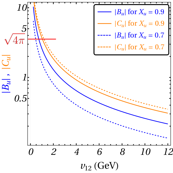
From Eqs. (23) and (25), we see that the third and second generation masses are controlled by $v_{u}$ and $v_{12}$, respectively. We can wonder how perturbativity may affect the model at hand, since $m_{t}\approx{\mathcal{O}}\left(v_{u}\right)$ and $m_{c}\approx{\mathcal{O}}\left(v_{12}\right)$ already[22]. Fig. 2 illustrates how arbitrarily low values of $v_{12}$ may jeopardize the perturbativity of the theory. By choosing $v_{u}=150$ GeV, and two example values for $X_{u}=0.7$ and $0.9$, we can see from Fig. 2 that to have $B_{u}$ and $C_{u}$ in the perturbative regime, we should have $v_{12}\geq\mathcal{O}(1~\text{GeV})$.

Finally, to provide explicit justification to these intuitive expectations, we consider the following benchmark

$$\begin{matrix}v_{12}={2~{\rm GeV}},&v_{u}={150~{\rm GeV}},&v_{d}\approx{88~{\rm GeV}},&&\\ A_{u}\approx 1.08\!\!\times\!\!10^{-3},&B_{u}\approx 1.69,&C_{u}\approx 1.50,&X_{u}\approx 1.04,&Y_{u}\approx 0.49,\\ A_{d}\approx 2.34\!\!\times\!\!10^{-3},&B_{d}\approx 3.65\!\!\times\!\!10^{-2},&C_{d}\approx 4.41\!\!\times\!\!10^{-2},&X_{d}\approx 4.73\!\!\times\!\!10^{-2},&Y_{d}\approx-3.20\!\!\times\!\!10^{-3},\end{matrix}$$

(29)

which results in the following values of the quark masses and mixing angles

	$\displaystyle m_{u}={2.2~{\rm MeV}}\,,\qquad m_{c}={1.27~{\rm GeV}}\,,\qquad m_{t}={173~{\rm GeV}}\,,$		(30a)
	$\displaystyle m_{d}={4.7~{\rm MeV}}\,,\qquad m_{s}={0.093~{\rm GeV}}\,,\qquad m_{b}={4.18~{\rm GeV}}$		(30b)
	$\displaystyle\sin\theta_{12}=0.2265\,,\qquad\sin\theta_{13}=0.0036\,,\qquad\sin\theta_{23}=0.041\,,$		(30c)

which are in agreement with the corresponding observations[21].

In passing, let us highlight the most notable outcomes of our model:

• •

  The hierarchy of the Yukawa couplings is diluted by two orders of magnitude, at least. Recall that, in the SM, $m_{t}=174$ GeV and $m_{u,d}\sim{\mathcal{O}}\left(10^{-3}~\rm GeV\right)$ imply that the quark Yukawa couplings span five orders of magnitudes. We dampen this problem by assuming that the first two generations of quarks receive their masses from $v_{12}$ which is of ${\mathcal{O}}\left(1~{\rm GeV}\right)$. This means, the first generation Yukawas are, at worst, of ${\mathcal{O}}\left(10^{-3}\right)$ whereas the second generation Yukawas can be of ${\mathcal{O}}\left(1\right)$. This feature is quite evident from the benchmark values given in Eq. (29).

• •

  We have introduced $\phi_{u,d}$ dedicated for masses of the third generation of quarks. Quite naturally, we expect, $v_{u,d}\sim{\mathcal{O}}\left(100~{\rm GeV}\right)$ so that the top-Yukawa is of ${\mathcal{O}}\left(1\right)$. Thus, we should have the ratio $v_{12}/v_{u,d}\sim{\mathcal{O}}\left(\lambda^{2}\right)$. It is very interesting to note that, this automatically conforms to $m_{2}/m_{3}\approx v_{12}/v_{u,d}\sim{\mathcal{O}}\left(\lambda^{2}\right)$ where $m_{k}$ is the mass for the $k$-th generation of quark. Quite clearly, this is a natural upshot of our model.

• •

  We have connected the quark mixings with the dynamics of the scalar sector. We have shown that the Cabibbo part of the quark-mixing stems purely from the ratio $v_{2}/v_{1}$ (see Eq. (20)). The smallness of the off-Cabibbo elements of the CKM matrix is further connected to the VEV hierarchy $v_{12}\ll v_{u,d}$. In other way, we are suggesting that the fact that the third generation of quarks are much heavier than the first two generations, is intimately connected to the smallness of the off-Cabibbo elements.

Finally, our current model is not just all about aesthetics, it will have other observable consequences too. The fact that the Yukawa Lagrangian of our model contains fewer parameters than that of the SM comes at the cost of making the scalar potential substantially more involved containing four scalar doublets. This means that the Higgs boson observed at the LHC is not the only fundamental scalar in nature, it is just the first one in series of many others to follow. The physical Higgs bosons will emerge from mixings among the four scalar doublets. Expanding the scalar doublets as

$\displaystyle\phi_{k}=\begin{pmatrix}\varphi_{k}^{+}\\ v_{k}+(h_{k}+iz_{k})/\sqrt{2}\end{pmatrix}\,,\qquad k=1,2,u,d,$

(31)

after the spontaneous symmetry breaking, the SM-like Higgs boson, $h$, can be extracted as follows[23]:

$\displaystyle h=\frac{1}{v}(v_{1}h_{1}+v_{2}h_{2}+v_{u}h_{u}+v_{d}h_{d})\,.$

(32)

This particular linear combination of the component fields will mimic the SM Higgs in its tree-level couplings and will not induce flavor changing neutral currents (FCNCs) at the tree-level. However, the other physical neutral scalars, in general, will possess tree-level FCNCs which means they have to be quite heavy to evade the experimental constraints. To have some intuitions on the FCNC couplings, we analyze the matrices, $N_{d}^{1,2,d}$, which control them in the down sector. Below, we show approximate expressions for these matrices:

	$\displaystyle N_{d}^{1}$	$\displaystyle\approx$	$\displaystyle\frac{1}{\sqrt{2}v_{12}}\begin{pmatrix}m_{d}\cos\beta&-m_{s}\sin\beta&m_{b}\theta_{d}\sin\beta\\ -m_{d}\sin_{\beta}&-m_{s}\cos\beta&m_{b}\theta_{d}\cos\beta\\ -m_{d}\theta_{d}\sin\beta&-m_{s}\theta_{d}\cos\beta&m_{b}\theta_{d}^{2}\cos\beta\end{pmatrix},$		(33a)
	$\displaystyle N_{d}^{2}$	$\displaystyle\approx$	$\displaystyle\frac{1}{\sqrt{2}v_{12}}\begin{pmatrix}m_{d}\sin\beta&m_{s}\cos\beta&-m_{b}\theta_{d}\cos\beta\\ m_{d}\cos\beta&-m_{s}\sin\beta&m_{b}\theta_{d}\sin\beta\\ m_{b}\theta_{d}\cos\beta&-m_{s}\theta_{d}\sin\beta&m_{b}\theta_{d}^{2}\sin\beta\end{pmatrix},$		(33b)
	$\displaystyle N_{d}^{d}$	$\displaystyle\approx$	$\displaystyle\frac{1}{\sqrt{2}v_{d}}\begin{pmatrix}0&0&0\\ 0&0&-m_{b}\theta_{d}\\ 0&0&m_{b}\end{pmatrix}.$		(33c)

From the above expressions, we note that the magnitude of the largest off-diagonal element, for our chosen benchmarks of Eqs. (21) and (29), is $0.033$, which is quite small. On top of this, the flavor constraints may be further relaxed if we remember the following points:

• •

  The actual FCNC matrices that control the couplings of the physical neutral scalars are orthogonal linear combinations (dictated by the scalar potential) of $N_{d}^{1}$, $N_{d}^{2}$, $N_{d}^{d}$ and $N_{d}^{u}$ where $N_{d}^{u}=0$ simply because $h_{u}$ does not couple to the down-type quarks.

• •

  A cancellation may be arranged between the scalar and pseudoscalar diagrams appearing in the FCNC process[24].

Furthermore, it should also be noted that low values of the VEVs, especially $v_{12}\sim{\mathcal{O}}\left(1~{\rm GeV}\right)$, will not necessarily imply the existence of light nonstandard scalars if we include terms that softly break the $D_{4}$ symmetry in the scalar potential[25, 26, 27] (please refer to the appendix A for details). A detailed study of the scalar potential along with the analysis of the flavor constraints is reserved for a future work. Nevertheless, our current paper can be considered as a proof-of-concept for a novel idea that it might be possible to ascribe the quark flavor hierarchies primarily to the hierarchies in the VEVs all of which add together to constitute the total electroweak VEV¹¹ 1 This is in stark contrast with the Froggatt-Nielsen mechanism [28], where flavon VEVs are usually much higher than the electroweak scale.. Thus, in other words, we have demonstrated that, to have an insight into the flavor puzzle, it might not be necessary to appeal to flavor symmetry breaking scales much higher than the EW scale. Moreover, the fact that such a scheme can be easily accommodated in a relatively simple and intuitive theoretical set-up, makes our model an interesting addition to the existing literature on flavor model building.